



Nomenclature
-
 $A$
-
vibration amplitude
-
${A_{i\;}}$
-
surface area of a control volume port “i”
-
${A_{F{T_{floor}}}}$
-
surface area of all fuel tanks’ floors (combined)
-
$c\;\;\;\;\;\;\;\;\;\;\;\;$
-
fluid velocity
-
${c_p}\;$
-
specific heat at constant pressure
- CV
-
control volume
-
${e_g}$
-
specific gravitational energy
-
${e_{k\;\;\;\;\;\;\;\;\;\;\;\;\;\;\;}}$
-
specific kinetic energy
-
${e_\omega }\;\;\;\;\;\;\;\;\;\;\;$
-
specific rotational energy
-
$f\;\;\;\;\;\;\;\;\;\;\;\;$
-
vibration frequency
- FC
-
fuel cell
- FT
-
fuel tank
- F-TMS
-
fuel-based thermal management system
-
$g\;\;\;\;\;\;$
-
gravitational acceleration
-
$G\;\;\;\;\;$
-
fluid mass flow
-
${G_{drain\;\;\;\;}}$
-
draining fuel mass flow
-
${G_{eng\;\;\;\;\;}}$
-
engines fuel mass flow
-
${G_{fill}}\;\;\;\;\;$
-
filling fuel mass flow
-
${G_{HE}}\;\;\;\;\;$
-
heat exchanger fuel mass flow, supplied
-
${G_{H{E_{max}}\;\;\;\;\;}}$
-
heat exchanger fuel mass flow, maximum (threshold)
-
${G_{H{E_{rq}}}}$
-
heat exchanger fuel mass flow, requested
-
${G_{in}}\;\;\;\;$
-
entering fluid mass flow
-
${G_{out}}\;\;\;\;\;$
-
exiting fluid mass flow
-
${G_{PW127}}\;\;\;\;\;$
-
PW-127F (reference engine) fuel burn rate
-
${G_{rec}}\;\;\;\;\;$
-
recirculating fuel mass flow
-
$h$
-
Specific enthalpy
-
${h_{conv}}$
-
convective heat transfer coefficient
-
${H_{d\;\;\;\;\;}}$
-
hybridisation degree
- HE
-
heat exchanger
- HS
-
heat source
-
$l$
-
tank wall thickness
-
${L_{char\;\;\;}}$
-
characteristic length (dimensionless number)
-
${L_{i\;\;\;\;\;\;}}$
-
internal work
-
$m\;\;\;\;\;$
-
mass
-
${m_{f,0}}\;\;\;\;\;\;$
-
initial fuel mass
-
${m_{f,alt\;\;\;\;\;\;\;\;}}$
-
alternate flight fuel mass
-
${m_{f,cont\;\;\;\;\;\;\;\;\;}}$
-
contingency fuel mass
-
${m_{f,fr}}$
-
final reserve fuel mass
-
${m_{f,taxi}}$
-
taxi fuel mass
-
${m_{f,trip}}$
-
scheduled flight fuel mass
-
${m_{FT}}$
-
fuel tank fuel mass
-
$\bar n$
-
surface normal vector
-
$p$
-
pressure
- PEM
-
proton-exchange membrane (fuel cell)
-
${P_{FC}}$
-
fuel cells electric power output
-
${P_{m,el}}$
-
electric propulsion unit’s mechanical power (at the propellers)
-
${P_{m,eng}}$
-
conventional propulsion unit’s mechanical power (at the propellers)
-
${P_{m,prop}}$
-
mechanical power at the propellers (total)
-
${P_{PW127}}$
-
mechanical power of PW-127F (reference engine)
-
${P_{rad}}$
-
radiative solar power
-
$Q$
-
heat
-
$\dot Q$
-
heat flow
-
${Q_{conv}}$
-
fuel tank rejected heat (convective)
-
${Q_{FC}}$
-
fuel cell waste heat
-
${Q_{HE}}$
-
heat exchanger transferred heat
-
${Q_{HS}}$
-
heat source waste heat
-
${Q_{ideal}}$
-
ideal heat exchanger transferred heat
-
${Q_{rad}}$
-
fuel tank rejected heat (radiative)
-
$R$
-
thermal resistance
-
$SF{C_{eng}}$
-
specific fuel consumption of hybrid-electric engine
-
$SF{C_{PW127}}$
-
specific fuel consumption of PW-127F (reference engine)
-
$t$
-
time
-
$T$
-
temperature
-
${T_{FT}}$
-
fuel tank fuel temperature
-
${T_{in}}$
-
entering fluid temperature
-
${T_{inf}}$
-
air atmospheric temperature
-
${T_{HE}}$
-
heat exchanger outlet fuel temperature
-
${T_{HS}}$
-
heat source temperature
-
${T_{out}}$
-
exiting fluid temperature
-
${T_{recovery}}$
-
air recovery temperature (surrounding the tank)
- TMS
-
thermal management system
-
$u$
-
specific internal energy
-
$v$
-
specific volume
-
$V$
-
volume


Greek symbol
-
$\alpha $
-
thermal diffusivity
-
${\alpha _{rad}}$
-
absorption coefficient (radiative)
-
$\beta $
-
thermal expansion coefficient
-
$\gamma $
-
specific heat ratio
-
$\varepsilon $
-
emissivity
-
$\varepsilon $
-
thermal effectiveness
-
${\eta _{EM}}$
-
electric motor efficiency
-
${\eta _{FC}}$
-
line efficiency
-
${\eta _{line}}$
-
fuel cell efficiency
-
${\eta _{pump}}$
-
pump efficiency
-
$\lambda $
-
thermal conductivity
-
$\nu $
-
kinematic viscosity
-
$\rho $
-
density
-
$\sigma $
-
Stephan-Boltzmann constant
-
${\rm{\Omega }}$
-
vibration angular frequency


1.0 Introduction
In the past few decades, the design and improvement of airborne thermal management systems (TMS) has grown as an increasingly relevant asset in the development of next-generation aircraft. Such trend initially emerged in the context of military aviation, driven by the need to ensure adequate cooling of new radars and high-power electronics [Reference Hudson and Levin1, Reference Petkus and Gallington2]. Subsequently, the demand for advanced aircraft cooling systems has steadily increased, in response to the growing complexity and power density of on-board systems [Reference Pratt and Moorhouse3]. Eventually, these need to be also extended to civil aviation, driven by the latest advancements in avionics and electronics, along with the electrification of components and systems. Moreover, a renewed interest in next-generation supersonic and hypersonic commercial flight poses re-emerging challenges in thermal management [Reference Fusaro, Ferretto, Viola, Fernandez Villace and Steelant4, Reference Ferretto and Viola5]
Evidence of this growing interest towards new and improved thermal management systems and heat dissipation is shown by the increasing number of annual publications on the topic aerospace TMS, as illustrated in Fig. 1.
Yearly publications concerning the topic of thermal management systems and cooling solutions for aviation until April 2025. Provided by Scopus database.

Significant impetus in the exploration of advanced cooling solutions for civil aviation is derived from the industry’s commitment to reducing its environmental impact [6, 7]. The shift towards more-electric aircraft, and the related propulsion systems, introduces challenges in adequately cooling critical components [Reference Asli, König, Sharma, Pontika, Huete, Konda, Mathiazhagan, Xie, Höschler and Laskaridis8], such as batteries [Reference Potamiti, Gkoutzamanis and Kalfas9] and fuel cells (FC) [Reference Srinath, López, Álvaro, Alireza, Lechat, di Legge, Nabavi, Nikolaidis and Soheil10]. Amongst these, fuel cells pose a notable challenge for effective integration into the aircraft thermal management, due to their high waste heat generation and relatively low operating temperatures. This results in a substantial amount of low-grade waste heat being produced, which conventional cooling systems struggle to manage, including traditional ram-air radiators, as they induce significant drag.
As a result, a number of alternative cooling solutions are being explored, with several studies examining the potential of utilising the inherent thermal inertia of conventional jet-fuels to provide system cooling for various aerospace applications [Reference van Heerden, Judt, Jafari, Lawson, Nikolaidis and Bosak11–Reference Heersema and Jansen13]. These studies aim to harness the heat capacity stored in fuel tanks (FT), leveraging the temperature difference between stored fuel and the selected heat source to absorb, stock and, eventually, dissipate, generated waste heat.
Within this paper, the possibility to employ such fuel-based technology to support fuel cell cooling in hybrid-electric aircraft development is introduced.
1.1 State of the art
The reviews by Van Heerden et al. [Reference van Heerden, Judt, Jafari, Lawson, Nikolaidis and Bosak11] and Coutinho et al. [Reference Coutinho, Bento, Souza, Cruz, Afonso, Lau, Suleman, Barbosa, Gandolfi, Junior, Odaguil, Westin, Ricardo, dos Reis and da Silva14] provide a comprehensive overview of all major developments and state-of-the-art solutions in aerospace thermal management and heat dissipation. Both works highlight fuel-based thermal management systems (F-TMS) as a prominent focus of current research across a wide range of aerospace applications. In particular, Ref. [Reference van Heerden, Judt, Jafari, Lawson, Nikolaidis and Bosak11] systematically examines all relevant aviation heat sinks, identifying fuel as the leading candidate after air.
Recent publications confirm F-TMS as an active field of research and innovation. Significant impetus into the development of this technology emerges primarily from the military sector, where F-TMS are implemented to support the cooling of new components. Hudson and Levin [Reference Hudson and Levin1] and Harrison et al. [Reference Harrison, Binns, Anderson and Morris15] provide early examples, addressing the enhancement of F-TMS to manage the growing thermal constraints of 4th-generation American fighters (F-15, F-16 and F/A-18). Both studies analyse the feasibility of the proposed F-TMS architectures by developing lumped-parameter models of the system and simulating the temperature evolution within the fuel tanks. Reference [Reference Hudson and Levin1] focuses on the integrated system control, managing up to 88 kW of heat, while Ref. [Reference Harrison, Binns, Anderson and Morris15] addresses fuel deposition and fouling phenomena.
More recently, the works of Doman et al. advanced these concepts through the systematic simulation and comparison of multiple F-TMS architectures for next-generation military aircraft, employing lumped-parameter models of the fuel tanks, heat sources and propulsion system. The studies emphasise the critical role of flow topology by addressing a novel dual-tank architecture and comparing it with simplified single-tank layouts. The authors anchor the research within a comprehensive progression from conceptual formulation [Reference Doman16, Reference Doman17] to detailed analytical investigation [Reference Doman18–Reference Sigthorsson, Oppenheimer and Doman22] and experimental validation [Reference Huang, Doman, Rothenberger, Hencey, DeSimio, Tipton and Sigthorsson23], demonstrating greater flexibility in energy management and enhanced thermal endurance through the dual-tank arrangement. However, while early works assume adiabatic fuel tank hypotheses, the experimental results reported in Ref. [Reference Huang, Doman, Rothenberger, Hencey, DeSimio, Tipton and Sigthorsson23] indicate that heat rejection through the tank walls is non-negligible. These findings are consolidated in the work of Manna et al. [Reference Manna, Ravikumar, Harrison and Boulama24] where different tank wall heat rejection scenarios are considered and compared, albeit without explicitly modelling the underlying heat transfer mechanisms at the tank–environment interface. More advanced analyses of tank geometries and system architectures are also addressed in Suat et al. [Reference Suat, özkan and Sirkeci25]; however, the modelling of passive heat rejection through the tank walls remains simplified.
Preliminary modelling of heat rejection at the tank interface is explored in the work of Roland and Rumpfkeil [Reference Roland and Rumpfkeil26], who compare heat transfer rates obtained using simplified isothermal flat-surface assumptions with more detailed simulations of representative NACA aerofoils from a C-130 aircraft. The study demonstrates acceptable accuracy for the simplified isothermal flat-surface approach, suggesting that a total heat dissipation on the order of 1 MW could be achieved when considering all fuel tanks of the reference aircraft. However, no consideration is given to fuel-side convection and temperature dynamics. These aspects are addressed by Liu et al. [Reference Liu, Lin, Guo and Zhu12], who integrate simplified fuel system architecture modelling with a detailed analysis of internal fuel motion and heat transfer at the tank surfaces. However, to capture the complex geometry of the fuel tanks in the reference fighter aircraft, the study relies on CFD-based modelling of the overall system, significantly increasing simulation complexity and computational costs, especially for long, dynamic simulations.
Instances of technological transfer of F-TMS from the military to the civil aviation sector are reported in comparatively fewer studies. Li et al. [Reference Li, Dong, Wang and Li27] provide an early example, detailing a fuel-based cooling architecture consistent with conventional airliner oil and lubrication cooling systems. The study assumes a submerged hydraulic-fluid heat exchanger within the fuel tanks and adopts a lumped-parameter approach to track the temperature evolution of oil, managing a peak heat load of approximately 20 kW. The work of Van Heerden et al. [Reference van Heerden, Judt, Lawson, Jafari, Nikolaidis and Bosak28] further expands on these concepts, addressing the cooling of lubrication systems and emerging components in next-generation, more-electric civil transport aircraft. The study develops a lumped-parameter model of the fuel tank layout, lubrication oil loop, and gearboxes, introducing simplified representations of heat transfer across the fuel tanks. Thermal resistance models are applied at the tank interfaces to capture bulk fuel temperature effects, achieving an average deviation of only 2°C with experimental data from an Airbus A310 reference aircraft. The proposed design is shown to readily manage heat loads in the order of 100 kW.
A number of studies then extend these considerations and approaches to the development of new hybrid-electric concepts, particularly in battery-based configurations. Albomali et al. [Reference Abolmoali, Donovan, Patnaik, McCarthy, Dierker, Jones and Buettner29] propose a reference use case, integrating traditional air-based cooling systems with fuel-based architectures to support the thermal management of a battery-powered hybrid-electric aircraft. The analysis targets a smaller, long-endurance aircraft configuration, with peak heat loads of approximately 30 kW. The study adopts simplified modelling of the fuel tank system and heat rejection at the wall interface, highlighting promising results in meeting cooling requirements while minimising added mass through combined air–fuel systems. Roumeliotis et al. [Reference Roumeliotis, Castro, Jafari, Pachidis, de Riberolles, Broca and Unlu30] expand this line of research to the field of hybrid-electric rotorcraft design, managing up to 20 kW of oil and battery heat loads in a 20% hybridisation setup.
The work of Kim et al. [Reference Kim, Kwon, Roy, Garcia and Mavris31] offers an in-depth assessment of combined fuel–air TMS in supporting the electrification of large delta-wing aircraft, with peak heat loads approaching 10 MW. The study employs lumped-parameter models of the main system components to address the complexity of the proposed architecture. Ultimately, the results indicate that the proposed design is not feasible with the current state of the art, underscoring the significant challenges associated with the electrification and thermal management of large scale aircraft, including their high power demands and stringent integration constraints.
Later work by Kellermann et al. [Reference Kellermann, Habermann, Vratny and Hornung32] evaluates the feasibility of fuel-based TMS in providing adequate cooling for a 20% hybrid-electric concept applied to a conventional airframe. Compared with previous analyses, the study adopts a significantly different approach by modelling steady-state heat transfer at the tank interfaces for each flight phase without addressing temperature evolutions or time-series. Three wing-tank heat rejection models are compared: two incorporating fuel recirculation strategies and one based on submerged tank heat exchangers. The first two configurations achieve the required cooling target across all phases but taxi, with up to 126 kW of passive heat rejection. The proposed methodology introduces a computationally efficient tool for assessing interface heat transfer, but does not retain detailed tracking of the internal fuel temperature or the associated thermal inertia, which are typically captured in more traditional approaches.
More advanced methodologies also investigate the exploitation of fuel pyrolysis to provide additional heat absorption through endothermic chemical reactions occurring at temperatures exceeding 227°C. However, since these temperatures are well above typical operating limits for electrical and electronic components, studies on jet-fuel chemical cooling are largely confined to applications involving airframe thermal management in sustained supersonic and hypersonic flight, as discussed by Jia et al. [Reference Jia, Zhang, Liu, Gong, Deng, Pan and Zou33] and Feng et al. [Reference Feng, Liu, Cao, Gong, Liu and Qin34], or ramjet surface cooling, as investigated by Bao et al. [Reference Bao, Qin and Zhou35].
Excluding studies focused on chemical heat sinks and pyrolysis, three primary research themes and modelling approaches can be identified in the literature for F-TMS. The first and most widely adopted approach involves system-level modelling and dynamic simulation of the fuel tanks and their associated architectures. Representative contributions include the works of Doman et al. [Reference Doman16–Reference Huang, Doman, Rothenberger, Hencey, DeSimio, Tipton and Sigthorsson23], Manna et al. [Reference Manna, Ravikumar, Harrison and Boulama24], Albomali et al. [Reference Abolmoali, Donovan, Patnaik, McCarthy, Dierker, Jones and Buettner29] and Kim et al. [Reference Kim, Kwon, Roy, Garcia and Mavris31] Collectively, these studies contribute to the definition of the principal cooling architectures reported in the literature [Reference van Heerden, Judt, Jafari, Lawson, Nikolaidis and Bosak11], which may be summarised by the five reference configurations illustrated in Fig. 2.
Major F-TMS architectures from the literature: (a) submerged heat exchanger F-TMS, (b) non-recirculating F-TMS with heat exchanger along engine feed line, (c) recirculating F-TMS with heat exchanger in parallel, (d) recirculating F-TMS with heat exchanger in series, (e) recirculating F-TMS with dual-tank configuration.

The second major research topic is the modelling of passive heat rejection through the fuel tank walls, primarily under steady-state conditions, as addressed in the works of Roland et al. [Reference Roland and Rumpfkeil26] and Kellermann et al. [Reference Kellermann, Habermann, Vratny and Hornung32]. These analyses blur the boundary between F-TMS and surface-based heat exchangers or skin-cooling concepts, such as those presented by Habermann et al. [Reference Habermann, Khot, Lampl and Perren36], leveraging nodal models of the wing frame for a more detailed representations of heat transfer.
The third and final key research direction focuses on the introduction of detailed three-dimensional simulations of fuel mixing and convective heat transfer within the tanks, typically performed using CFD methods, as exemplified by Liu et al. [Reference Liu, Lin, Guo and Zhu12]. At present, such analyses are largely confined to military applications, primarily to address the complex geometries and advanced dynamics of fighter aircraft fuel tanks. However, the adoption of CFD-based approaches substantially increases model complexity and computational cost, particularly when coupled with simplified system-level models and applied over extended mission profiles.
Instances of fuel-based technology being applied to aircraft electrification exist, but are primarily limited to the analysis of battery-driven configurations [Reference Abolmoali, Donovan, Patnaik, McCarthy, Dierker, Jones and Buettner29, Reference Roumeliotis, Castro, Jafari, Pachidis, de Riberolles, Broca and Unlu30, Reference Kellermann, Habermann, Vratny and Hornung32].
1.2 Scope and use case
This paper addresses several of the identified gaps, investigating the feasibility of fuel-based TMS in supporting recent developments in the electrification of civil transport aircraft, with a specific focus towards fuel cell architectures rather than battery-based solutions. The proposed approach is evaluated in consistence with emerging trends suggesting hydrogen as promising energy carrier for next-generation more-electric aircraft [7, Reference Degirmenci, Uludag, Ekici and Hikmet Karakoc37, 38], and the growing need for effective on-board fuel cell cooling [Reference Srinath, López, Álvaro, Alireza, Lechat, di Legge, Nabavi, Nikolaidis and Soheil10].
The study introduces a refined, modular numerical framework for predicting F-TMS temperatures and masses, based on conventional lumped-parameter modelling and augmented with dedicated sub-models for passive heat rejection through the fuel tank walls. The methodology integrates elements from the first two major F-TMS research directions identified in the literature, enabling the comprehensive assessment of the system’s thermal endurance accounting for both its thermal inertia and wall heat dissipation.
The proposed framework is applied to a reference parallel hybrid-electric aircraft and evaluated across varying degrees of propulsion hybridisation. A comparison is performed between the recirculating-parallel configuration shown in Fig. 2(c) and the recirculating-series design illustrated in Fig. 2(d). Based on this analysis, worst-case operating scenarios for the proposed architectures are identified, and the maximum level of supported fuel cell–electrification is determined accordingly.
A generic, twin turboprop, regional transport aircraft serves as the reference use case, inspired by the ATR-72 [39] and Dash 8-400 [40] commercial platforms. According to typical regional transport aircraft configurations, two identical wing-mounted fuel tanks are assumed, with none being placed in fuselage. A proton-exchange membrane (PEM) fuel cell supplies the required power to the hybrid-propulsion units, with an assumed average stack efficiency of 50%. A limit operating temperature of 120°C is imposed for the fuel cell, consistent with pressurised PEM operation, offering improved thermal performance compared to standard, low-pressure configurations [Reference Xu, Song, Kunz and Fenton41, Reference Cassir, Jones, Ringuedé, Lair and B.42]. Moreover, this temperature range also aligns with recent advances in membranes technologies for new medium-temperature PEM fuel cells [Reference Rogalsky, Bardeau, Makhno, Tarasyuk, Babkina, Cherniavska, Filonenko and Fatyeyeva43–Reference Yang, Xu, Li, Gong, Yue, Han, Wu, Shao, Fu, Zhu, Xu, Huang, Xie, Wang, Yang, Zhang, Xu, Feng and Wang45].
To prevent fuel degradation and coking, a maximum allowable fuel temperature of 150°C is also enforced. However, given the lower operating limit imposed by the fuel cell, this constraint is inherently satisfied. The kerosene autoignition temperature of approximately 227°C also lies well outside of the analysed operating envelope, even when accounting for the 50°C safety margin prescribed by CS-25 for fuel tank safety and flammability assessments. However, since fuel temperatures within the tanks are expected to exceed the lower kerosene flash point of approximately 37°C, the presence of a dedicated inerting system must be assumed for safety purposes, although its modelling and sizing are beyond the scope of the present work.
The objective of this paper is therefore to assess the feasibility and current limitations of F-TMS for fuel cell cooling in aircraft electrification at a functional level. Detailed component-level modelling and failure mode analyses are deferred to future work.
2.0 Methodology
A lumped-parameter model traces the temperature and mass evolution of the fuel. Key elements of the F-TMS are modelled according to the Eulerian formulation for open systems. Hence, a fixed control volume is defined around the reference component, for the evaluation of the associated state variables and their evolution over time. Exchanged energy and mass fluxes at the control volume boundaries drive said evolution, as shown in Fig. 3. Several key assumptions are introduced regarding the internal properties of the fuel, namely homogeneous, isotropic and uniform behaviour of the fluid, consistent with the literature [Reference Doman18, Reference Doman19, Reference Manna, Ravikumar, Harrison and Boulama24].
Schematic representation of a thermodynamic system described via the Eulerian formulation.

The following sections detail the key elements of the lumped-parameter model and their driving equations.
2.1 Fuel tank – internal dynamics
The fuel tanks and their contained fuel mass represent the most relevant elements of the F-TMS model. Following the assumptions of Kellermann et al. [Reference Kellermann, Habermann, Vratny and Hornung32], the wing tanks are modelled as two identical elongated cuboids. Their behaviour is characterised by two key state variables, the time-dependent stored fuel mass and its temperature. In line with the previously stated assumptions, thermophysical properties such as temperature and density are assumed to be spatially uniform within each tank.
2.1.1 Dynamic mass behaviour modelling
The Law of Conservation of Mass (LCM) for open systems is applied to the fuel tank boundaries to model the progressive consumption of fuel supplies and the emptying dynamics of the tanks, according to Equation (1):
 \begin{align}{\dot m_{CV}} = {{d{m_{CV}}} \over {dt}} = \mathop \sum \limits_i^n {G_i}\end{align}
The sum term can be decomposed into positive terms, representing entering mass flows, and negative terms, corresponding to exiting mass flows. Under the assumption that no refuelling is taking place, positive terms are only relevant in the context of fuel recirculation. Accordingly, incoming mass flow can be considered equivalent to the recirculating mass flow, whereas outgoing mass flow can be defined as the sum of the recirculating mass flow and the consumed mass flow by the engines. These concepts are exemplified through Equation (2):

where
 ${G_{fill}}$
expresses the entering fuel mass flow during refuelling,
 ${G_{drain}}$
describes a net exiting fuel mass flow, as per fuel tank emptying routines or consequent to fuel combustion, and
 ${G_{rec}}$
defines a recirculating mass flow, whose net contribution to the LCM is null. The reference control volume mass
 ${m_{CV}}$
can finally be expressed as tank-stored fuel mass
 ${m_{FT}}$
.
Laplace transforms are then applied, leading to Equation (3), and enabling the incorporation of the differential equations into the numerical model developed via Simulink software:
 \begin{align} s \cdot {m_{FT}} = {G_{rec}} - {G_{drain}} - {G_{rec}}\end{align}
2.1.2 Dynamic temperature behaviour modelling
The Eulerian formulation of the First Law of Thermodynamics (FLT) enables the determination of the fuel tank’s thermal behaviour, according to Equation (4):
 \begin{align}\dot Q + {\dot L_i} = {d \over {dt}}\mathop \smallint \nolimits_{{V_{CV}}} \rho \cdot \left( {u + {e_k} + {e_g} + {e_\omega }} \right){\rm{\;}}dV + \mathop \sum \limits_i^n \left[ {\mathop \int \nolimits_{{A_i}} \,{\rho _i}\left( {{h_i} + {e_{k,i}} + {e_{g,i}} + {e_{\omega ,i}}} \right){{\vec c}_i} \cdot {{\vec n}_i}{\rm{\;}}d{S_i}} \right]\end{align}
As the work of pump is assumed to be negligible for the current level of abstraction, the whole internal work
 ${\dot L_i}$
is eliminated from the equation, consistent with other studies from the literature [Reference Doman18, Reference Doman19, Reference Manna, Ravikumar, Harrison and Boulama24]. Likewise, minimal influence is expected from the gravitational
 ${e_g}$
, kinetic
 ${e_k}$
and rotational
 ${e_\omega }$
energies of the surface integral, for the selected application and control volume. Thus, these terms are also excluded from Equation (4). Ultimately, applying the unidimensionality hypothesis to the surface integral, along with the assumptions of uniformity and homogeneity to the volume integral, enables the FLT to be represented as Equation (5):
 \begin{align}\dot Q = {{d( {{u_{CV}}} )} \over {dt}} \cdot {m_{CV}} + {u_{CV}} \cdot {{d( {{m_{CV}}} )} \over {dt}} + \mathop \sum \limits_i^n ( {{h_i} \cdot {G_i}} )\end{align}
The equation’s sum and the
 $\frac{{d\left( {{m_C}} \right)}}{{dt}}$
term can be decomposed following Equation (2). As the selected fluid for this study is conventional Jet-A fuel, i.e. a kerosene-based combustible liquid, enthalpy changes and internal energy changes can be expressed according to Equation (6):
 \begin{align}\frac{{du}}{{dt}} \approx \frac{{dh}}{{dt}} = {c_p} \cdot \frac{{dT}}{{dt}}\end{align}
resulting in the FLT formulation of Equation (7):
 \begin{align}\dot Q = {c_p}\frac{{d{T_{CV}}}}{{dt}} \cdot {m_{CV}} + \left( {{h_{CV}} - {u_{CV}}} \right) \cdot {G_{drain}} + \left( {{h_{CV}} - {h_{HE}}} \right) \cdot {G_{rec}}\end{align}
where
 ${h_{CV}}$
represents the reference control volume enthalpy, i.e. the tank-stored fuel enthalpy
 ${h_{FT}}$
.
 ${h_{HE}}$
is the fuel enthalpy of the recirculating mass flow
 ${G_{rec}}$
at the heat exchanger (HE) exit, linking the fuel system with the heat source.
Equations (8) and (9) describe the absolute values of fluid enthalpies according to temperatures and internal energy, respectively. By applying these formulas to Equation (7), it can be further simplified into Equation (10):
 \begin{align}{h_{FT}} - {h_{HE}} = {c_p} \cdot \left( {{T_{FT}} - {T_{HE}}} \right)\end{align}
 \begin{align}h = u + pv\end{align}
 \begin{align}\dot Q = {c_p} \cdot {m_{FT}} \cdot \frac{{d{(_{FT}})}}{{dt}} + \left( {{p_{FT}} \cdot {v_{FT}}} \right) \cdot {G_{drain}} + {c_p} \cdot \left( {{T_{FT}} - {T_{HE}}} \right) \cdot {G_{rec}}\end{align}
The
 $\left( {{p_{FT}} \cdot {v_{FT}}} \right) \cdot {G_{drain}}$
term, corresponding to work associated with fuel flow movement at the tank outlet, can also be neglected, resulting in Equation (11):
 \begin{align}\frac{{d\left( {{T_{FT}}} \right)}}{{dt}} = {\dot T_{FT}} = \frac{1}{{{m_{FT}}}} \cdot \left( {\frac{{\dot Q}}{{{c_p}}} + {G_{rec}} \cdot \left( {{T_{HE}} - {T_{FT}}} \right)} \right)\end{align}
Finally, Laplace transforms are applied, translating Equations (11) into (12), a formulation suitable for dynamic numerical modelling:
 \begin{align}s \cdot {T_{FT}} = \frac{1}{{{m_{FT}}}} \cdot \left( {\frac{{\dot Q}}{{{c_p}}} + {G_{rec}} \cdot \left( {{T_{HE}} - {T_{FT}}} \right)} \right)\end{align}
Within Simulink, the obtained temperature change rate
 $s \cdot {T_{FT}}$
can later be integrated on the complete simulation envelope, returning the instantaneous temperature evolution
 ${T_{FT}}\left( t \right)$
, provided the initial fuel temperature.
2.2 Fuel tank – boundary heat transfer
Modelling of the fuel tank behaviour is completed by a preliminary representation of the passive heat exchange at the control volume boundaries between the fuel and the external environment. This includes two distinct contributions: the radiative heat transfer and the convective heat rejection to the external airflow.
Radiative heat transfer comprises two separate terms: the absorbed solar radiation and the thermal emission from the tank surface, which are evaluated according to Equation (13)
 \begin{align}{Q_{rad}} = {A_{FT}} \cdot \varepsilon \cdot \sigma \left( {T_{FT}^4 - T_{inf}^4} \right) - {\alpha _{rad}} \cdot {P_{rad}}\end{align}
where
 $\epsilon $
and
 ${\alpha _{rad}}$
denote the fuel tank emissivity and solar absorptance, respectively, while
 ${T_{FT}}$
is the average tank temperature, and
 ${A_{FT}}$
its boundary surface area.
 ${T_{inf}}$
is the undisturbed ambient air temperature, and
 ${P_{rad}}$
is the incident solar radiation on the upper tank surface.
 $\sigma $
is the Stefan-Boltzmann constant. Reference values for these variables are taken from the literature [Reference Kellermann, Habermann, Vratny and Hornung32] and assume:
 $\epsilon = 0.5$
,
 ${\alpha _{rad}} = 0.25$
and
 ${P_{rad}}/A = $
1,100 W
 ${{\rm{m}}^{ - 2}}$
.
Convective heat transfer would nominally require a dedicated correlation for each surface of the tank cuboid. However, given the limited wetted area and low airflow velocities surrounding the vertical walls, their thermal contribution is neglected at the current level of abstraction. Heat transfer through the upper tank surface is also disregarded, as the ullage–environment interface is purely gaseous, resulting in modest heat transfer. These assumptions are consistent with the findings of Kellermann et al. [Reference Kellermann, Habermann, Vratny and Hornung32], who observed negligible heat transfer through the upper portion of the fuel tank, consequent to the insulating effect of the ullage over most of the mission.
Accordingly, both convective heat transfer and thermal radiation from the upper surface and vertical walls are neglected, leading to the effective fuel tank heat transfer area,
 ${A_{FT}}$
, being reduced to the combined area of both wing tank floors,
 ${A_{F{T_{floor}}}}$
. Absorbed solar radiation is retained for a more conservative analysis.
Equation (14) expresses the convective heat transfer through the fuel tank floor:
 \begin{align}{\dot Q_{conv}} = {{{A_{F{T_{floor}}}}} \over {{R_{eq}}}} \cdot {\rm{\Delta }}T{\rm{\;\;\;\;\;\;\;\;\;\;\;\;with}}:{\rm{\;\;\;\;}}{R_{eq}} = \mathop \sum \limits_i^n \left( {{R_i}} \right) = {1 \over {{h_{con{v_{air}}}}}} + {l \over \lambda } + {1 \over {{h_{con{v_{fuel}}}}}}\end{align}
where
 ${R_{eq}}$
is the equivalent tank floor thermal resistance series, with
 ${h_{con{v_{air}}}}$
denoting the convective heat transfer coefficient for the external air and
 ${h_{con{v_{fuel}}}}$
for the fuel side.
 $l$
is the fuel tank wall thickness and
 $\lambda $
its associated conductive heat transfer coefficient. Aluminium is assumed as the reference material for the bottom surface of the fuel tank, providing favourable thermal conductivity in the excess of 100
 ${\rm{W}}{{\rm{m}}^{ - 1}}{{\rm{K}}^{ - 1}}$
[Reference Lunn and Apelian46, Reference Zhang and Li47]. Consistent with typical aerospace practices, a conservative fuel tank wall thickness of 3mm and a thermal conductivity of 150
 ${\rm{W}}{{\rm{m}}^{ - 1}}{{\rm{K}}^{ - 1}}$
are assumed for this study.
 ${\rm{\Delta }}T$
is the temperature difference between the stored fuel,
 ${T_{FT}}$
, and the external air in proximity of the tank
 ${T_{recovery}}$
.
Equation (15) approximates the air recovery temperature
 ${T_{recovery}}$
by accounting for the localised temperature rise consequent to inertial compression and aerodynamic heating against the aircraft:
 \begin{align}{T_{recovery}} = {T_{inf}}\left( {1 + \frac{{ - 1}}{2} \cdot \sqrt {Pr} \cdot M{a^2}} \right)\end{align}
where
 $\gamma = \frac{{{c_p}}}{{{c_v}}}$
is the air heat capacity ratio and
 $Ma$
is the aircraft Mach number. Atmospheric properties are computed using the Simulink ISA Atmosphere Model block, based on the International Standard Atmosphere [48], and adjusted to represent a hot day scenario with a ground temperature of 40°C.
2.2.1 Air convective heat transfer coefficient
Forced convection is expected to dominate heat transfer between the fuel tank outer wall and the surrounding air during take-off, climb, cruise and descent. Roland et al. [Reference Roland and Rumpfkeil26] demonstrated good agreement between detailed numerical simulations of convective heat transfer over NACA aerofoils and classical forced-convection correlations for flat surfaces. Accordingly, Nusselt number correlations for forced convection over an isothermal flat plate are employed herein to model the external heat transfer coefficient at the tank floor under non null aircraft velocities. Equations (16), (17) and (18) express the laminar, transitional and fully turbulent regimes, respectively:
 \begin{align}Nu = 0.664 \cdot R{e^{1/2}} \cdot P{r^{1/3}}{\rm{\;\;\;\;\;\;\;\;\;\;\;\;\;\;\;\;\;\;\;\;\;\;\;\;if\ }}Pr \gt 0.6,Re \lt 5 \cdot {10^5}\end{align}
 \begin{align}Nu = 0.037 \cdot \left( {R{e^{4/5}} - 871} \right) \cdot P{r^{1/3}}{\rm{\;\;\;\;\;\;\;\;if\ }}Pr \gt 0.6,Re \ge 5 \cdot {10^5}\end{align}
 \begin{align}Nu = 0.037 \cdot R{e^{4/5}} \cdot P{r^{1/3}}{\rm{\;\;\;\;\;\;\;\;\;\;\;\;\;\;\;\;\;\;\;\;\;\;\;\;if\ }}Pr \gt 0.6,Re \ge 5 \cdot {10^5}\end{align}
Predominantly natural convection can be assumed during ground operations, when near-zero external airflow velocities are expected. Preliminary analyses using Nusselt correlations for a horizontal flat plate indicate negligible heat rejection, consistent with the findings of Kellermann et al. [Reference Kellermann, Habermann, Vratny and Hornung32] Accordingly, external air heat rejection under natural convection is neglected, and the fuel tank is treated as adiabatic in the absence of forced airflow, resulting in a simplified, more conservative approach.
2.2.2 Fuel convective heat transfer coefficient
When modelling heat transfer on the fuel side of the tank, natural convection is expected to dominate, as no active internal fuel mixing devices are currently assumed. While instances of forced convection may occur, these are primarily driven by sporadic structural vibrations and intermittent sloshing events. Accordingly, as a first-order approximation, the internal fuel heat transfer is modelled conservatively assuming pure natural convection. This choice is consistent with the high-level analyses reported by Kellermann et al. [Reference Kellermann, Habermann, Vratny and Hornung32], who adopted a natural convection framework to estimate fuel-side heat transfer coefficients in heated aircraft fuel tanks.
During regular F-TMS operation, bulk fuel temperatures are expected to exceed those of the tank floor due to sustained cooling by the underlying low-temperature external air. This configuration is most appropriately modelled as a hot fluid transferring heat to a colder, isothermal horizontal surface beneath it. However, this arrangement does not promote natural convective motion [Reference Bergman, Lavine and Incropera49], as stable thermal stratification develops at the base of the tank, resulting in the heat transfer being dominated by conduction. Consequently, the associated heat rejection is minimal, and the resulting fuel temperature evolution does not differ significantly from that of an adiabatic system.
However, if the heat loads entering the fuel tanks were located near the tank floor, convective heat transfer could be presumed, driven by the formation of localised hot fuel at the bottom of the tank. This configuration could be realised by positioning a submerged heat exchanger close to the tank floor, as in Kellermann et al. [Reference Kellermann, Habermann, Vratny and Hornung32], or by incorporating few low-lying piccolo tubes, delivering recirculated hot fuel from an externally mounted HE, as illustrated in Fig. 4.
Schematic representation of natural convection promoters in fuel tanks (not-to-scale): (a) convection promotion via submerged heat exchanger near the tank floor, and (b) convection promotion via piccolo tube fuel recirculation at the tank floor.

The Nusselt correlation for natural convection of a cold fluid above a hot isothermal plate approximates this configuration, enabling a preliminary characterisation of localised high temperature fuel formation at the tank base according to Equation (19):
 \begin{align}Nu=\left\{ {\begin{array}{*{20}{l}}{0.54 \cdot R{a^{1/4}}{\rm{\;\;\;\;\;\;\;\;if\ }}{{10}^4} \lt Ra \lt {{10}^7}}\\{0.15 \cdot R{a^{1/3}}{\rm{\;\;\;\;\;\;\;\;if\ }}{{10}^7} \lt Ra \lt {{10}^{11}}}\end{array}} \right.\end{align}
with:
 \begin{align}Ra = \frac{{g{\rm{\;}}\beta {\rm{\;}}\left( {{T_{HE}} - {T_{FT}}} \right){\rm{\;}}{L_{char}}^3}}{{\nu {\rm{\;}}\alpha }}\end{align}
where
 $g$
is the gravitational acceleration,
 $\beta $
is the volumetric thermal expansion coefficient,
 $\nu $
is the kinematic viscosity and
 $\alpha = \lambda /\left( {\rho {\rm{\;}}{c_p}} \right)$
is the thermal diffusivity.
Notably, Equation (19) remains an approximation of the true internal tank behaviour. A more accurate assessment of the fuel convective heat transfer coefficient is advised for future investigations, leveraging higher detail modelling, precise tank geometries and instances of forced convection. Nonetheless, the influence of these parameters can be preliminarily assessed. In particular, multiple studies report an enhancement of convective heat transfer under vibrational excitation. Hsu et al. [Reference Hsu, Huang and Liu50], Idan and Ramadhan [Reference Idan and Abbas Ramadhan51] and Furquan et al. [Reference Ali, Abbas, Hasan and Fakhraldin52] observe 10–15% increases in the heat transfer coefficient for vibrating tanks and horizontal flat plates. Such vibration-induced contributions are commonly interpreted as an effective forced-convection mechanism and characterised through a vibrational dimensionless number based on an induced velocity scale. Accordingly, Shevtsova et al. [Reference Shevtsova, Ryzhkov, Melnikov, Gaponenko and Mialdun53] and Wang et al. [Reference Wang, Zhou and Sun54] employ the Gershuni number
 $R{a_{osc}}$
, defined according to Equation (21), to assess vibration enhanced heat transfer:
 \begin{align}Gs = \frac{{{{\left[ {A{\rm{\;\Omega \;}}\beta {\rm{\;}}{L_{char}}{\rm{\;}}\left( {{T_{HE}} - {T_{FT}}} \right)} \right]}^2}}}{{2{\rm{\;}}\nu {\rm{\;}}\alpha }}\end{align}
where
 $A$
denotes the vibration amplitude and
 ${\rm{\Omega }} = 2\pi f$
its angular frequency. Typical aircraft vibration characteristics span a broad range, depending on airframe configuration, operating conditions and excitation source. For aircraft wings, vibration amplitudes are generally of the order of millimetres, while dominant frequencies typically lie in the low tens of hertz, associated with global structural modes and propulsive excitation [Reference Kuntoji and Kuppast55–Reference Volkmar, Sinske, Soal, Govers and Böswald57]. Accordingly, a representative vibration amplitude of 10 mm and an excitation frequency of 15 Hz are assumed for the purposes of this study.
Guo et al. [Reference Guo, Wu, Wang, Zhou and Leong Chong58] highlight a strong dependence between the Gershuni and Nusselt numbers, while Huang et al. [Reference Huang, Wu, Guo, Zhao, Wang, Chong and Zhou59] propose a
 $Nu\sim G{s^{1/2}}$
correlation for vibration-induced heat transfer under microgravity conditions. Wang et al. [Reference Wang, Zhou and Sun54] observe comparable dependencies for closed systems subject to regular gravity at high oscillating frequencies, exceeding
 ${\rm{\Omega }} = 1,000$
. Nevertheless, a universal correlation simultaneously accounting for the combined effects of
 $Nu$
,
 $Ra$
and
 $Gs$
has not yet been established in the standard heat transfer literature for horizontal flat plates. For engineering applications, the following correlation is adopted as a pragmatic approximation of the trends reported by Huang et al. [Reference Huang, Wu, Guo, Zhao, Wang, Chong and Zhou59] It reproduces the reported data with an average relative deviation below 10% over the investigated range
 ${10^5} \lt Gs \lt {10^9}$
:
 \begin{align}Nu = 0.005{\rm{\;}}G{s^{1/2}}{\rm{\;\;\;\;for\,}}{10^5} \lt Gs \lt {10^9}\end{align}
To obtain a preliminary estimate of the fuel-side heat transfer within a vibrating wing tank, a composite formulation is employed. The effective Nusselt number is assumed to be governed by the dominant mechanism and taken as the maximum between the buoyancy-driven and vibration-induced contributions, according to Equation (23):
 \begin{align}Nu = {\rm{max}}\left( {Nu( {Ra} ),{\rm{\;}}Nu\left( {Gs} \right)} \right)\end{align}
Sloshing mechanisms, on the other hand, are inherently intermittent and strongly dependent on operating conditions, making them difficult to predict and unsuitable for systematic inclusion at the present level of model abstraction.
2.2.3 Numerical model
The combined Laplace-transformed LCM, Equation (3), and FLT, Equation (12), complemented by the heat rejection equations, drive the characterisation of the fuel tanks in the Simulink model. A single block collects all these equations to model both fuel tanks and provide the real-time evolution of the averaged stored fuel mass and temperatures, given the exchanged fuel mass flows, their temperatures and the tanks’ boundary conditions. Figure 5 illustrates the tank sub-model.
Block model of the fuel tank’s internal properties and heat transfer with the external environment.

A ‘stop signal’ is also introduced to pre-emptively conclude the simulation whenever the stored fuel mass is decreased below a given threshold. This prevents the simulation from incurring into numerical issues whenever the stored fuel mass approaches full depletion, resulting in division by 0 in Equation (12). The threshold is set equal to about 5% of the planned trip fuel, equivalent the mission contingency fuel according to the EASA regulations [60]. Consumption of this fuel reserve, while technically possible, is not expected to ever occur apart from some exceptional, major critical events, which are not considered within this paper.
2.3 Aircraft engines
Aircraft engines are herein considered solely for their influence on the mass dynamics of the F-TMS, as they introduce a fuel mass flow request to the model (
 ${G_{eng}}$
). Said fuel mass flow expresses the instantaneous turbines’ fuel burn rate and is provided as a time-variable input associated with the mission profile of choice. This value is later translated into an exiting fuel mass flow with respect to the tank’s LCM of Equation (3).
Any thermal phenomena occurring within the engines are disregarded entirely, as they do not directly influence the dynamics of the F-TMS. Consequently, the aircraft engines can be collectively modelled as a single component characterised by adiabatic, open system, behaviour.
2.4 Fuel cells
Fuel cells are herein considered solely for their influence on the thermal dynamics of the F-TMS, as they introduce a heat flux into the model (
 ${\dot Q_{HS}}$
). Said heat flux expresses the instantaneous fuel cells’ waste heat production, and is provided as a time-variable input associated with the mission profile of choice. This value is later translated into a fuel temperature increase by mean of an heat exchanger component. The resulting heat exchanger outlet temperature and mass flow are then provided as inputs to the tanks’ model block, driving the LCM (Equation (3)) and FLT (Equation (12)).
Any mass transfer phenomenon occurring within the fuel cells is disregarded entirely, as no transfer of jet-fuel masses is expected to occur between the fuel cell and the TMS. Consequently, fuel cells are collectively modelled as a single heat source component characterised by diabatic, closed system behaviour.
2.5 Heat exchanger
A HE component models the waste heat transfer from the fuel cell to the F-TMS. The FLT is recalled once again, as of Equation (5), for the modelling of thermal phenomena occurring on the fuel side of the heat exchanger. A steady-state hypothesis can reasonably be assumed, as no abrupt changes in waste heat generation are to be expected along the mission profile. The two time derivatives,
 $\frac{{d\left( {{u_{CV}}} \right)}}{{dt}} \cdot {m_{CV}}$
and
 ${u_{CV}} \cdot \frac{{d\left( {{m_{CV}}} \right)}}{{dt}}$
, are thus eliminated, while single HE inlet and outlet ports can be assumed, resulting in Equation (24):
 \begin{align}{\dot Q_{HS}} = {\dot Q_{HE}} = {c_p} \cdot \left( {{T_{HE}} - {T_{FT}}} \right) \cdot {G_{HE}}\end{align}
Details concerning the layout, geometries and precise performance characterisation of the component are neglected at the current stage and left for future investigation. A constant thermal effectiveness of 70% can be reasonably assumed instead, according to Equation (25):

where
 ${T_{HE}}$
represents the outlet temperature of the fuel leaving the heat exchanger, to either be recirculated back to the tank or burnt in the engines.
 ${T_{FT}}$
indicates the average fuel temperature inside tanks and the inlet temperature of fuel inside the HE, whereas
 ${T_{HS}}$
is the instantaneous temperature of the heat source, namely, the fuel cell.
A baseline control loop regulates cooling in the HE, continuously adjusting the fuel mass flow to maintain the heat source temperature
 ${T_{HS}}$
below its maximum operative temperature of 120°C. It does so by combining and rearranging Equations (24) and (25) to determine the required mass flow, according to Equation (26):
 \begin{align}{G_{H{E_{req}}}} = \frac{{{{\dot Q}_{HE}}}}{{{c_p} \cdot \left( {{T_{HE}} - {T_{FT}}} \right)}} = \frac{{{{\dot Q}_{HS}}}}{{{c_p} \cdot \varepsilon \left( {{T_{HS}} - {T_{FT}}} \right)}}\end{align}
The obtained HE mass flow requirement,
 ${G_{H{E_{req}}}}$
, is then saturated to a maximum allowable fuel mass flow value
 ${G_{H{E_{max}}}}$
, to provide a realistic, true HE fuel mass flow
 ${G_{HE}}$
. The maximum allowable fuel mass flow is defined according to specifications from the CS-25 regulation [61], which prohibit local fuel velocities from exceeding 6
 ${\rm{m}}{{\rm{s}}^{ - 1}}$
within channels and pipelines. Thus, assuming two dedicated pipes with a 4.5 cm diameter, supplying fuel from each wing tank, a maximum HE mass flow of roughly 500 L/min is defined per each tank. This value is consistent with typical refuelling mass flow rates in regional transport aircraft.
When
 ${G_{HE,req}} \gt {G_{H{E_{max}}}}$
, insufficient cooling conditions arise, leading to a progressive increase in fuel cell temperature or, in practice, a pre-emptive system shutdown. In the present model, such conditions are identified by tracking the fuel cell temperature and allowing it to rise unconstrained beyond its nominal operating limit of 120°C, under the simplifying assumption that no protective control or thermal safeguard mechanisms are active. Hence, Equations (27) and (28) are derived from Equations (24) and (25) to compute the HE outlet fuel temperature and the heat source temperature, respectively:
 \begin{align}{T_{HE}} = {T_{FT}} + \frac{{{{\dot Q}_{HS}}}}{{{c_p} \cdot {G_{HE}}}}\end{align}
 \begin{align}{T_{HS}} = {T_{FT}} + \frac{{{{\dot Q}_{HS}}}}{{\varepsilon \left( {{c_p} \cdot {G_{HE}}} \right)}}\end{align}
The resulting HE outlet fuel temperature and mass flow serve as a key parameters for assessing the temperature and mass dynamics of fuel tanks and its heat rejection mechanisms. However, further considerations must be taken into account for the HE fuel mass flow, based on the F-TMS architecture of choice.
For the present study, single-tank recirculating-parallel and recirculating-series configurations are considered.
In recirculating-parallel architectures, two dedicated pipelines ensure the required fuel mass flow is provided to the heat source and engines. Accordingly, only the recirculating fuel mass flow,
 ${G_{rec}}$
, is actively involved with the cooling of the fuel cell, while the exiting fuel mass flow,
 ${G_{drain}}$
, is directed entirely towards to engines without contributing to cooling. Equation (29) details key mass flow rates correlations in a recirculating-parallel configuration:
 \begin{align}\left\{ {\begin{array}{*{20}{l}}{{G_{rec}} = {G_{HE}}}\\{{G_{drain}} = {G_{eng}}}\end{array}} \right.\end{align}
In recirculating-series architectures, a single pipeline supplies the required fuel mass flow from the tank to the heat source and engines. The mass flow is directed, firstly, towards the heat exchanger, where it absorbs waste heat and increases its temperature. Then, it is divided into two separate flows, one being sent to the engines, and one being recirculated back to the fuel tank. In case the engine fuel demand exceeds that of cooling, a surplus fuel mass flow is sent through the heat exchanger and delivered directly to the engines, without any recirculation. Equation (30) details key mass flow rates correlations in a recirculating-series configuration:
 \begin{align}\left\{ {\begin{array}{*{20}{l}}{{G_{rec}} = {\rm{max}}( {0,{\rm{\;}}{G_{HE}} - {G_{drain}}} )}\\{{G_{drain}} = {G_{eng}}}\end{array}} \right.\end{align}
2.6 Mission profile and aircraft configuration
Finally, a mission planner component is introduced to initialise the virtual flight scenario and to enable the upload of predefined mission profiles via .csv files. The data is imported as a collection of time-series and includes the following variables: altitude, speed, rate of climb, mechanical power supply at the propellers and fuel consumption rate at the engines. A conventional twin-turboprop design is then assumed for the definition of a non-electric aircraft benchmark, taking the PW-127F as the reference propulsion units. The performance spreadsheets of the PW-127F [62, 63] serve the characterisation of the time-series for the mechanical power output and fuel consumption of the benchmark. These are subsequently adapted within the mission planner to reflect the selected degree of aircraft electrification, based on the following assumptions:
-
• The total mechanical power request at the propellers is assumed to remain unchanged across all configurations, independently of the selected degree of hybridisation,
${P_{m,prop}} = {P_{m,el}} + {P_{m,eng}} = 2 \cdot {P_{PW127}}$
; -
• The power partition between conventional and electric propulsion is assumed to be constant throughout the entire simulation, and proportional to the selected degree of hybridisation
$\frac{{{P_{m,el}}\left( t \right)}}{{{P_{m,prop}}\left( t \right)}} = {H_d}$
; -
• The engines and their associated performance are assumed to be perfectly scalable, and their specific fuel consumption
$SF{C_{eng}} = \frac{{{G_{eng}}}}{{{P_{m,eng}}}}$
to be independent of the selected degree of hybridisation
$SF{C_{eng}} = SF{C_{PW127}} = \frac{{{G_{PW127}}}}{{{P_{PW127}}}}$
.


According to those hypotheses, the total engines’ fuel consumption rate can be expressed as Equation (31):

where
 ${G_{eng}}$
,
 ${P_{m,eng}}$
and
 $SP{F_{eng}}$
represent, respectively, the total engines’ fuel burn rate, the total engines’ propulsive power, and the engines’ specific fuel consumption rate for the hybrid-electric design.
 ${H_d}$
is the selected degree of hybridisation, while
 ${G_{PW127}}$
and
 ${P_{PW127}}$
define, respectively, the fuel consumption rate and the mechanical power supply of the reference PW-127F.
Equation (32) details the electric power request at the fuel cell, while Equation (33) derives the associated waste heat generation:
 \begin{align}{P_{FC}}{\rm{\;\;}} = {\rm{\;\;}}{P_{m,el}}\frac{1}{{{\eta _{EM}}}}\frac{1}{{{\eta _{line}}}}{\rm{\;\;}} = {\rm{\;\;}}{H_d}\left( {2 \cdot {P_{PW127}}} \right)\frac{1}{{{\eta _{EM}}}}\frac{1}{{{\eta _{line}}}}\end{align}
 \begin{align}{\dot Q_{FC}}{\rm{\;\;}} = {\rm{\;\;}}{\dot Q_{HS}}{\rm{\;\;}} = {\rm{\;\;}}{P_{FC}}\frac{{1 - {\eta _{FC}}}}{{{\eta _{FC}}}}{\rm{\;\;\;\;}}\end{align}
where
 ${P_{FC}}$
and
 ${\dot Q_{FC}}$
are the fuel cells’ electric power output and waste heat flow, respectively, and
 ${P_{m,el}}$
expresses the mechanical power supplied by the electric motors to the propellers.
 ${\eta _{EM}}$
defines the electric motor efficiency,
 ${\eta _{line}}$
the electric line efficiency and
 ${\eta _{FC}}$
the fuel cells efficiency.
However, to account for the slow dynamics typically involved with fuel cell operation, a 60 s moving average is also applied to the output of Equation (32) to better represent realistic fuel cell power supply. The introduction of a limited-capacity on-board battery can be assumed to supply the required power differentials during transients and act as an energy buffer for the electric power unit. However, detailed modelling of this battery pack is out of the scope of this publication and will not be further investigated.
2.7 Complete model
A complete model of the proposed F-TMS is ultimately composed by connecting all of the previously described elements into the final framework of Fig. 6. Flexibility in the modelling approach is achieved through the definition of an additional ‘option’ block. Said element supports the automatic selection, iterative simulation and comparison of the two reference F-TMS architectures, different flight conditions and various simulation parameters.
Block model, main components, and interfaces for the simulation of a F-TMS.

Figure 6 Long description
A diagram of a fuel-based thermal management system, showing the main components and their interactions. Panel A: Simulation Options. This panel shows the simulation options with three different settings labeled as Simulation option 1, Simulation option 2, and Simulation option 3. Panel B: Mission Profile. This panel depicts a graph of altitude versus time, illustrating the mission profile with varying altitudes over time. Panel C: Heat Source. This panel shows a heat source, labeled as a fuel cell, with heat flow indicated in kilowatts. Panel D: Engine. This panel illustrates an engine with mass flow rates indicated in kilograms per second. Panel E: Heat Exchanger. This panel shows a heat exchanger with fuel temperature and mass flow rates indicated in kilograms per second. Panel F: Fuel Tank. This panel depicts a fuel tank with various temperature and mass flow rate indicators, showing the interaction between the fuel tank and other components.
This complete model is used to evaluate F-TMS feasibility in supporting regional transport aircraft electrification through fuel cells. Two identical cuboids of
 $745 \times 132 \times 31$
cm approximate both wing-mounted tanks, leading to a maximum fuel load of about 5,000 Kg, consistent with typical regional transport platforms [39, 40, 64]. Aluminium is assumed for the tank walls, favouring heat dissipation towards the external environment, particularly through the tank floor. Kerosene [65] properties are finally adopted to approximate the behaviour of Jet-A fuel employed to power the conventional propulsion system.
A reference flight profile is assumed, consisting of the following phases: taxi, take-off, climb, mission cruise, descent, missed approach, second climb, alternate cruise to the nearest aerodrome, second descent and approach, landing and taxi. For the purposes of this study, the initial climb and the final descent phases are excluded from accounting to the total mission range coverage, as to allow for post–take-off and pre-landing manoeuvring and alignment with the intended flight path. Accordingly, the mission range is assumed to be covered exclusively during cruise phase and during climb and descent segments above 1,500 m.
A maximum operational range of 1,300 km and a a ceiling altitude of 7,600 m are considered, consistent with ATR-72 specification and its maximum achievable range under full payload [39]. A minimum range of 130 km is also imposed, approximately corresponding to the Dublin–Isle of Man route, which represents one of the shortest commercial flights typically operated by regional transport aircraft. A 50 to 250 km range is considered for an alternate flight to the closest aerodrome in case of unforeseen unavailability of the original destination. Finally, the following hypotheses are also applied to ensure feasible and realistic planning of the simulated mission:
-
• For short-range flights, a saturation limit is applied to the aircraft cruising altitude, reflecting the fact that such missions rarely reach nominal cruise levels, as this would result in negligible cruise durations. A minimum cruise time of 10min is enforced, and the mission altitude is adjusted accordingly for both the primary and alternate flights. If the resulting cruise altitude falls below the 1,500 m climb and descent manoeuvring space, an equivalent extended cruise duration is introduced. This additional cruise time is equal to the time that would have been required to complete the manoeuvres had the climb and descent reached their nominal 1,500 m extent;
-
• In case of extremely short flight ranges, such as a 50 km alternate flight, a minimum cruising altitude of 1,000 m is always granted, independently of the resulting alternate cruise phase duration;
-
• The nearest suitable airport is designated as the alternate landing aerodrome, which, for flight ranges comprised between 130 to 250 km, may effectively coincide with the departure airport. For instance, if the alternate airport is simulated at a distance of 150 km from the scheduled destination, while the expected main trip has a range of only 130 km, the effective alternate distance is limited to 130 km, and the departure airport airport becomes the alternate one.
Hot day conditions are considered for all simulations, representing typical cooling systems’ expected worst-case scenario. A ground temperature of 40°C is thus assumed, accordingly with specifications from the MLT-STD-210C [66], while changes in air properties with respect to altitude are determined through the tabulated data of the International Standard Atmosphere [48], adjusted by a positive 25°C offset.
The initial fuel temperature
 ${T_{f,0}}$
within tanks is set equal to the ground temperature of the external air, while the initial fuel stock,
 ${m_{f,0}}$
, is determined according to specifications of the EASA fuel implementation manual [60], following Equation (34):
 \begin{align}{m_{f,0}} = {m_{f,taxi}} + {m_{f,trip}} + {m_{f,alt}} + {m_{f,cont}} + {m_{f,fr}}\end{align}
where
 ${m_{f,taxi}}$
is the fuel consumed during taxiing operations,
 ${m_{f,trip}}$
the one required for the main scheduled journey and
 ${m_{f,alt}}$
the one expected for an eventual alternate flight. Their combined value can be obtained by integrating the specified fuel consumption rates along the complete mission profile envelope. The remaining terms,
 ${m_{f,cont}}$
and
 ${m_{f,fr}}$
, are the contingency fuel, equal to 5% of the scheduled flight trip fuel consumption, and the final reserve fuel, respectively. The final reserve fuel can be described as the amount of fuel necessary for the aircraft to cruise at altitude of 450 m for 30min. Equation (31) is ultimately applied to adjust the stored fuel mass according to the expected degree of propulsion hybridisation.
3.0 Results
The following paragraphs present the results of the proposed simulation model, addressing relevant F-TMS temperatures evolution and the identification of the maximum supported degree of aircraft hybridisation.
3.1 F-TMS mass and temperature dynamics
The mission profile shown in Fig. 7 serves as the reference use case for a preliminary assessment of the system, enabling a comparison between the different modelling assumptions and the two reference architectures. The mission consists of a 1,300 km primary flight segment conducted at a cruising altitude of 7,600 m, followed by a 250 km alternate flight at a lower altitude of 4,500 m.
Reference mission profile altitude and mechanical power at the propeller for a 1300 km, 7600 m main flight, followed by a 250 km, 4500 m alternate.

The consistency of the modelled mass dynamics is assessed first. Figure 8 illustrates the total fuel mass stored in the tanks and its progressive depletion along the reference mission profile, comparing the 10 and 20% hybridisation cases against a conventional benchmark. The results indicate physically consistent trends, with the largest differences occurring at the beginning of the mission, where cumulative differences in specific fuel consumption are greatest among the three configurations, and gradually converge towards smaller absolute deviations as the mission approaches completion.
Evolution of the total fuel mass stored in the tanks for a 0%, 10% and 20% degree of propulsion electrification.

Results for the benchmark configuration in Fig. 8 align with expectations for a regional transport aircraft operating close to its nominal range, while overall trends are consistent with other studies from the literature [Reference Sigthorsson, Oppenheimer and Doman22, Reference van Heerden, Judt, Lawson, Jafari, Nikolaidis and Bosak28] that strengthen the case.
The results and consistency of the modelled temperature dynamics are less straightforward, as they depend on the selected F-TMS architecture and the heat-rejection modelling assumptions. The following subsections address these aspects, assuming a reference 5% degree of propulsion hybridisation.
3.1.1 Adiabatic fuel tank walls simulation
Adiabatic tank walls are initially assumed, in line with traditional modelling approaches reported in the literature [Reference Doman18, Reference Doman19, Reference Manna, Ravikumar, Harrison and Boulama24]. The resulting temperature histories are shown in Fig. 9, comparing the performance of the parallel and series F-TMS architectures.
Temperature evolution dynamics of the reference heat source (hydrogen fuel cell), tank-stored jet-fuel, and HE outlet jet-fuel, under adiabatic tank hypothesis. A 5% hybridisation degree is assumed for a 1300 km main trip and a 250 km alternate flight: (a) parallel F-TMS architecture configuration and (b) series F-TMS architecture configuration.

Three relevant temperatures are reported: the average tank fuel temperature, the heat-exchanger outlet fuel temperature, and the fuel cell (heat source) temperature. Since no safety measures or control strategies are assumed to prevent component overheating, instances of heat source temperature exceeding the maximum operating temperature of the fuel cell enable the identification of critical F-TMS utilisation and insufficient cooling.
Results from Fig. 9 evidence that the exploitation of the sole fuel thermal inertia in adiabatic tanks is inadequate in providing the required cooling, even at a modest hybridisation degree of 5%. This consideration appears to be true both for the parallel and the series configurations, with negligible differences between the two. Both exceed the target temperature within the first hour of the mission, during the early cruise phase. In particular, the recirculating-parallel configuration effectively supports cooling for approximately 24% of the total mission duration, while the recirculating-series design meets cooling demands for about 26% of the simulation.
3.1.2 Diabatic fuel tank with radiative and convective heat transfer
Relaxing the adiabatic tank hypothesis, the F-TMS performance is investigated under diabatic wall conditions, accounting for radiative and convective heat transfer effects optimised through the precise placement of the recirculation ducts. Vibration-induced heat-transfer effects are neglected at this stage. The results of this second iteration are reported in Fig. 10, comparing the parallel and series F-TMS architectures.
Temperature evolution dynamics of the reference heat source (hydrogen fuel cell), tank-stored jet-fuel, and HE outlet jet-fuel, under diabatic tank hypothesis. A 5% hybridisation degree is assumed for a 1300 km main trip and a 250 km alternate flight: (a) parallel F-TMS architecture configuration and (b) series F-TMS architecture configuration.

The results shown in Fig. 10 indicate a significant improvement in TMS performance following the introduction of passive heat-rejection mechanisms, suggesting that the maximisation of passive tank-wall heat rejection is essential for assessing the true feasibility of the F-TMS. These findings are consistent with the results reported by Huang et al. [Reference Huang, Doman, Rothenberger, Hencey, DeSimio, Tipton and Sigthorsson23] Nevertheless, the inclusion of passive heat rejection remains insufficient to provide adequate cooling at an hybridisation degree of 5%, as both architectures experience heat source temperatures exceeding allowable operating thresholds, particularly during the alternate phase, highlighted as the most critical mission segment to the TMS.
The recirculating-series configuration confirms its superior performance, sustaining adequate system cooling for up to 80% of the mission profile, compared to approximately 60% for the parallel layout. This enhanced thermal endurance arises from the series’ unique layout, which supplies fuel directly from the heat exchanger to the engines, ensuring that the fuel is always combusted at its maximum temperature. As a result, the fuel’s thermal inertia is more effectively exploited, unlike in the parallel configuration, where cooler tank fuel is combusted instead. This effect is particularly evident during early stages of the mission, when the temperature gap between bulk tank fuel and the HE outlet is at its widest.
The recirculating-series architecture is now capable of supporting the entire main flight and most of the alternate climb. As alternate flights are infrequent and typically conducted under emergency conditions, it may be reasonable to consider discontinuing the use of electric propulsion in these scenarios, as emission reduction becomes a less critical concern. In such cases, electric propulsion could be reserved for additional power boost during the early alternate climb, where maximum power is required, managing the remainder of the mission through conventional propulsion only. Under these assumptions, a 5% hybridisation degree would theoretically be sustainable using a dedicated series F-TMS layout.
Figure 10 also evidences how the progressive depletion of fuel reserves accelerates the rise in fuel temperature, consequent to the decreasing temperature dynamic time constant
 $\tau = {m_{FT}}/{G_{rec}}$
. This phenomenon is particularly noticeable when comparing the first and second climb, highlighting a significant decline in system performance during the later stages of the mission.
Consistency of the heat rejection model is assessed in Fig. 11, which illustrates the simulated convective heat transfer coefficients as a function of their occurrence frequency over the mission for the series configuration.
Distribution of air and fuel convective heat-transfer coefficients in the fuel tank over the reference mission profile.

On the fuel side, convective heat-transfer coefficients on the order of 160
 ${\rm{W}}{{\rm{K}}^{ - 1}}{{\rm{m}}^{ - 2}}$
to 320
 ${\rm{W}}{{\rm{K}}^{ - 1}}{{\rm{m}}^{ - 2}}$
are obtained. These values fall within typical ranges reported for natural convection in liquids by Sharar et al. [Reference Sharar, Jankowski and Morgan67] and Maragkos and Beji [Reference Maragkos and Beji68], supporting the validity of the fuel-side heat transfer model. On the air side, simulated Nusselt numbers ranging between 6,200 and 13,300 are observed, in agreement with values reported by Roland and Rumpfkeil [Reference Roland and Rumpfkeil26]. The maximum air Nusselt number of 13,300 is obtained during the alternate cruise, at an altitude of 4500 m and a velocity of 140
 ${\rm{m}}{{\rm{s}}^{ - 1}}$
, resulting in an average heat transfer coefficient of 153
 ${\rm{W}}{{\rm{K}}^{ - 1}}{{\rm{m}}^{ - 2}}$
. This closely matches values reported by Habermann et al. [Reference Habermann, Khot, Lampl and Perren36] for the detailed modelling of heat transfer at the wing interface under similar conditions.
Compared to fuel, which exhibits a mostly uniform distribution, the air-side coefficients display three dominant values in Fig. 11, corresponding to the taxi
 ${h_{air}} \simeq 0$
, nominal cruise
 ${h_{air}} \simeq 116$
and alternate cruise
 ${h_{air}} \simeq 153$
phases.
3.1.3 Diabatic fuel tank with vibration-induced heat transfer
Finally, the performance of the F-TMS is assessed by accounting for vibration-induced heat transfer according to Equation (23). The resulting temperature evolutions for both the parallel and series F-TMS architectures were evaluated but are omitted here as the temperature histories obtained under vibration effectively coincide with those reported in Fig. 10 for the previous diabatic tank configuration. These results indicate that, for the assumed harmonic excitation of 10 mm at 15 Hz, buoyancy-driven convection still dominates over vibration-induced heat transfer. This occurs as, although substantial Gerunshi numbers in the range
 ${10^7}$
–
 ${10^9}$
are predicted, the corresponding Rayleigh numbers, in the orders of
 ${10^{10}}$
–
 ${10^{11}}$
, remain significantly larger and govern the convective heat transfer.
Nonetheless, it should be emphasised that at the current level of abstraction, buoyancy-driven and vibration-induced contributions are treated as mutually exclusive. Future analyses should aim to address their combined effects. Moreover, as demonstrated by Crewdson and Lappa [Reference Crewdson and Lappa69], vibration-induced convection can exhibit strong sensitivity to flow configuration, thermal regimes, Rayleigh numbers and excitation frequencies, even for simplified geometries. Accordingly, a more detailed investigation of vibration effects, including the contribution of multiple excitation modes and induced free surface sloshing, should be considered when refining the final tank geometry.
3.2 Influence of flight mission profile parameters
Following the preliminary assessment of the candidate architectures and heat transfer models, the F-TMS design is analysed against representative operational mission profiles for a regional transport aircraft. The recirculating-series configuration is adopted consistently throughout the remainder of this paper, owing to its superior performance relative to the parallel architecture, in combination with the convective heat-transfer model. Continuous operation of the fuel cell is assumed over the entire mission, including the alternate phase, supplying a constant 5% degree of propulsion hybridisation. The reference hot day scenario with a 40°C ground temperature is retained as well.
The reference core mission profile from Fig. 7 is recalled once again as a baseline and appropriately adjusted to reflect the selected mission parameters. Three primary mission variables are examined in detail for their influence on the achievable thermal endurance of the F-TMS: mission range, selected cruise altitude and possible alternate flight routes.
3.2.1 Influence of altitude
The influence of cruise altitude is investigated first, considering three representative altitudes for regional transport aircraft:
-
• 7,600 m, equivalent to an ATR-72 certified ceiling altitude [39];
-
• 6,000 m, corresponding to the average flight altitude for regional transport aircraft in the UK [Reference Jux, Foitzik and Doppelbauer70];
-
• 4,500 m, analogous to the reference altitude of choice for the alternate flight (second cruise).
The reference main trip range of 1300 km and alternate flight range of 250 km at 4,500 m are retained.
The simulation results for the F-TMS performance at different cruising altitudes are presented in Fig. 12 for the sole series configuration. To enhance clarity, only the fuel tank temperature and mass are reported in the figure, allowing for a more straightforward identification of the most critical mission scenario.
Evolution of series F-TMS fuel mass and temperatures for a reference 1300 km mission at varying cruising altitudes, followed by a 250 km alternate flight: (a) fuel mass dynamic, and (b) fuel temperature dynamic.

Results from Fig. 12(a) evidence a modest increase in overall fuel consumption at higher cruising altitudes. This trend is expected, as additional energy is required to overcome the prolonged climb. However, since the late climb and early descent also contribute to covering the main mission range, the total increase in fuel consumption remains limited. Specifically, the 7,600 m mission requires approximately 74 kg of additional fuel compared to the 4,500 m mission, a net increase of less than 1.9%. It should be noted, however, that for shorter missions this difference becomes increasingly significant. For a typical 400 km flight, the additional fuel required at higher altitudes can reach 3.4% of the total fuel mass.
Results from Fig. 12(b) indicate, instead, that advantageous F-TMS thermal performance can be harnessed at higher cruising altitudes. This behaviour is expected, as higher flight levels are associated with lower ambient temperatures, which enhance heat dissipation. On the other hand, diminishing air density at greater altitudes can also limit heat rejection, leading to a trade-off between these two competing effects. The results suggest, however, that the benefit associated with lower ambient temperatures is dominant, for the studied case.
This trend becomes particularly evident during the extended cruise phase, where the fuel temperature histories diverge markedly for the three cases, with the 4,500 m profile exhibiting the steepest temperature rise. This suggests a less effective thermal management at lower altitudes.
The subsequent descent phase further amplifies the advantages of higher-altitude operation. During descent, the reduced power demand leads to lower waste-heat generation, resulting in a negative thermal balance that reduces the fuel tank temperature, effectively restoring exploitable thermal inertia. Accordingly, a longer descent results in a lower average fuel temperature at the beginning of the alternate climb, causing higher altitude missions to exhibit lower overall peak fuel temperatures. Quantitatively, a maximum fuel temperature difference of approximately 6.9°C is observed between the 7,600 m and 4,500 m mission profile.
3.2.2 Influence of range
The influence of the main mission range is now assessed for three representative flight distances of regional transport aircraft:
-
• 1300 km, corresponding to the maximum certified range achievable by a ATR-72 under maximum payload conditions [39];
-
• 400 km, representative of the average mission range for regional transport aircraft operating in the UK [Reference Jux, Foitzik and Doppelbauer70];
-
• 130 km, representative of the Dublin-Isle of Man flight, one of the shortest commercial flights attributed to the regional transport aircraft category.
The reference alternate flight of 250 km at an altitude of 4,500 m is retained, while a target cruising altitude of 6,000 m is assumed for the main trip, consistent with typical operational altitudes of regional transport aircraft [Reference Jux, Foitzik and Doppelbauer70].
Figure 13 collects the simulation results for the series F-TMS configuration.
Evolution of series F-TMS fuel mass and temperatures for three reference missions with a target 6000 m cruise altitude, followed by a 250 km alternate flight: (a) fuel mass dynamic, and (b) fuel temperature dynamic.

Figure 13 Long description
The image contains two line graphs labeled Panel A and Panel B. Panel A shows the fuel mass dynamic over simulation time, while Panel B shows the fuel temperature dynamic over the same period. Panel A: The line graph depicts tank stored fuel masses in kilograms on the left vertical axis and aircraft altitude in meters on the right vertical axis against simulation time in minutes on the horizontal axis. The graph includes multiple lines representing different fuel ranges (1300 km, 400 km, 130 km) and labels such as maximum capacity, minimum reserve, and fuel limits. Panel B: The line graph shows temperatures in degrees Celsius on the left vertical axis and aircraft altitude in meters on the right vertical axis against simulation time in minutes on the horizontal axis. It includes lines for external air temperature, fuel limit temperatures (autoignition/coking, heat source), and fuel tank temperatures for different ranges (1300 km, 400 km, 130 km). Both panels illustrate the dynamic changes in fuel mass and temperature over the simulation time, highlighting the relationship between fuel consumption, altitude, and temperature variations.
Compared with the previous case, significant differences emerge from Fig. 13(a) in the fuel mass dynamic, reflecting the substantial variation between the simulated profiles. For instance, the 1,300 km mission requires approximately three times the fuel mass of the 130 km mission. Although this increase is moderate relative to the ratio of mission lengths, it stems from the modelling assumption that early climb and late descent phases below 1,500 m do not contribute to the operational mission range. Consequently, a significant portion of the 130 km mission is spent manoeuvring at low altitude rather than cruising, resulting in increased fuel mass.
The influence of the first and third modelling hypotheses introduced in Section 2.7 is also evident, as mission parameters are automatically adjusted to ensure more realistic flight profiles. In particular, the target cruise altitudes of 6,000 m for the main mission and 4,500 m for the alternate segment are both limited to approximately 3,200 m, preventing excessive climb and excessively short cruises (less than 10min). Furthermore, because the main mission distance (130 km) is shorter than the nominal alternate range (250 km), the alternate flight is rerouted to the departure aerodrome and capped at 130 km.
Results from Fig. 13(b) highlight a significantly faster temperature rise for shorter mission profiles. This is expected, as the reduced initial fuel mass results in a lower thermal inertia and smaller temperature dynamic time constant
 $\tau \sim {m_{FT}}$
. However, the identification of a clear worst-case scenario is less straightforward, as all simulations reach the maximum fuel temperature at a different times across the simulated missions. To better assess the true worst-case condition, simulations are performed with progressively increasing main mission ranges, and the resulting maximum tank fuel temperatures are reported in Fig. 14.
Maximum tank fuel temperatures of a series F-TMS as a function of main mission range at a target cruise altitude of 6000 m, followed by a 250 km alternate flight at 4500 m.

Results from Fig. 14 indicate that the extreme mission ranges of 1300 km and 130 km both lead to the highest maximum fuel-tank temperatures. In contrast, intermediate mission ranges between 200 and 400 km are better supported by the F-TMS, remaining approximately 3.0°C cooler than the 1,300 km mission and 3.1°C cooler than the 130 km mission. These findings demonstrate that critical thermal conditions can occur at both ends of the mission range spectrum: at maximum ranges, due to prolonged operation and sustained waste heat generation, and at minimum ranges, due to a reduced initial fuel mass and lower thermal inertia.
3.2.3 Influence of alternate flight
Finally, the influence of the alternate flight range is assessed for three reference aerodrome distances: 250, 150 and 50 km. The alternate flight altitude of 4500m is retained, while the main mission consists of a 1,300 km cruise at 6,000 m.
Figure 15 presents the simulation results for the series F-TMS configuration.
Evolution of series F-TMS fuel mass and temperatures for three reference alternate flights, preceded by a 1300 km main flight at a cruising altitude of 6000 m: (a) fuel mass dynamic, and (b) fuel temperature dynamic.

Figure 15 Long description
Panel A: A line graph shows the evolution of tank stored fuel masses over simulation time. The x-axis represents simulation time in minutes, ranging from 0 to 250 minutes. The y-axis on the left represents tank stored fuel masses in kilograms, ranging from 0 to 5000 kilograms. The y-axis on the right represents aircraft altitude in meters, ranging from 0 to 9000 meters. The graph includes multiple lines representing different fuel tank scenarios: Maximum capacity, Minimum reserve, Fuel tank 250 kilometers alternate, Fuel tank 150 kilometers alternate, and Fuel tank 50 kilometers alternate. The lines show a decreasing trend in fuel mass over time, with variations based on the alternate flight distances. Panel B: Another line graph shows the evolution of temperatures over simulation time. The x-axis represents simulation time in minutes, ranging from 0 to 250 minutes. The y-axis on the left represents temperature in degrees Celsius, ranging from -20 to 160 degrees Celsius. The y-axis on the right represents aircraft altitude in meters, ranging from 0 to 9000 meters. The graph includes multiple lines representing different temperature scenarios: External air, Fuel limit Autoignition/Coking, Fuel limit Heat source, Fuel tank 250 kilometers alternate, Fuel tank 150 kilometers alternate, and Fuel tank 50 kilometers alternate. The lines show varying temperature trends over time, with some lines indicating increases and others showing fluctuations based on the different scenarios.
Results from Fig. 15(a) show consistent fuel mass dynamics, with reduced masses for shorter alternate missions. Notably, the first modelling assumption from Section 2.7 applies to the 150 km alternate, capping its nominal altitude from 4,500 m to 3,800 m, while the second assumption governs the 50 km alternate instead, constraining the mission to the minimum safety altitude of 1,000 m.
Results from Fig. 15(b) evidence faster fuel temperature rise for simulations assuming shorter alternate flights. This is consistent with previous observations over the influence of reduced initial fuel mass. However, as in the previous case, identifying the worst-case scenario is not as straightforward. For this reason, the maximum fuel-tank temperatures are evaluated and reported in Fig. 16 for the three reference cases, together with additional 100 km and 200 km alternates.
Maximum tank fuel temperatures of a series F-TMS as a function of alternate mission range at a target altitude of 4500 m, preceded by a 1300 km main cruise at 6000 m.

Results from Fig. 16 indicate that short alternate flights represent the most challenging conditions for the F-TMS, partly due to the reduced initial fuel mass. In particular, the 50 and 100 km alternates exhibit maximum fuel temperatures 4.9°C and 5.4°C higher than the 250 km case. Notably, the highest peak temperature is observed for the 100 km alternate rather than the shorter 50 km mission. This behaviour arises as the first modelling hypothesis of Section 2.7 limits the the 100 km alternate cruise to 1,900 m. As a result, the mission combines a small alternate fuel reserve with significant heat generation during climb, followed by modest heat rejection at relatively low altitude, resulting in the observed trend peak. This trend is consistent with behaviours observed in Fig. 14 and explains the more severe thermal response associated with short range missions approaching 100 km.
3.2.4 Maximum supported degree of hybridisation
Previous sections highlighted the influence of aircraft mission parameters on fuel temperature evolution, motivating the identification of F-TMS critical use case scenarios. A more extensive analysis is now conducted, comparing the maximum simulated fuel and heat source temperatures across a broader range of mission profiles, assuming:
-
• Thirteen equidistant main mission profile ranges, spanning from a minimum of 130 km and 200 km to a maximum of 1,300 km, with increments of 100 km;
-
• Five equally spaced, alternate flight ranges, discretised through increments of 50 km each, ranging from a minimum of 50 km, to a maximum of 250 km.
Given the diminishing performance of the F-TMS at lower altitudes, the reference cruise altitude is defined as the minimum altitude at which continuous F-TMS support can be ensured. For the present study, the average cruising altitude of 6,000 m is considered, while the reference alternate altitude is retained at 4,500 m.
The maximum supported degree of hybridisation is identified by iteratively refining the hybridisation level until the maximum heat source and fuel temperatures are consistently maintained below their operational limits. A brief analysis reveals that the maximum feasible hybridisation degree is 4.6% for a recirculating-series F-TMS architecture. These results suggest that the proposed F-TMS architecture is capable of effectively handling maximum peak heat loads of approximately 200 kW during climb and an average heat load of about 150 kW. These results align with Kellermann et al. [Reference Kellermann, Habermann, Vratny and Hornung32] who demonstrated the cooling of a 126 kW heat source using a fuel TMS, with the present analysis extending their findings by considering the system’s thermal inertia.
For completeness, the response surfaces of the maximum simulated tank fuel and heat source temperatures are presented in Figs 17 and 18, respectively, and integrated with data for simulations at 4,500 m and 7,600 m.
Maximum tank fuel temperatures of a series F-TMS as a function of mission range, target altitude and alternate range for a 4.6% hybrid-electric configuration. The three subfigures correspond to the different target cruise altitudes, with the 120°C limit operating temperature of the fuel cell appearing in green.

Maximum heat source temperatures of a series F-TMS as a function of mission range, target altitude and alternate range for a 4.6% hybrid-electric configuration. The three subfigures correspond to the different target cruise altitudes, with the 120
 ${ \circ ^{\rm{C}}}$
limit operating temperature of the fuel cell appearing in green.

The results presented in Fig. 17 are consistent with earlier observations, confirming short-range missions and alternates as the critical operating conditions for the F-TMS. In particular, the 100 km alternate remains a highly challenging scenario. Short main missions emerge as the most critical profiles overall, yielding the highest simulated fuel temperatures across all conditions, with the exception of the lowest cruise altitude case (4,500 m), for which extended missions become more critical. Conversely, long-range flights conducted at ceiling altitudes exhibit generally lower maximum fuel temperatures. These findings confirm the improved effectiveness of F-TMS at higher altitudes, particularly for enduring main missions.
Notably, an overlap in the results is observed around the 130 km main mission range. This occurs as the third modelling hypothesis from Section 2.7 caps longer alternate flight ranges to match the lower expected main mission range of 130 km. It should also be noted that, owing to the first modelling hypothesis of Section 2.7, fuel temperatures for the 130 km case are also identical across all three reference altitudes, as they are all constrained to an effective altitude of 3,200 m.
Results from Fig. 18 confirm that the selected F-TMS consistently maintains maximum heat source temperatures below the operational limit of 120°C at altitudes exceeding 6,000 m. A 4,500 m altitude resulted, instead, in the maximum fuel cell operating temperature being exceeded during long-range missions with extended alternate flights. For all other cases, short mission ranges are confirmed to be the most challenging scenario, particularly when followed by a prolonged alternate.
Based on these considerations, the following critical F-TMS use cases can be identified:
-
• A worst-case scenario consisting of the shortest expected main flight and the longest alternate. For the present study, these are 130 and 250 km. However, given the short range, alternate is capped at 130 km, while both altitudes are limited to 3,200 m each;
-
• A worst-case scenario consisting of the maximum expected main mission and alternate ranges. For the present study, these are 1300 km and 250 km, respectively. A representative cruising altitude shall be assumed, with lower altitudes supporting more conservative design. For the present study, the average cruising altitude of 6,000 m was adopted;
-
• An additional worst-case scenario consisting of main mission and alternate ranges operated at altitudes approaching the end of manoeuvring climb. For the present study, these are 130 km for the main trip and 100 km for the alternate, assuming that manoeuvres occur within the first 1,500 m of climb.
The wide discrepancy between the maximum tank fuel temperatures of Fig. 17 and the heat source temperatures of Fig. 18 suggests that the F-TMS potential is not fully exploited during longer flights. An alternative optimiasation aimed at reducing this gap could be considered, for instance by introducing additional spare fuel to mitigate more critical lower altitude scenarios. However, preliminary investigation into this concept did not yield significant improvements to the maximum achievable degree of hybridisation.
The final maximum degree of hybridisation of 4.6% indicates that the F-TMS alone is insufficient to achieve higher, more desirable hybridisation levels, highlighting the challenges of managing the high waste heat generation from fuel cells. The resulting cooling potential of approximately 150 kW is likely better suited for components with lower waste heat generation, such as batteries, as suggested by Kellermann et al. [Reference Kellermann, Habermann, Vratny and Hornung32]
To improve the feasibility case of F-TMS for fuel cell cooling in hybrid-electric aircraft, the following topics warrant further investigation. Advanced F-TMS architectures should be assessed, including the dual-tank configuration proposed by Doman et al. [Reference Doman18, Reference Doman19, Reference Huang, Doman, Rothenberger, Hencey, DeSimio, Tipton and Sigthorsson23] and the multi-tank layouts of Suat et al. [Reference Suat, özkan and Sirkeci25] Enhancements to the tank walls’ passive heat rejection should also be considered to better approach the theoretical 1MW heat transfer reported by Roland et al. [Reference Roland and Rumpfkeil26] Accordingly, future analyses should address accurate CFD modelling of internal tank mixing and the low-lying piccolo tubes, evaluate the combined effects of buoyancy- and vibration-driven heat transfer and explore the use of active forced-convection promoters and tank fuel mixers. The effects of thermal conduction across wing longerons and ribs and the sloshing induced mixing of fuel also warrant further investigation. Alternatively, the F-TMS could also be investigated as an auxiliary device reducing peak demands on conventional heat dissipation systems, such as ram-air cooling. The discontinuous operation of the F-TMS during non-critical phases, such as descent, could further enhance its feasibility. Finally, integration with emerging technologies, such as nanofluids, phase-change cooling and heat pipes, introduce significant opportunities for enhancing the feasibility and effectiveness of F-TMS solutions.
The advantages of integrating fuel-based thermal management with conventional ram-air cooling can be preliminarily assessed in terms of added system mass. The required heat exchanger masses can be estimated following Equation (35):
 \begin{align}{m_{HE}} = \frac{{\dot Q}}{{{{\left( {\dot Q/m} \right)}_{HE}}}}.\end{align}
In aerospace applications, air-liquid heat exchangers typically exhibit gravimetric heat transfer densities
 ${\left( {\dot Q/m} \right)_{HE}}$
of 0.2 to 2
 ${\rm{kWk}}{{\rm{g}}^{ - 1}}$
[Reference Nowacki, Dar and Austrin71, Reference Lundbladh, Grönstedt, Genrup and Platell72], while liquid-liquid heat exchangers achieve higher values of 1 to 10
 ${\rm{kWk}}{{\rm{g}}^{ - 1}}$
[Reference Moon, McGregor, Miljkovic and King73]. Accordingly, managing 200 kW of waste heat would require either a 200 kg air-coolant heat exchanger (
 $\sim $
1
 ${\rm{kWk}}{{\rm{g}}^{ - 1}}$
) or a 40 kg equivalent fuel-coolant component (
 $\sim $
5
 ${\rm{kWk}}{{\rm{g}}^{ - 1}}$
).
In fuel-based designs, similar considerations also apply to fuel pumps. Assuming a gravimetric power density of 4
 ${\rm{kWk}}{{\rm{g}}^{ - 1}}$
[Reference Kwak, Kwon and Choi74, Reference Beltrame, Colonna and Maria De Servi75], the added pump mass can be estimated according to Equations (36) and (35):
 \begin{align}{P_{pump}} = \frac{{\dot m{\rm{\;\Delta }}p}}{{\rho {\rm{\;}}{\eta _{pump}}}},\end{align}
Two pumps are assumed, each delivering 500 L min
 ${{\rm{\;}}^{ - 1}}$
of fuel. Considering a maximum pressure rise
 ${\rm{\Delta }}p$
of 10bar and a pump efficiency
 ${\eta _{pump}}$
of 0.65, a total pumping power of 25.6 kW is derived, corresponding to an installed pump mass of approximately 6.5 kg. This is increased to 13 kg when accounting for redundancy and backup units, while an additional piping mass of 10 kg is assumed to connect the heat exchanger with near tanks.
Accounting for all contributions, the total added mass of the fuel-based thermal management system is estimated at approximately 63 kg, substantially lower than the 200 kg required for an equivalent air-based solution. The fuel-based architecture does not introduce incremental aerodynamic drag, further improving system-level performance, but is offset by the additional 25.6 kW of required pumping power.
Future work shall aim at refining this preliminary comparison by selecting specific HE and pump components and accounting for their precise installation. The mass contribution of the fuel inerting system may also be considered; however, as such systems are becoming standard across most passenger aircraft [76–78], their impact can be expected to be comparable for both configurations.
4.0 Conclusions
This study investigates an innovative thermal management system design for fuel cell cooling, aimed at supporting regional transport aircraft electrification and propulsion hybridisation. Two reference system architectures, the recirculating-parallel and recirculating-series configurations, are presented and developed for direct comparison, alongside a preliminary investigation of passive heat rejection phenomena. Finally, the performance of the modelled F-TMS is evaluated across a set of realistic flight mission profiles to identify worst-case utilisation scenarios and determine the maximum supported degree of hybridisation.
The study builds upon previous research on the dynamic modelling of aircraft fuel temperature by introducing preliminary tank heat rejection models, resulting in a 160% improvement in overall system thermal endurance compared to adiabatic models. These results, obtained despite the high level of abstraction in the heat rejection modelling, corroborate recent findings in system-level studies, motivating more detailed investigations into the underlying dissipation mechanisms. Contemporarily, the analysis also contributes to the wing tank heat transfer literature by explicitly accounting for the effects of the system’s non-negligible thermal inertia.
System-level comparison of the two reference architectures indicates that the recirculating-series configuration outperforms the recirculating-parallel design, providing a net 25% increase in overall thermal endurance when heat rejection is accounted for. Vibration-induced heat transfer on the fuel side is preliminarily assessed with respect to typical excitation frequencies in aerospace wings. However, preliminary results suggested buoyancy-driven mechanisms to be dominant.
The study analyses F-TMS performance across several mission profiles, demonstrating improved thermal endurance when operating at higher cruising altitudes. On the other hand, the system shows difficulties in maintaining adequate cooling when considering both maximum (1300 km) and minimum missions ranges (130 km), particularly when followed by extended alternate flights. A particularity critical scenario is identified in the 100 km alternate.
A 4.6% maximum supported degree of hybridisation is obtained for the recirculating-series F-TMS configuration, indicating that the solution is capable of managing heat loads of approximately 150 kW, peaking to 200 kW during climb. These findings suggest that the proposed F-TMS solution is not suitable for substantial fuel cell-powered electrification, and appears better suited for cooling components with lower waste heat, such as batteries.
Future investigations shall focus on enhancing the overall performance of F-TMS and improve its feasibility in supporting broader electrification. Key topics for further research include the assessment of advanced system architectures, such as dual- and multi-tank layouts, and the improvement of tank walls’ passive heat rejection, both at modelling and component design levels. Particularly, accurate CFD modelling of the tank interior and sloshing mechanisms shall be addressed, along with experimental studies on the combined effects of buoyancy- and vibration-driven heat transfer, and forced-convection promotion. Additionally, the possibility of discontinuously operating the F-TMS during non-critical operations, such as the descent phases, shall also be investigated. System integration with conventional devices, including ram-air radiators, and emerging technologies, like nanofluids, phase-change cooling and heat pipes, offers additional opportunities to further increase F-TMS feasibility and effectiveness.
Acknowledgments
This publication is part of the project PNRR-NGEU which has received funding from the MUR - DM352/2022 (CUP n
 ${{\rm{\;}}^ \circ }$
E12B22000560006).
Competing interests
The authors declare that they have no known competing financial interests or personal relationships that could have appeared to influence the work reported in this paper.


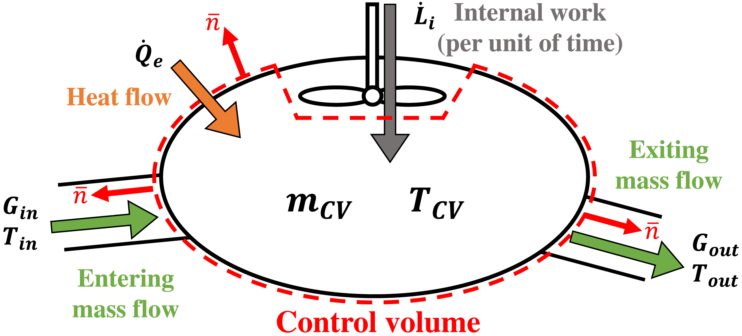
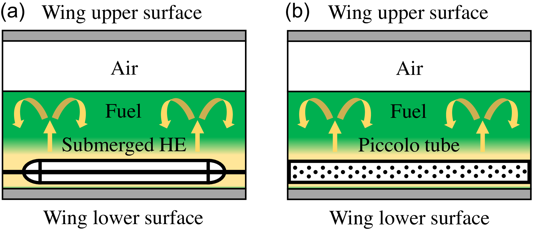


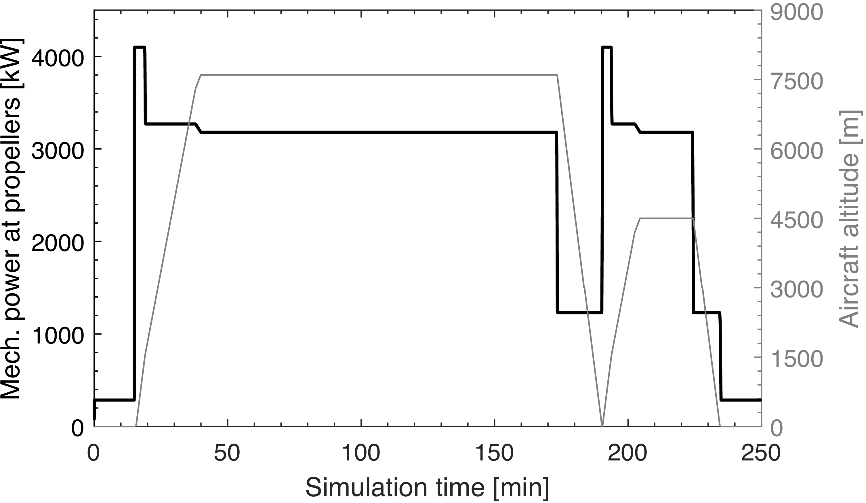


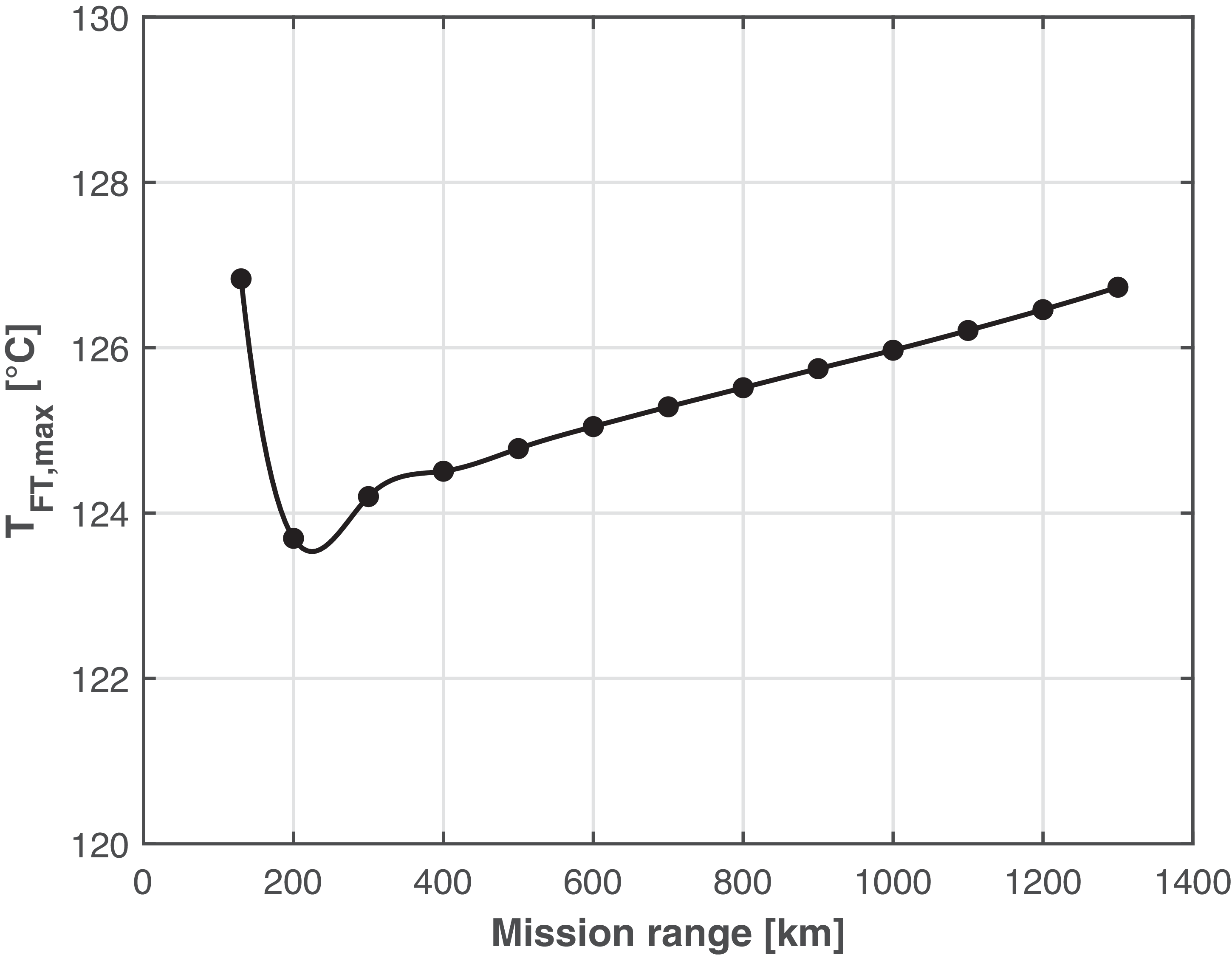

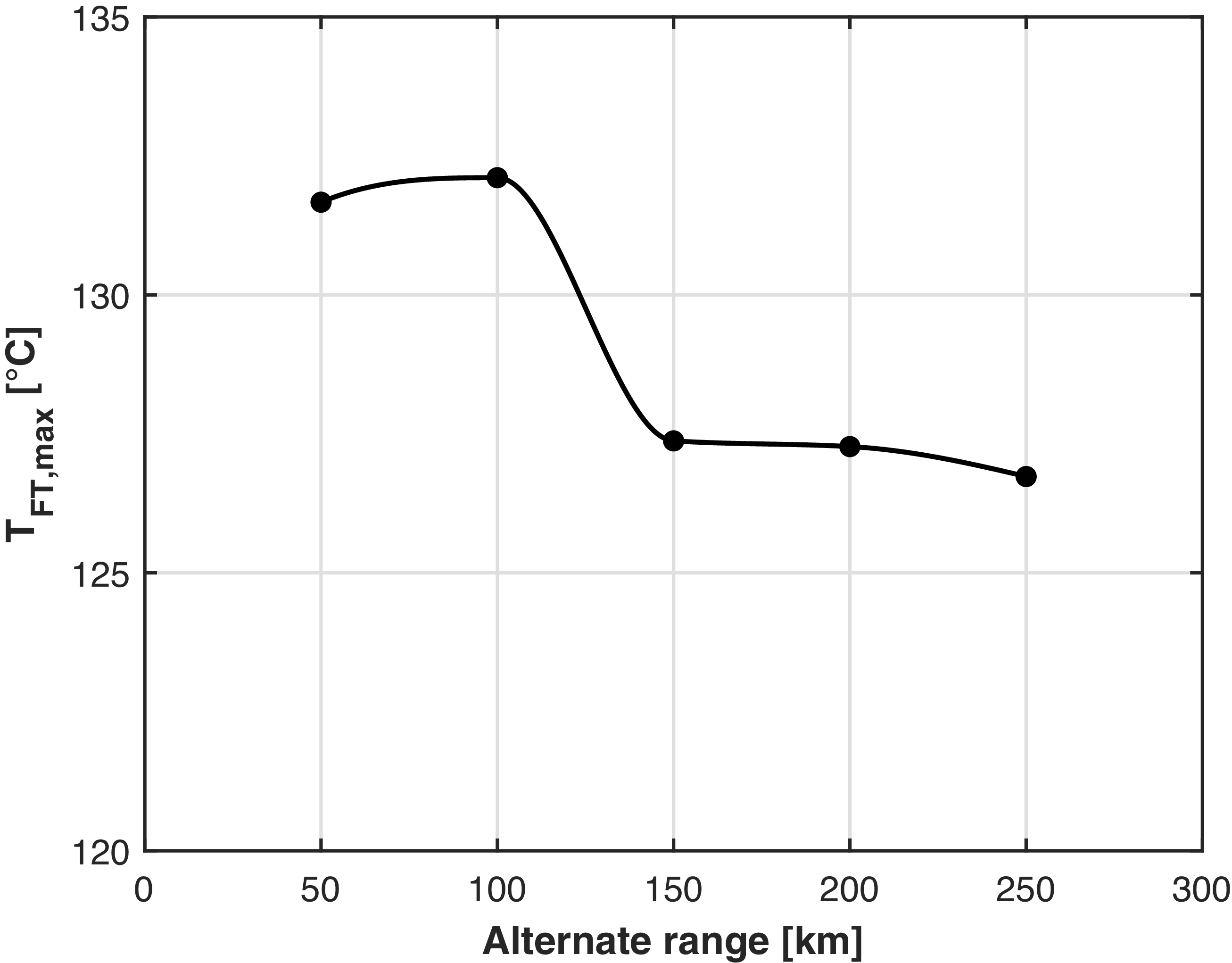


 ∘C


