1 Introduction
Wall pressure fluctuations induced by turbulent boundary layer (TBL) flows raise several engineering issues such as trailing edge noise, vibrations of structures which in turn generate acoustic radiations and disturbances for towed underwater sonar and sonar domes. In the case of military naval architecture, the prediction and reduction of noise generated by elongated vibrating structures is crucial. In order to analyse their stochastic response to wall pressure excitations, the space–time correlation function or the wavenumber–frequency spectrum is required.
Different regions can be defined for the pressure wavenumber–frequency spectrum: the supersonic region,
 $k<k_{a}$
, the subconvective region,
 $k_{a}<k<k_{c}$
, the convective region (or convective peak),
 $k\approx k_{c}$
, and the viscous region,
 $k\gg k_{c}$
(where
 $k_{a}=\unicode[STIX]{x1D714}/c$
is the acoustic wavenumber,
 $k_{c}=\unicode[STIX]{x1D714}/U_{c}$
is the convective wavenumber,
 $\unicode[STIX]{x1D714}$
is the radian frequency,
 $U_{c}$
is the convection velocity and
 $c$
is the sound velocity). The most energetic one is the convective region with pressure levels approximately 40 dB above the levels in the subconvective range (for an attached TBL with zero pressure gradient) (Bonness, Capone & Hambric Reference Bonness, Capone and Hambric2010). In the case of aircraft applications with high Mach number flows, significant vibrations are caused by pressure-field components with wavenumbers of the convective range which match the wavenumbers of the structure bending waves (Graham Reference Graham1997). However, for underwater applications, the convective peak may not be the only important part of the pressure spectrum. For low Mach number flows over elongated structures, strong structural responses result from excitation by pressure-field components with low wavenumbers which match those of the subconvective region (Bull Reference Bull1996; Bonness et al.
Reference Bonness, Capone and Hambric2010). Moreover, as the sound velocity is higher in water and the vehicle speeds are lower, the acoustic and convective wavenumbers are shifted downward and upward respectively. Thus, the subconvective range is larger for underwater applications.
Accurate predictions of the pressure spectrum may be obtained using direct numerical simulation (DNS) or large-eddy simulation (LES) (Choi & Moin Reference Choi and Moin1990; Chang, Piomelli & Blake Reference Chang, Piomelli and Blake1999; Hu, Morfey & Sandham Reference Hu, Morfey and Sandham2006; Wang et al. Reference Wang, Moreau, Iaccarino and Roger2009). However, the computation time for these simulations is still too large for complex industrial problems where numerous simulations have to be done. Thus, modelling techniques still have to be developed and used to predict the pressure loading.
Numerous semi-empirical models for the pressure spectrum can be found in the literature. They were proposed during the last decades for the frequency spectrum
 $\unicode[STIX]{x1D6F7}_{pp}(\unicode[STIX]{x1D714})$
and the wavenumber–frequency spectrum
 $\unicode[STIX]{x1D6F7}(k_{1},k_{3},\unicode[STIX]{x1D714})=\unicode[STIX]{x1D6F7}(\boldsymbol{k},\unicode[STIX]{x1D714})$
(where
 $k_{1}$
and
 $k_{3}$
are the streamwise and spanwise wavenumbers respectively,
 $\boldsymbol{k}=(k_{1},0,k_{3})$
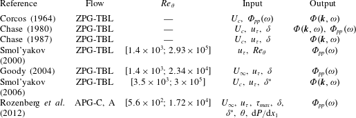
is the wave vector). Detailed reviews of frequently used models for the pressure spectrum can be found in the papers of Graham (Reference Graham1997) and Hwang, Bonness & Hambric (Reference Hwang, Bonness and Hambric2009). A few of them are presented in table 1. These models are based on data fitting and a certain degree of analytical and theoretical modelling. They only need few boundary layer characteristics as input so they are well adapted for design phases. However, they were mostly developed for zero pressure gradient turbulent boundary layers with ideal conditions, which may be far from the conditions of interest. Rozenberg, Robert & Moreau (Reference Rozenberg, Robert and Moreau2012) showed that empirical models for the frequency spectrum underestimate the spectral levels, particularly at low frequencies, in case of adverse pressure gradient (APG). Thus, they proposed a frequency spectrum model based on Goody (Reference Goody2004) which takes into account pressure gradient effects but it is restricted to APG. Moreover, for the wavenumber–frequency spectrum, the available semi-empirical models agree around the convective peak but show large discrepancies in the low wavenumber range which is also an area of interest.
Wall pressure spectra semi-empirical models. Flow: ZPG-TBL, zero pressure gradient turbulent boundary layer; C, channel; A, airfoil; APG, adverse pressure gradient.
 $Re_{\unicode[STIX]{x1D703}}=U_{\infty }\unicode[STIX]{x1D703}/\unicode[STIX]{x1D708}$
with:
 $U_{\infty }$
, free-stream velocity;
 $\unicode[STIX]{x1D708}$
, kinematic viscosity;
 $\unicode[STIX]{x1D703}$
, momentum thickness. Input:
 $U_{c}$
, convection velocity;
 $u_{\unicode[STIX]{x1D70F}}$
, friction velocity;
 $\unicode[STIX]{x1D6FF}$
, boundary layer thickness;
 $\unicode[STIX]{x1D6FF}^{\ast }$
, displacement thickness;
 $\unicode[STIX]{x1D70F}_{max}$
, maximum shearing stress along the normal;
 $\text{d}P/\text{d}x_{1}$
, mean pressure gradient. Output:
 $\unicode[STIX]{x1D6F7}_{pp}(\unicode[STIX]{x1D714})$
, wall pressure frequency spectrum;
 $\unicode[STIX]{x1D6F7}(\boldsymbol{k},\unicode[STIX]{x1D714})$
, wall pressure wavenumber–frequency spectrum.

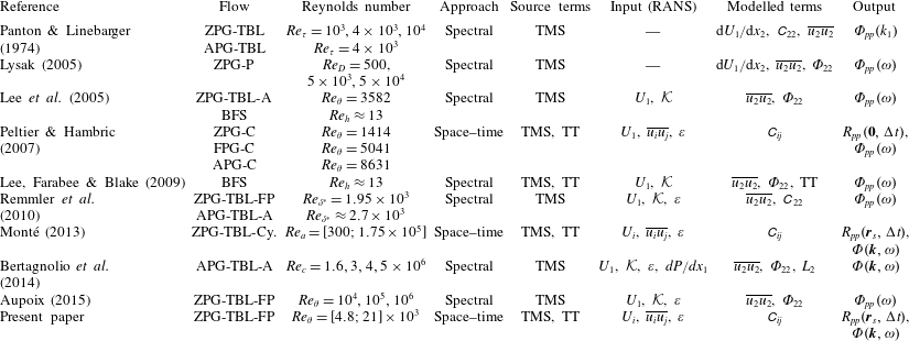
Another method is to express a solution to the Poisson equation for the pressure which relates wall pressure fluctuations to velocity sources in the turbulent flow. These source terms consist of the turbulence–mean shear (TMS) terms and the turbulence–turbulence (TT) terms, which are also referred to as rapid and slow terms respectively. Two kinds of approaches can be considered: a spectral solution which gives an expression for the wavenumber–frequency pressure spectrum; a space–time solution which gives an expression for the pressure fluctuation correlations. A few examples of both strategies are presented in table 2. The former approach was first applied by Kraichnan (Reference Kraichnan1956) who expressed the wavenumber–frequency spectrum for a TBL flow over a flat plate as a double integral over the wall-normal coordinate. His expression was obtained by taking into account only the linear TMS term and supposing the homogeneity of the TBL in planes parallel to the wall. This form involves the gradient of the mean streamwise velocity in the wall-normal direction and the Fourier transform of the vertical velocity correlations. The latter can be modelled using the Reynolds stress
 $\overline{u_{2}u_{2}}$
and the vertical velocity correlation coefficient
 $\unicode[STIX]{x1D60A}_{22}$
or a spectral correlation function
 $\unicode[STIX]{x1D6F7}_{22}$
. Based on the work of Kraichnan (Reference Kraichnan1956), several authors have proposed similar relationships for the pressure spectrum (see table 2). Panton & Linebarger (Reference Panton and Linebarger1974) used empirical models for the mean velocity and the velocity correlations as input for their expression. Blake (Reference Blake1986) used a derived expression for the frequency spectrum and deduced some characteristics for the spectrum due to the TMS term. Lysak (Reference Lysak2005) applied the method to turbulent pipe flows. In more recent works, Reynolds-averaged Navier–Stokes (RANS) solutions are used as input data for relationships similar to Kraichnan (Reference Kraichnan1956) which are applied to TBL flows without a pressure gradient (e.g. Aupoix Reference Aupoix2015) or to more complex flows such as flow over a backward-facing step (Lee, Blake & Farabee Reference Lee, Blake and Farabee2005) or over an airfoil (Remmler et al.
Reference Remmler, Christophe, Anthoine and Moreau2010; Bertagnolio, Fischer & Jun Zhu Reference Bertagnolio, Fischer and Jun Zhu2014).
Wall pressure spectra models solving the Poisson equation for the pressure fluctuations. Flow: ZPG, zero pressure gradient; FPG, favourable pressure gradient; APG, adverse pressure gradient; TBL, turbulent boundary layer; C, channel; P, pipe; BFS, backward-facing step; FP, over a flat plate; Cy., over a cylinder; A, over an airfoil. Reynolds number:
 $Re_{\unicode[STIX]{x1D70F}}=u_{\unicode[STIX]{x1D70F}}\unicode[STIX]{x1D6FF}/\unicode[STIX]{x1D708}$
;
 $Re_{\unicode[STIX]{x1D703}}=U_{\infty }\unicode[STIX]{x1D703}/\unicode[STIX]{x1D708}$
;
 $Re_{c}=U_{\infty }c/\unicode[STIX]{x1D708}$
,
 $Re_{D}=u_{\unicode[STIX]{x1D70F}}D/\unicode[STIX]{x1D708}$
and
 $Re_{a}=U_{\infty }a/\unicode[STIX]{x1D708}$
with:
 $u_{\unicode[STIX]{x1D70F}}$
, friction velocity;
 $U_{\infty }$
, free-stream velocity;
 $\unicode[STIX]{x1D6FF}$
, boundary layer thickness;
 $\unicode[STIX]{x1D703}$
, momentum thickness;
 $c$
, chord length;
 $D$
, pipe diameter;
 $a$
, cylinder radius;
 $\unicode[STIX]{x1D708}$
, kinematic viscosity. Input: input data from RANS solutions,
 $U_{1}$
, mean streamwise velocity;
 $\overline{u_{i}u_{j}}$
, Reynolds stresses;
 ${\mathcal{K}}$
, kinetic energy;
 $\unicode[STIX]{x1D700}$
, turbulent dissipation rate;
 $\text{d}P/\text{d}x_{1}$
, mean pressure gradient. Modelled terms:
 $\unicode[STIX]{x1D60A}_{ij}$
, space–time velocity correlation coefficients;
 $\unicode[STIX]{x1D6F7}_{22}$
, spectral correlation function associated with the vertical velocity fluctuations;
 $L_{2}$
, vertical correlation length. Output:
 $\unicode[STIX]{x1D6F7}_{pp}(\unicode[STIX]{x1D714})$
, wall pressure frequency spectrum;
 $\unicode[STIX]{x1D6F7}(\boldsymbol{k},\unicode[STIX]{x1D714})$
, wall pressure wavenumber–frequency spectrum;
 $R_{pp}$
, wall pressure correlations;
 $\boldsymbol{r}_{s}$
, space separation vector;
 $\unicode[STIX]{x0394}t$
, time separation.

As the Poisson equation for the wall pressure fluctuations with the nonlinear TT source terms cannot be solved directly in the spectral domain, these terms are disregarded in the Kraichnan (Reference Kraichnan1956) relation and similar works. Neglecting the TT source terms is often considered as a satisfactory assumption, particularly at mid and high frequencies (Kraichnan Reference Kraichnan1956; Panton & Linebarger Reference Panton and Linebarger1974; Remmler et al.
Reference Remmler, Christophe, Anthoine and Moreau2010). However, when the area of interest is located at low frequencies and wavenumbers, the TT source terms should not be neglected. Besides, Chang et al. (Reference Chang, Piomelli and Blake1999) showed, using DNS data for a fully developed turbulent channel flow at low Reynolds number, that the TMS and TT terms are of the same order throughout the wavenumber range. In order to take into account the TT terms, Lee et al. (Reference Lee, Farabee and Blake2009) tried to include heuristically a nonlinear source term, based on the DNS results of Kim (Reference Kim1989), in a spectral relation. They obtained satisfactory results for a flow over a backward-facing step. As an alternative, a more accurate and general way to estimate the TT terms contribution may be to solve the Poisson equation in the space–time domain. This approach is performed by Peltier & Hambric (Reference Peltier and Hambric2007) who proposed a stochastic model to estimate wall pressure spectra. A space–time solution to the Poisson equation for wall pressure correlations is used and the pressure spectrum is obtained by their Fourier transform. The TMS and TT source terms are expressed as a double integral over the space above the wall. The relation of Peltier & Hambric (Reference Peltier and Hambric2007) involves the gradient of the mean streamwise velocity in the wall-normal direction and four space–time velocity correlation functions. These latter are modelled as a product of velocity correlation coefficients (denoted by
 $\unicode[STIX]{x1D60A}_{ij}$
), which are obtained using a semi-empirical model developed by Gavin (Reference Gavin2002), and Reynolds stresses which are obtained by RANS solutions. Their model was able to correctly predict the effects of pressure gradients on wall pressure frequency spectra for a channel flow. Their results show that the TT contribution is smaller than the TMS one but not negligible. Monté (Reference Monté2013) applied a similar method to estimate the wavenumber–frequency spectrum for TBL flows over towed underwater antennas.
In the present work, we propose a new model to compute the pressure correlations, referred to as the Kriging-based elliptic extended anisotropic model (KEEAM), which relies on an expression similar to Peltier & Hambric (Reference Peltier and Hambric2007) for the pressure correlations and a new closure model for the velocity correlations based on the DNS results of Sillero, Jiménez & Moser (Reference Sillero, Jiménez and Moser2014). RANS data, obtained with Reynolds stress models, are also used as an input. The evaluation of wall pressure correlations is detailed in § 2 and the velocity correlation model is described in § 3. The present work focuses on the validation of the method and the velocity correlation model for a TBL flow over a flat plate. The results are presented in § 4 where they are discussed. Contrary to Peltier & Hambric (Reference Peltier and Hambric2007), both frequency and wavenumber–frequency spectra are computed. The influence of both the closure model and the Reynolds number on the pressure spectrum are investigated. The results are also compared to other approaches previously described.
2 Wall pressure correlations and spectrum
The instantaneous velocity components in the streamwise (
 $x_{1}$
), wall-normal (
 $x_{2}$
) and spanwise (
 $x_{3}$
) directions are denoted by
 $\tilde{u} _{1}$
,
 $\tilde{u} _{2}$
,
 $\tilde{u} _{3}$
, respectively. The instantaneous pressure is indicated by
 $\tilde{p}$
. Points on the wall are denoted by
 $\boldsymbol{x}_{s}$
and
 $\boldsymbol{y}_{s}$
. Points
 $\boldsymbol{x}$
and
 $\boldsymbol{y}$
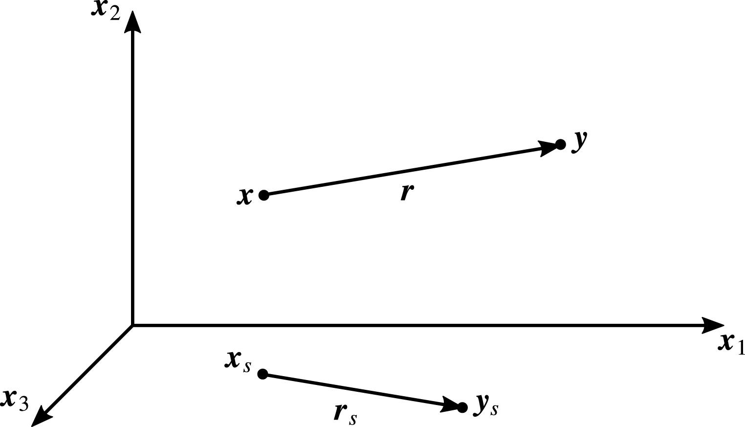
are located in the volume above the wall (see figure 1). Times are denoted by
 $t$
and
 $\unicode[STIX]{x1D70F}$
. An instantaneous variable
 $\tilde{a}$
is decomposed into mean part and fluctuation as:
 $\tilde{a}=A+a$
(Reynolds decomposition). Mean field quantities are represented in upper case and fluctuations in lower case.
Sketch of the spatial computational domain.

2.1 Equation for the wall pressure correlation
2.1.1 General formulation
The Poisson equation for the instantaneous pressure is obtained by taking the divergence of the incompressible Navier–Stokes equations. By integrating the resulting equation using an appropriate Green function
 $G$
and by neglecting the normal derivative of the pressure at the wall, a solution for the wall pressure can be written (Kraichnan Reference Kraichnan1956; Chassaing Reference Chassaing2000):
 $$\begin{eqnarray}\frac{1}{\unicode[STIX]{x1D70C}}\tilde{p}(\boldsymbol{x}_{s},t)=-\int _{\unicode[STIX]{x1D6FA}_{x}}\frac{\unicode[STIX]{x2202}}{\unicode[STIX]{x2202}x_{i}}\left(\tilde{u} _{j}(\boldsymbol{x},t)\frac{\unicode[STIX]{x2202}\tilde{u} _{i}(\boldsymbol{x},t)}{\unicode[STIX]{x2202}x_{j}}\right)G(\boldsymbol{x},\boldsymbol{x}_{s})\,\text{d}\boldsymbol{x},\end{eqnarray}$$
where
 $\unicode[STIX]{x1D70C}$
is the fluid density. This equation shows that the surface pressure is determined by contributions from all parts of the velocity field over the wall.
The expression of the wall pressure fluctuations is obtained by applying Reynolds decomposition to separate the mean and fluctuating wall pressures and then subtracting the mean pressure:
 $$\begin{eqnarray}\displaystyle \frac{1}{\unicode[STIX]{x1D70C}}p(\boldsymbol{x}_{s},t) & = & \displaystyle \int _{\unicode[STIX]{x1D6FA}_{x}}\left[2\left(\frac{\unicode[STIX]{x2202}U_{i}(\boldsymbol{x})}{\unicode[STIX]{x2202}x_{j}}u_{j}(\boldsymbol{x},t)\right)\frac{\unicode[STIX]{x2202}G(\boldsymbol{x},\boldsymbol{x}_{s})}{\unicode[STIX]{x2202}x_{i}}\right.\nonumber\\ \displaystyle & & \displaystyle \left.-\,(u_{i}(\boldsymbol{x},t)u_{j}(\boldsymbol{x},t)-\overline{u_{i}u_{j}}(\boldsymbol{x}))\frac{\unicode[STIX]{x2202}^{2}G(\boldsymbol{x},\boldsymbol{x}_{s})}{\unicode[STIX]{x2202}x_{i}\unicode[STIX]{x2202}x_{j}}\right]\,\text{d}\boldsymbol{x}.\end{eqnarray}$$
In (2.2), the spatial derivative were transferred to the Green function via applications of integration by parts and the divergence theorem (see Peltier & Hambric Reference Peltier and Hambric2007). The overbar indicates an ensemble average.
The space–time correlations of the wall pressure fluctuations are obtained from the ensemble average of the product of (2.2) evaluated at two different points and two different times (
 $\boldsymbol{x}_{s},t$
) and (
 $\boldsymbol{y}_{s},\unicode[STIX]{x1D70F}$
):
 $$\begin{eqnarray}\displaystyle \frac{1}{\unicode[STIX]{x1D70C}^{2}}\overline{p(\boldsymbol{x}_{s},t)p(\boldsymbol{y}_{s},\unicode[STIX]{x1D70F})} & = & \displaystyle \int _{\unicode[STIX]{x1D6FA}_{x}}\int _{\unicode[STIX]{x1D6FA}_{y}}\left[4\frac{\unicode[STIX]{x2202}U_{i}}{\unicode[STIX]{x2202}x_{j}}\frac{\unicode[STIX]{x2202}V_{k}}{\unicode[STIX]{x2202}y_{l}}\overline{u_{j}v_{l}}\frac{\unicode[STIX]{x2202}G(\boldsymbol{x},\boldsymbol{x}_{s})}{\unicode[STIX]{x2202}x_{i}}\frac{\unicode[STIX]{x2202}G(\boldsymbol{y},\boldsymbol{y}_{s})}{\unicode[STIX]{x2202}y_{k}}\right.\nonumber\\ \displaystyle & & \displaystyle -\,2\frac{\unicode[STIX]{x2202}U_{i}}{\unicode[STIX]{x2202}x_{j}}\overline{u_{j}v_{k}v_{l}}\frac{\unicode[STIX]{x2202}G(\boldsymbol{x},\boldsymbol{x}_{s})}{\unicode[STIX]{x2202}x_{i}}\frac{\unicode[STIX]{x2202}^{2}G(\boldsymbol{y},\boldsymbol{y}_{s})}{\unicode[STIX]{x2202}y_{k}\unicode[STIX]{x2202}y_{l}}\nonumber\\ \displaystyle & & \displaystyle -\,2\frac{\unicode[STIX]{x2202}V_{k}}{\unicode[STIX]{x2202}y_{l}}\overline{v_{l}u_{i}u_{j}}\frac{\unicode[STIX]{x2202}G(\boldsymbol{y},\boldsymbol{y}_{s})}{\unicode[STIX]{x2202}y_{k}}\frac{\unicode[STIX]{x2202}^{2}G(\boldsymbol{x},\boldsymbol{x}_{s})}{\unicode[STIX]{x2202}x_{i}\unicode[STIX]{x2202}x_{j}}\nonumber\\ \displaystyle & & \displaystyle \left.+\,(\overline{u_{i}u_{j}v_{k}v_{l}}-\overline{u_{i}u_{j}}~\overline{v_{k}v_{l}})\frac{\unicode[STIX]{x2202}^{2}G(\boldsymbol{x},\boldsymbol{x}_{s})}{\unicode[STIX]{x2202}x_{i}\unicode[STIX]{x2202}x_{j}}\frac{\unicode[STIX]{x2202}^{2}G(\boldsymbol{y},\boldsymbol{y}_{s})}{\unicode[STIX]{x2202}y_{k}\unicode[STIX]{x2202}y_{l}}\right]\,\text{d}\boldsymbol{y}\,\text{d}\boldsymbol{x},\end{eqnarray}$$
with
 $U_{i}(\boldsymbol{x})$
the mean velocity at point
 $\boldsymbol{x}$
;
 $V_{k}(\boldsymbol{y})$
the mean velocity at point
 $\boldsymbol{y}$
;
 $u_{j}(\boldsymbol{x},t)$
the fluctuating velocity at point
 $\boldsymbol{x}$
and time
 $t$
;
 $v_{l}(\boldsymbol{y},\unicode[STIX]{x1D70F})$
the fluctuating velocity at point
 $\boldsymbol{y}$
and time
 $\unicode[STIX]{x1D70F}$
.
Assuming that the joint distribution of the fluctuating velocities is normal, equation (2.3) can be simplified. Indeed, the third-order correlation tensor is zero and the fourth-order correlation tensor can be written as a function of the second-order correlation tensor:
 $$\begin{eqnarray}\overline{u_{i}u_{j}v_{k}v_{l}}=\overline{u_{i}u_{j}}~\overline{v_{k}v_{l}}+\overline{u_{i}v_{k}}~\overline{u_{j}v_{l}}+\overline{u_{i}v_{l}}~\overline{u_{j}v_{k}}.\end{eqnarray}$$
This hypothesis is not accurate for the velocity but it allowed Peltier & Hambric (Reference Peltier and Hambric2007) to obtain satisfactory results for wall pressure correlations.
As a remark, in the case of isotropic turbulence, only the fourth-order correlation tensor appears in the pressure correlation equation. This tensor is expressed as a function of the second-order correlation tensor as in the case of a normal distribution but nothing is assumed for the third-order tensor. This is referred to as the quasi-normality hypothesis (Millionschikov Reference Millionschikov1941), which is known to yield accurate results for the pressure evaluation (Batchelor Reference Batchelor1951; Lesieur, Ossia & Métais Reference Lesieur, Ossia and Métais1999; Meldi & Sagaut Reference Meldi and Sagaut2013).
Finally, with the normality hypothesis, the space–time correlations of the wall pressure fluctuations take the form:
 $$\begin{eqnarray}\displaystyle \frac{1}{\unicode[STIX]{x1D70C}^{2}}\overline{p(\boldsymbol{x}_{s},t)p(\boldsymbol{y}_{s},\unicode[STIX]{x1D70F})} & = & \displaystyle \int _{\unicode[STIX]{x1D6FA}_{x}}\int _{\unicode[STIX]{x1D6FA}_{y}}\left[4\frac{\unicode[STIX]{x2202}U_{i}}{\unicode[STIX]{x2202}x_{j}}\frac{\unicode[STIX]{x2202}V_{k}}{\unicode[STIX]{x2202}y_{l}}\overline{u_{j}v_{l}}\frac{\unicode[STIX]{x2202}G(\boldsymbol{x},\boldsymbol{x}_{s})}{\unicode[STIX]{x2202}x_{i}}\frac{\unicode[STIX]{x2202}G(\boldsymbol{y},\boldsymbol{y}_{s})}{\unicode[STIX]{x2202}y_{k}}\right.\nonumber\\ \displaystyle & & \displaystyle \left.+\,2~\overline{u_{i}v_{k}}~\overline{u_{j}v_{l}}\frac{\unicode[STIX]{x2202}^{2}G(\boldsymbol{x},\boldsymbol{x}_{s})}{\unicode[STIX]{x2202}x_{i}\unicode[STIX]{x2202}x_{j}}\frac{\unicode[STIX]{x2202}^{2}G(\boldsymbol{y},\boldsymbol{y}_{s})}{\unicode[STIX]{x2202}y_{k}\unicode[STIX]{x2202}y_{l}}\right]\,\text{d}\boldsymbol{y}\,\text{d}\boldsymbol{x}.\end{eqnarray}$$
Two types of terms can be identified in (2.5): the first group on the right-hand side denotes turbulence–mean shear (TMS) interactions source terms and the second group on the right-hand side represents turbulence–turbulence (TT) interactions source terms.
In order to estimate turbulent pressure correlations from (2.5), several quantities are required: a Green function, the mean velocity field at two different points and two-point and two-time velocity correlations
 $\overline{u_{i}(\boldsymbol{x},t)v_{k}(\boldsymbol{y},\unicode[STIX]{x1D70F})}$
. The velocity field can be obtained by RANS solutions but the two-point and two-time velocity correlations (or space–time velocity correlations) have to be modelled.
The two-point two-time velocity correlations,
 $\unicode[STIX]{x1D619}_{ik}(\boldsymbol{x},\boldsymbol{y},t,\unicode[STIX]{x1D70F})=\overline{u_{i}(\boldsymbol{x},t)v_{k}(\boldsymbol{y},\unicode[STIX]{x1D70F})}$
, can be written as a function of Reynolds stresses (i.e. one-point velocity correlations) and a space–time correlation coefficient:
 $$\begin{eqnarray}\unicode[STIX]{x1D619}_{ik}(\boldsymbol{x},\boldsymbol{y},t,\unicode[STIX]{x1D70F})=\sqrt{\overline{u_{i}u_{i}}(\boldsymbol{x})}\sqrt{\overline{v_{k}v_{k}}(\boldsymbol{y})}~\unicode[STIX]{x1D60A}_{ik}(\boldsymbol{x},\boldsymbol{y},t,\unicode[STIX]{x1D70F}).\end{eqnarray}$$
Reynolds stresses can be obtained from RANS solutions and a closure model is needed for the space–time correlation coefficients. This model is detailed in § 3.
2.1.2 Flow over a flat plate
We consider the case of a fully developed turbulent boundary layer over a flat rigid plate in a flow with zero pressure gradient at low Mach number. In this flow, the boundary layer thickness increases slowly in the streamwise direction and the velocity field can be considered homogeneous in the (
 $x_{1}$
,
 $x_{3}$
) plane (parallel to the wall) with a good approximation. Moreover, we assume that the flow is statistically two-dimensional so Reynolds stresses are reduced to four terms (Pope Reference Pope2000):
 $\overline{u_{1}u_{1}}$
,
 $\overline{u_{2}u_{2}}$
,
 $\overline{u_{3}u_{3}}$
and
 $\overline{u_{1}u_{2}}$
. Considering these hypotheses and substituting (2.6) in (2.5), the wall pressure correlations are expressed as:
 $$\begin{eqnarray}\displaystyle & & \displaystyle \frac{1}{\unicode[STIX]{x1D70C}^{2}}\overline{p(\boldsymbol{x}_{s},t)p(\boldsymbol{y}_{s},\unicode[STIX]{x1D70F})}=\int _{\unicode[STIX]{x1D6FA}_{x}}\int _{\unicode[STIX]{x1D6FA}_{y}}\left[4\frac{\unicode[STIX]{x2202}U_{1}}{\unicode[STIX]{x2202}x_{2}}\frac{\unicode[STIX]{x2202}V_{1}}{\unicode[STIX]{x2202}y_{2}}\sqrt{\overline{u_{2}u_{2}}}\sqrt{\overline{v_{2}v_{2}}}\unicode[STIX]{x1D60A}_{22}\frac{\unicode[STIX]{x2202}G(\boldsymbol{x},\boldsymbol{x}_{s})}{\unicode[STIX]{x2202}x_{1}}\frac{\unicode[STIX]{x2202}G(\boldsymbol{y},\boldsymbol{y}_{s})}{\unicode[STIX]{x2202}y_{1}}\right.\nonumber\\ \displaystyle & & \displaystyle \qquad \left.+\,2~\sqrt{\overline{u_{i}u_{i}}}\sqrt{\overline{v_{k}v_{k}}}\unicode[STIX]{x1D60A}_{ik}\sqrt{\overline{u_{j}u_{j}}}\sqrt{\overline{v_{l}v_{l}}}\unicode[STIX]{x1D60A}_{jl}\frac{\unicode[STIX]{x2202}^{2}G(\boldsymbol{x},\boldsymbol{x}_{s})}{\unicode[STIX]{x2202}x_{i}\unicode[STIX]{x2202}x_{j}}\frac{\unicode[STIX]{x2202}^{2}G(\boldsymbol{y},\boldsymbol{y}_{s})}{\unicode[STIX]{x2202}y_{k}\unicode[STIX]{x2202}y_{l}}\right]\,\text{d}\boldsymbol{y}\,\text{d}\boldsymbol{x}.\end{eqnarray}$$
Finally, the Green function for a flat plate is:
 $$\begin{eqnarray}G(\boldsymbol{x},\boldsymbol{x}_{s})=-\frac{1}{2\unicode[STIX]{x03C0}}\frac{1}{\Vert \boldsymbol{x}-\boldsymbol{x}_{s}\Vert }.\end{eqnarray}$$
The relation for pressure correlations (2.7) is slightly different from the one of Peltier & Hambric (Reference Peltier and Hambric2007) because their definition of the velocity correlation coefficients differs from (2.6). There is also a difference for the velocity gradients: Peltier & Hambric (Reference Peltier and Hambric2007) assume that
 $\unicode[STIX]{x2202}U_{1}/\unicode[STIX]{x2202}x_{2}\approx \unicode[STIX]{x2202}V_{1}/\unicode[STIX]{x2202}y_{2}$
so only
 $\unicode[STIX]{x2202}U_{1}/\unicode[STIX]{x2202}x_{2}$
appears in their equation.
2.2 Wall pressure spectrum
We assume that wall pressure correlations can be written as a function of the spatial separation
 $\boldsymbol{r}_{s}=\boldsymbol{y}_{s}-\boldsymbol{x}_{s}$
and the time separation
 $\unicode[STIX]{x0394}t=\unicode[STIX]{x1D70F}-t$
:
 $$\begin{eqnarray}\overline{p(\boldsymbol{x}_{s},t)p(\boldsymbol{y}_{s},\unicode[STIX]{x1D70F})}=R_{pp}(\boldsymbol{r}_{s},\unicode[STIX]{x0394}t).\end{eqnarray}$$
The wall pressure wavenumber–frequency spectrum is commonly obtained by the Fourier transform of the pressure fluctuation correlations:
 $$\begin{eqnarray}\unicode[STIX]{x1D6F7}(k_{1},k_{3},\unicode[STIX]{x1D714})=\frac{1}{(2\unicode[STIX]{x03C0})^{3}}\int _{-\infty }^{\infty }\int _{-\infty }^{\infty }\int _{-\infty }^{\infty }R_{pp}(r_{s1},r_{s3},\unicode[STIX]{x0394}t)\text{e}^{-\text{i}(k_{1}r_{s1}+k_{3}r_{s3}+\unicode[STIX]{x1D714}\unicode[STIX]{x0394}t)}\,\text{d}r_{s1}\,\text{d}r_{s3}\,\text{d}\unicode[STIX]{x0394}t.\end{eqnarray}$$
The frequency spectrum is related to the pressure correlations and the wavenumber–frequency spectrum by:
 $$\begin{eqnarray}\unicode[STIX]{x1D6F7}_{pp}(\unicode[STIX]{x1D714})=\frac{1}{2\unicode[STIX]{x03C0}}\int _{-\infty }^{\infty }R_{pp}(0,0,\unicode[STIX]{x0394}t)\text{e}^{-\text{i}\unicode[STIX]{x1D714}\unicode[STIX]{x0394}t}\,\text{d}\unicode[STIX]{x0394}t=\int _{-\infty }^{\infty }\int _{-\infty }^{\infty }\unicode[STIX]{x1D6F7}(k_{1},k_{3},\unicode[STIX]{x1D714})\,\text{d}k_{1}\,\text{d}k_{3}.\end{eqnarray}$$
2.3 Numerical method
To evaluate (2.5) or (2.7), a double volume integral must be estimated numerically. Moreover, in the case of a flow over a flat plate, the Green function and its derivatives are singular for
 $\boldsymbol{x}=\boldsymbol{x}_{s}$
and
 $\boldsymbol{y}=\boldsymbol{y}_{s}$
. Since the velocity and the Reynolds stresses are zero on the wall, numerical problems occur only when
 $\boldsymbol{x}$
and
 $\boldsymbol{y}$
are close to
 $\boldsymbol{x}_{s}$
and
 $\boldsymbol{y}_{s}$
but above the wall. In this case, the integrand varies strongly. To take these variations into account, we use an adaptive quad-tree grid. This grid generation is based on an error estimator of the integration of the Green function derivatives. Integrations on each subspace of the grid are realized with a seventh-order discrete Gauss–Legendre method. The size of the integration domain is taken sufficiently large to guarantee the convergence of the results.
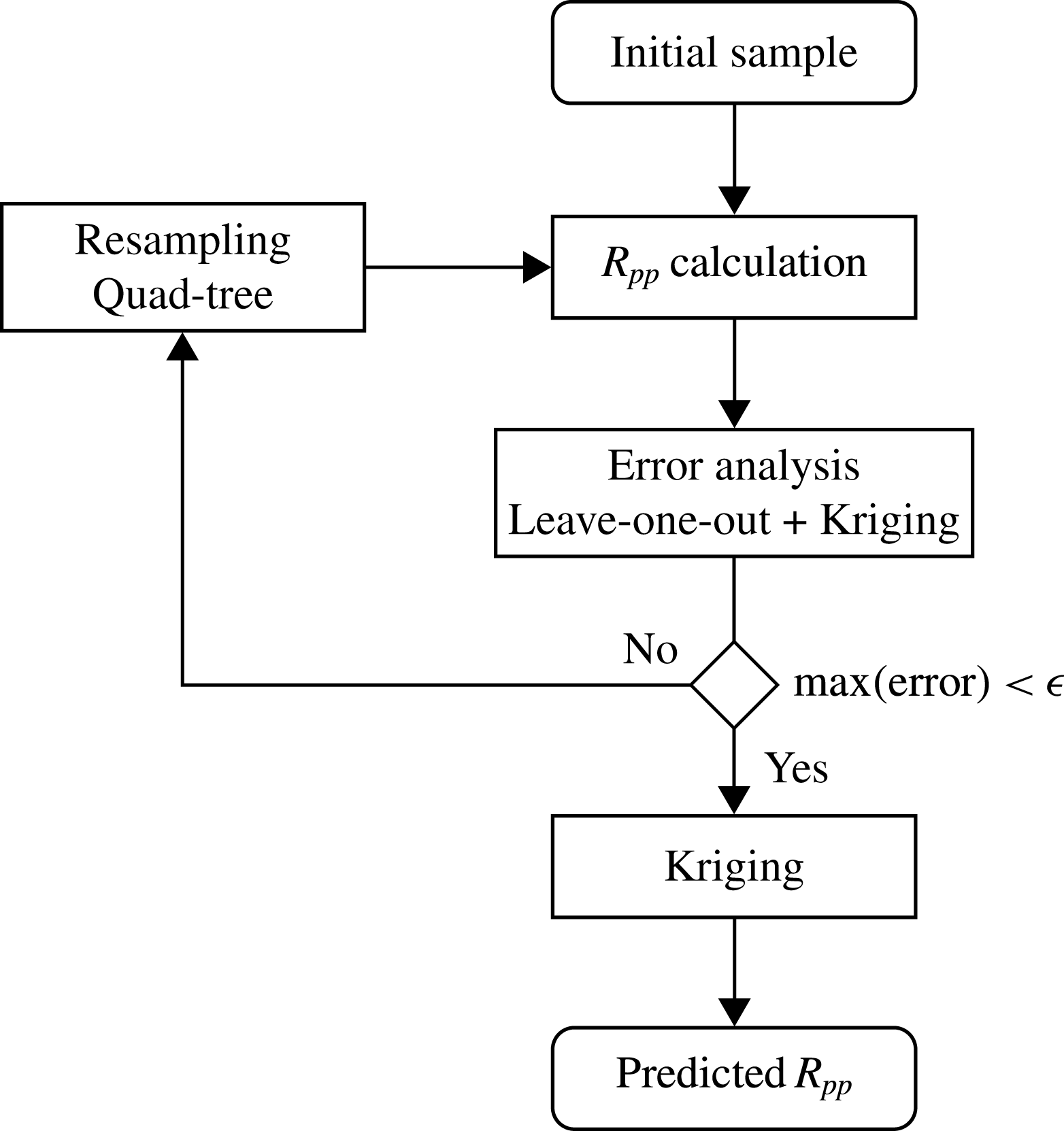
Besides, to obtain the pressure spectrum for broad frequency and wavenumber ranges, a considerable number of pressure correlation values are required. In order to reduce the computation time, we evaluate the pressure correlations only at a few points and create a surrogate model using Kriging (Krige Reference Krige1951). A self-adaptive sampling strategy is used to increase the accuracy of the surrogate model (see Braconnier et al.
Reference Braconnier, Ferrier, Jouhaud, Montagnac and Sagaut2011; Margheri & Sagaut Reference Margheri and Sagaut2016). Figure 2 shows the steps of the method. Starting from an initial sample with a uniform distribution, the pressure correlations are calculated. Then, using the leave-one-out cross-validation process, a local error is estimated for each point. Precisely, the sample is split into a training set (used to build the surrogate model with Kriging) and a test set (with only one point). The local error is evaluated between the pressure correlation value at the test point,
 $R_{pp}(X_{test})$
, and the value obtained with the surrogate model at the test point,
 $R_{pp}^{s}(X_{test})$
:
 $$\begin{eqnarray}LE=\frac{|R_{pp}(X_{test})-R_{pp}^{s}(X_{test})|}{R_{pp}(0,0,0)}.\end{eqnarray}$$
 $R_{pp}(0,0,0)$
is the maximal value of the pressure correlations and is computed in the initial sample. This error is estimated for each element of the sample and points are added with quad-tree sampling where the error is maximal. The pressure correlations are evaluated for the new points and the previous steps are repeated until a satisfactory error is reached. A minimal value is imposed for the distance between points in order to avoid accumulations near discontinuities or high gradients. Finally, the surrogate model is used to interpolate the pressure correlations on a fine grid.
For two-dimensional results with a local error lower than
 $5\,\%$
, approximately
 $500$
values of pressure correlations are required to compute a streamwise wavenumber–frequency spectrum on a
 $2048\times 2048$
grid. An example of the pressure frequency spectrum obtained with and without Kriging is presented in § 4.
Flowchart of the adaptive sampling method.

3 Two-point two-time velocity correlation model
3.1 Velocity correlation characteristics
Space and time dependencies are here systematically specified so the fluctuating velocity at point
 $\boldsymbol{y}$
and time
 $\unicode[STIX]{x1D70F}$
is also denoted
 $u_{i}$
without any confusion. Since the turbulent boundary layer is considered as stationary in time, the space–time velocity correlations can be written:
 $$\begin{eqnarray}\unicode[STIX]{x1D619}_{ij}(\boldsymbol{x},\boldsymbol{y},t,\unicode[STIX]{x1D70F})=\unicode[STIX]{x1D619}_{ij}(\boldsymbol{x},\boldsymbol{r},\unicode[STIX]{x0394}t)=\overline{u_{i}(\boldsymbol{x},t)u_{j}(\boldsymbol{x}+\boldsymbol{r},t+\unicode[STIX]{x0394}t)},\end{eqnarray}$$
with
 $\boldsymbol{r}=\boldsymbol{y}-\boldsymbol{x}$
the spatial separation vector and
 $\unicode[STIX]{x0394}t=\unicode[STIX]{x1D70F}-t$
the time separation.
Some conditions can be written for the form of the velocity correlations, which in turn, have an impact on the form of the correlation coefficients
 $\unicode[STIX]{x1D60A}_{ij}$
. It is assumed that the motion at one point of the fluid and one time is statistically independent of the motion at a point sufficiently distant in space or time. Thus,
 $\unicode[STIX]{x1D619}_{ij}$
should become negligible for large values of
 $|\boldsymbol{r}|$
or
 $\unicode[STIX]{x0394}t$
.
 $\unicode[STIX]{x1D619}_{ij}$
also vanishes when a point is located on the wall (i.e. when
 $x_{2}=0$
or
 $r_{2}=-x_{2}$
). The former requirement applies directly to
 $\unicode[STIX]{x1D60A}_{ij}$
and the last one is automatically satisfied using (2.6).
The form of the velocity correlations should also satisfy the continuity condition (Rotta Reference Rotta1962):
 $$\begin{eqnarray}\frac{\unicode[STIX]{x2202}}{\unicode[STIX]{x2202}r_{j}}\unicode[STIX]{x1D619}_{ij}(\boldsymbol{x},\boldsymbol{r},\unicode[STIX]{x0394}t)=0.\end{eqnarray}$$
Since the instantaneous flux across any closed surface is zero and
 $\unicode[STIX]{x1D619}_{ij}$
tends to zero at large
 $|\boldsymbol{r}|$
, the integration of (3.2) with respect to all values of
 $r_{2}$
and
 $r_{3}$
for a constant value of
 $r_{1}$
leads to (Rotta Reference Rotta1962; Townsend Reference Townsend1980):
 $$\begin{eqnarray}\int _{-\infty }^{\infty }\int _{-x_{2}}^{\infty }\unicode[STIX]{x1D619}_{i1}(\boldsymbol{x},\boldsymbol{r},\unicode[STIX]{x0394}t)\,\text{d}r_{2}\,\text{d}r_{3}=0,\quad i=1,2,3.\end{eqnarray}$$
Equation (3.3) implies that
 $\unicode[STIX]{x1D619}_{i1}$
has positive and negative values within the plane (
 $r_{2},r_{3}$
). Similar equations can be written for the other velocity correlations by integrating over planes (
 $r_{1},r_{3}$
) and (
 $r_{1}$
,
 $r_{2}$
). The condition (3.3) does not apply exactly to
 $\unicode[STIX]{x1D60A}_{ij}$
even if the coexistence of negative and positive regions can be observed (Sillero et al.
Reference Sillero, Jiménez and Moser2014).
Finally,
 $\unicode[STIX]{x1D619}_{ij}$
should tend to one-point correlations for
 $\boldsymbol{r}=\mathbf{0}$
and
 $\unicode[STIX]{x0394}t=0$
:
 $$\begin{eqnarray}\unicode[STIX]{x1D619}_{ij}(\boldsymbol{x},\mathbf{0},0)=\overline{u_{i}u_{j}}(\boldsymbol{x}),\end{eqnarray}$$
which implies for the correlation coefficient
 $\unicode[STIX]{x1D60A}_{ij}$
that:
 $$\begin{eqnarray}\displaystyle & \displaystyle \unicode[STIX]{x1D60A}_{ii}(\boldsymbol{x},\mathbf{0},0)=1 & \displaystyle\end{eqnarray}$$
 $$\begin{eqnarray}\displaystyle & \displaystyle \unicode[STIX]{x1D60A}_{ij}(\boldsymbol{x},\mathbf{0},0)=\frac{\overline{u_{i}u_{j}}(\boldsymbol{x})}{\sqrt{\overline{u_{i}u_{i}}(\boldsymbol{x})}\sqrt{\overline{u_{j}u_{j}}(\boldsymbol{x})}},\quad i\neq j. & \displaystyle\end{eqnarray}$$
For the sake of simplicity, we introduce
 $\tilde{\unicode[STIX]{x1D60A}}_{12}$
such as:
 $$\begin{eqnarray}\tilde{\unicode[STIX]{x1D60A}}_{12}(\boldsymbol{x},\boldsymbol{r},\unicode[STIX]{x0394}t)=\frac{\unicode[STIX]{x1D60A}_{12}(\boldsymbol{x},\boldsymbol{r},\unicode[STIX]{x0394}t)}{\unicode[STIX]{x1D60A}_{12}(\boldsymbol{x},\mathbf{0},0)},\end{eqnarray}$$
which satisfies
 $\tilde{\unicode[STIX]{x1D60A}}_{12}(\boldsymbol{x},\mathbf{0},0)=1$
.
The previous requirements help to define a form for the velocity correlation coefficients. To model these space–time coefficients we proceed in two steps:
3.2 Space correlation model
To model the spatial evolution of the velocity correlation coefficients we proposed a semi-analytical model (for
 $\unicode[STIX]{x1D60A}_{ii}$
and
 $\tilde{\unicode[STIX]{x1D60A}}_{12}$
) using the DNS data of Sillero et al. (Reference Sillero, Jiménez and Moser2014) as reference. The spatial characteristics of these data are detailed in § 3.2.1. The main characteristics of the isotropic model and the simplified anisotropic model (SAM) are given in §§ 3.2.2 and 3.2.3 respectively. Both approaches are used as a basis for the new
 $\unicode[STIX]{x1D60A}_{ij}$
form, referred to as extended anisotropic model (EAM), proposed in this work and presented in § 3.2.4. Lastly, these three models are compared in § 3.2.5.
3.2.1 Spatial characteristics from reference data
Sillero et al. (Reference Sillero, Jiménez and Moser2014) give detailed results of two-point statistics, particularly velocity correlation coefficients, for the buffer, logarithmic and outer regions of turbulent boundary layers. Data are available for three Reynolds number
 $Re_{\unicode[STIX]{x1D703}}\approx 4000,4860\text{ and }6500$
(where
 $Re_{\unicode[STIX]{x1D703}}=U_{\infty }\unicode[STIX]{x1D703}/\unicode[STIX]{x1D708}$
,
 $U_{\infty }$
is the free-stream velocity,
 $\unicode[STIX]{x1D708}$
is the kinematic viscosity and
 $\unicode[STIX]{x1D703}$
is the momentum thickness). These data can be found athttp://torroja.dmt.upm.es/turbdata/blayers/high_re/correlations.
Streamwise (
 $r_{1}$
,
 $r_{2}$
) sections of the correlation coefficients obtained with the DNS data of Sillero et al. (Reference Sillero, Jiménez and Moser2014) for
 $r_{3}=0$
,
 $\unicode[STIX]{x0394}t=0$
,
 $x_{2}/\unicode[STIX]{x1D6FF}=0.065$
and
 $Re_{\unicode[STIX]{x1D703}}\approx 4860$
(the flow is from left to right). Positive contours (——) are from
 $0.1$
to
 $0.9$
with increments of
 $0.1$
, the negative contours (- - -) are
 $[-0.1;-0.05]$
.

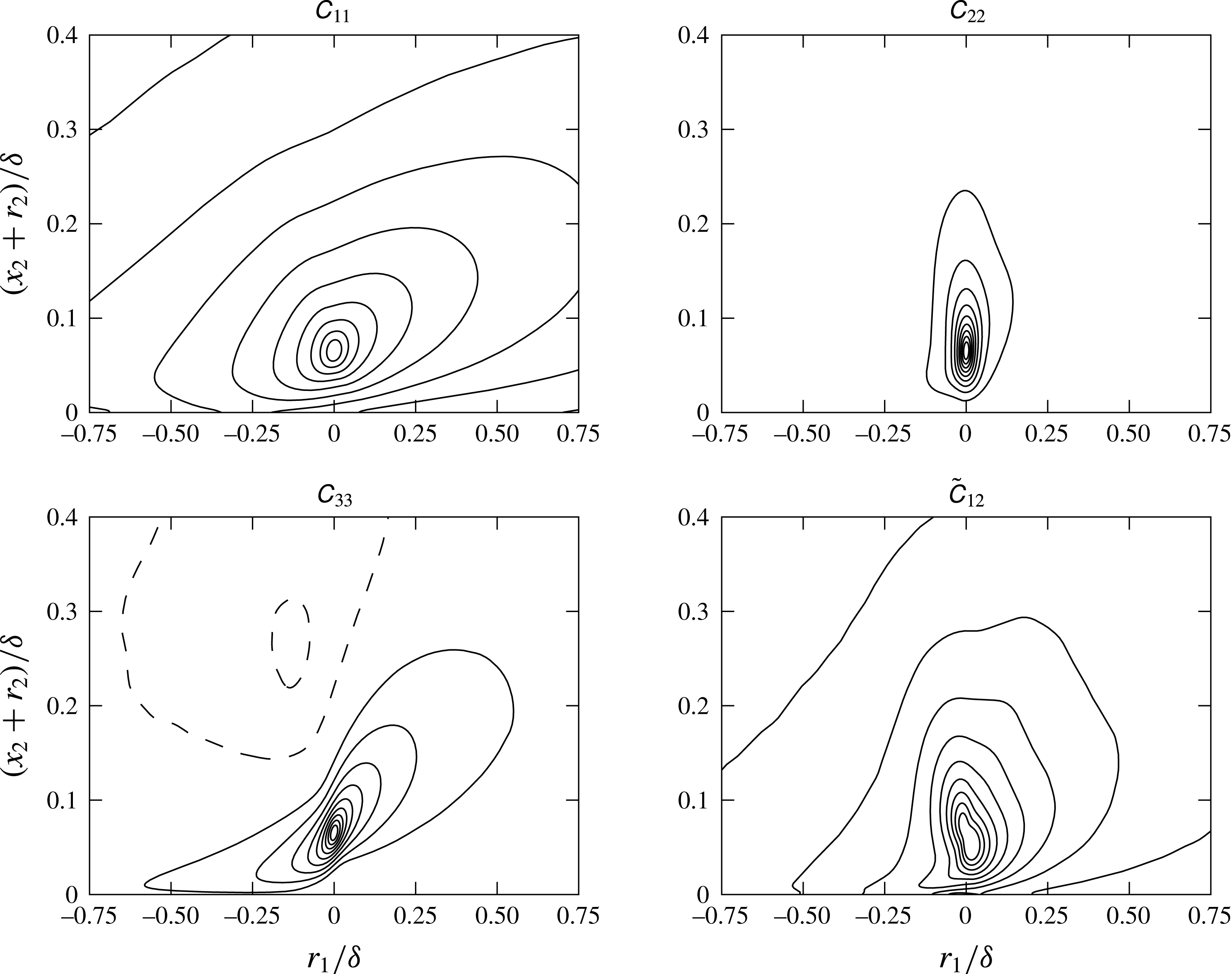
An example of sections of the four correlation coefficients in the plane (
 $r_{1}$
,
 $r_{2}$
), obtained by post-processing the Sillero et al. (Reference Sillero, Jiménez and Moser2014) data, are presented in figure 3. The variables are scaled by the boundary layer thickness
 $\unicode[STIX]{x1D6FF}$
. Correlation coefficients are more or less elongated structures tilted with respect to the wall. Sillero et al. (Reference Sillero, Jiménez and Moser2014) observed that their size in the three directions as well as their inclination angle depend on the variable being considered and the wall distance
 $x_{2}$
. The streamwise velocity correlation coefficient
 $\unicode[STIX]{x1D60A}_{11}$
is more elongated than the others in the streamwise direction (see figure 3). Its maximum length observed for the weakly correlated structures (
 $\unicode[STIX]{x1D60A}_{11}\approx 0.025$
) is of the order of
 $7\unicode[STIX]{x1D6FF}$
(see also the experimental results of Tutkun et al. (Reference Tutkun, George, Delville, Stanislas, Johansson, Foucaut and Coudert2009)) whereas for
 $\unicode[STIX]{x1D60A}_{22}$
and
 $\unicode[STIX]{x1D60A}_{33}$
the maximum streamwise length is of the order of
 $2\unicode[STIX]{x1D6FF}$
–
 $\unicode[STIX]{x1D6FF}$
. On the contrary, these three coefficients have similar spanwise widths of the order of
 $\unicode[STIX]{x1D6FF}$
. However, the size of these coefficients in each direction evolve differently with the wall distance
 $x_{2}$
. The value of the inclination angle depends on the correlation level being considered (see figure 3) but Sillero et al. (Reference Sillero, Jiménez and Moser2014) define a characteristic inclination angle which is the maximum angle observed as a function of the wall distance
 $x_{2}$
. For
 $\unicode[STIX]{x1D60A}_{11}$
, the angle is
 $\unicode[STIX]{x1D6FC}_{1}\approx 10^{\circ }$
. For
 $\unicode[STIX]{x1D60A}_{33}$
, the inclination angle tends quickly to a steeper one,
 $\unicode[STIX]{x1D6FC}_{3}\approx 32^{\circ }$
. Both angles are principally uniform across the boundary height.
 $\unicode[STIX]{x1D60A}_{22}$
is mainly vertical except in a region close to the wall where
 $\unicode[STIX]{x1D6FC}_{2}\approx \unicode[STIX]{x1D6FC}_{1}$
. Finally,
 $\tilde{\unicode[STIX]{x1D60A}}_{12}$
looks like a shorter version of
 $\unicode[STIX]{x1D60A}_{11}$
(Sillero et al.
Reference Sillero, Jiménez and Moser2014).
3.2.2 Isotropic model
In the case of isotropic turbulence, the velocity correlations can be expressed as (Batchelor Reference Batchelor1959; Sagaut & Cambon Reference Sagaut and Cambon2008):
 $$\begin{eqnarray}\unicode[STIX]{x1D619}_{ij}(\boldsymbol{r})=\overline{u_{i}(\boldsymbol{x})u_{j}(\boldsymbol{x}+\boldsymbol{r})}=u^{2}\left(\frac{f(r)-g(r)}{r^{2}}r_{i}r_{j}+g(r)\unicode[STIX]{x1D6FF}_{ij}\right),\end{eqnarray}$$
where
 $u^{2}=2{\mathcal{K}}/3$
is a scaling factor function of the kinetic energy
 ${\mathcal{K}}$
;
 $\unicode[STIX]{x1D6FF}_{ij}$
is the Kronecker delta;
 $f$
and
 $g$
are the longitudinal and transverse correlation functions respectively,
 $r$
is the norm of the spatial separation vector
 $\boldsymbol{r}$
.
The correlation function
 $g$
is linked to
 $f$
via the continuity condition (3.2) which leads to:
 $$\begin{eqnarray}g(r)=f(r)+\frac{r}{2}\frac{\unicode[STIX]{x2202}f(r)}{\unicode[STIX]{x2202}r}.\end{eqnarray}$$
These functions have to satisfy
 $f(0)=g(0)=1$
. A common expression for the correlation function
 $f$
is (Panton & Linebarger Reference Panton and Linebarger1974; Peltier & Hambric Reference Peltier and Hambric2007):
 $$\begin{eqnarray}f(r)=\exp \left(-\frac{r}{L}\right),\end{eqnarray}$$
where
 $L$
is a correlation length. Different formulas can be used for
 $L$
such as Taylor microscale
 $\unicode[STIX]{x1D706}_{f}=\sqrt{15\unicode[STIX]{x1D708}u^{2}/\unicode[STIX]{x1D700}}$
or a characteristic integral scale
 $L_{u}={\mathcal{K}}^{3/2}/\unicode[STIX]{x1D700}$
(Sagaut & Cambon Reference Sagaut and Cambon2008) which are both functions of the kinetic energy dissipation rate
 $\unicode[STIX]{x1D700}$
. With (3.10), the condition that
 $\unicode[STIX]{x1D619}_{ij}$
should vanish for large values of
 $|\boldsymbol{r}|$
is satisfied.
From (3.8), the correlation coefficients can be written:
 $$\begin{eqnarray}\displaystyle & \displaystyle \unicode[STIX]{x1D60A}_{ii}(\boldsymbol{r})=\frac{f(r)-g(r)}{r^{2}}r_{i}r_{i}+g(r) & \displaystyle\end{eqnarray}$$
 $$\begin{eqnarray}\displaystyle & \displaystyle \tilde{\unicode[STIX]{x1D60A}}_{12}(\boldsymbol{r})=\frac{f(r)-g(r)}{r^{2}}r_{1}r_{2}. & \displaystyle\end{eqnarray}$$
Streamwise (
 $r_{1}$
,
 $r_{2}$
) sections of the correlation coefficients obtained with the isotropic model (
 $L=0.54L_{u}$
) for
 $r_{3}=0$
,
 $\unicode[STIX]{x0394}t=0$
,
 $x_{2}/\unicode[STIX]{x1D6FF}=0.065$
and
 $Re_{\unicode[STIX]{x1D703}}\approx 4860$
(the flow is from left to right). For
 $\unicode[STIX]{x1D60A}_{11}$
,
 $\unicode[STIX]{x1D60A}_{22}$
and
 $\unicode[STIX]{x1D60A}_{33}$
, positive contours (——) are from
 $0.1$
to
 $0.9$
with increments of
 $0.1$
. For
 $\tilde{\unicode[STIX]{x1D60A}}_{12}$
, the positive contour (——) is 0.05 and the negative one (- - -) is
 $-0.05$
. The grey dotted contours are the DNS results of Sillero et al. (Reference Sillero, Jiménez and Moser2014) at the same height and Reynolds number.

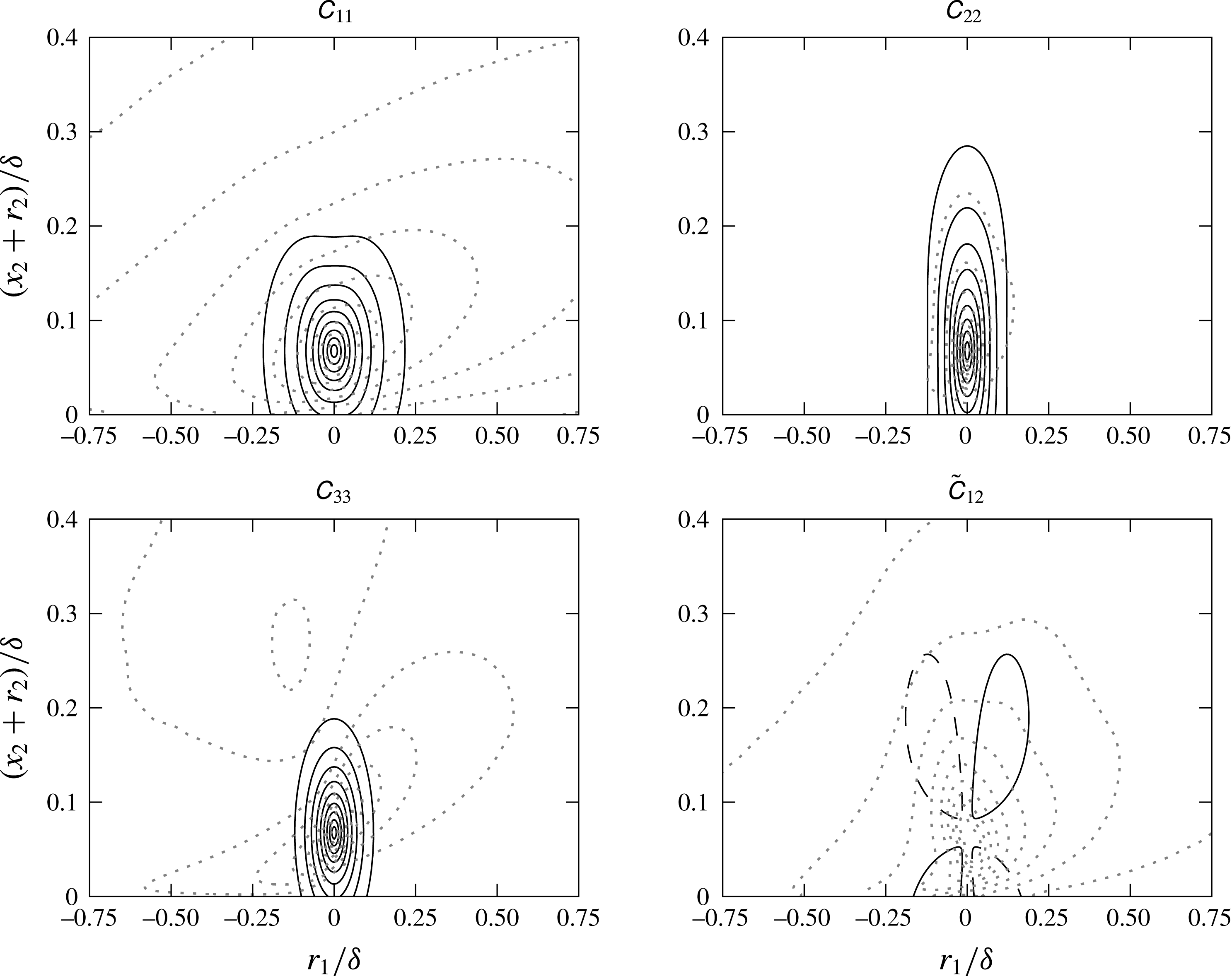
The four correlation coefficients obtained with the isotropic model are shown in the plane (
 $r_{1}$
,
 $r_{2}$
) in figure 4. The DNS results presented in figure 3 are also plotted (grey dotted lines) as a reference. The correlation length used for this figure is proportional to
 $L_{u}$
. It shows the necessity to take into account the inclination angles as well as the anisotropy effects. Indeed, only one correlation length for all the
 $\unicode[STIX]{x1D60A}_{ij}$
is not sufficient. Besides, the form of the model for
 $\tilde{\unicode[STIX]{x1D60A}}_{12}$
is clearly not adapted.
3.2.3 Simplified anisotropic model
The simplified anisotropic model, presented in Peltier & Hambric (Reference Peltier and Hambric2007), was developed by Gavin (Reference Gavin2002). It is an empirical model based on measurements of turbulent velocity correlations in the outer region of a high Reynolds number boundary layer. In order to take into account the ellipsoidal shape and the inclination of the velocity correlations to the wall, Gavin (Reference Gavin2002) defined a rotation angle
 $\unicode[STIX]{x1D703}$
and stretching coefficients
 $\unicode[STIX]{x1D6FE}_{i}$
to modify the separation vector
 $\boldsymbol{r}=\boldsymbol{y}-\boldsymbol{x}$
and then used a form similar to the isotropic model (3.8).
Firstly, a rotation is applied to the separation vector:
 $$\begin{eqnarray}\unicode[STIX]{x1D743}=\left[\begin{array}{@{}ccc@{}}\cos (\unicode[STIX]{x1D703}) & \sin (\unicode[STIX]{x1D703}) & 0\\ -\!\sin (\unicode[STIX]{x1D703}) & \cos (\unicode[STIX]{x1D703}) & 0\\ 0 & 0 & 1\end{array}\right]\left[\begin{array}{@{}c@{}}r_{1}\\ r_{2}\\ r_{3}\end{array}\right].\end{eqnarray}$$
Then, a separation length is defined using the stretching coefficients:
 $$\begin{eqnarray}r^{\ast }=\sqrt{\left(\frac{\unicode[STIX]{x1D709}_{1}}{\unicode[STIX]{x1D6FE}_{1}}\right)^{2}+\left(\frac{\unicode[STIX]{x1D709}_{2}}{\unicode[STIX]{x1D6FE}_{2}}\right)^{2}+\left(\frac{\unicode[STIX]{x1D709}_{3}}{\unicode[STIX]{x1D6FE}_{3}}\right)^{2}}.\end{eqnarray}$$
Finally, velocity correlation coefficients are written by adapting the model for the isotropic turbulence:
 $$\begin{eqnarray}\unicode[STIX]{x1D60A}_{ij}(\unicode[STIX]{x1D743})=\frac{\unicode[STIX]{x1D709}_{i}\unicode[STIX]{x1D709}_{j}}{{r^{\ast }}^{2}}[f(r^{\ast })-g(r^{\ast })]+\unicode[STIX]{x1D6FF}_{ij}g(r^{\ast }),\end{eqnarray}$$
with
 $f(r^{\ast })=\exp (-r^{\ast }/L)$
. The transverse correlation function
 $g$
is obtained using (3.9).
According to Peltier & Hambric (Reference Peltier and Hambric2007), Gavin used
 $L=0.35\unicode[STIX]{x1D6FF}$
for the correlation length which is valid only in the outer region of the TBL. Instead, they use
 $L(x_{2})\equiv 0.54L_{u}(x_{2})$
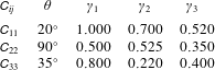
. The values of the SAM parameters determined by Gavin are presented in table 3. Since no values are given for
 $\tilde{\unicode[STIX]{x1D60A}}_{12}$
, we use
 $\tilde{\unicode[STIX]{x1D60A}}_{12}\approx \sqrt{|\unicode[STIX]{x1D60A}_{11}\unicode[STIX]{x1D60A}_{22}|}$
as Peltier & Hambric (Reference Peltier and Hambric2007).
SAM parameters.

Streamwise (
 $r_{1}$
,
 $r_{2}$
) sections of the correlation coefficients obtained with the SAM (
 $L=0.54L_{u}$
) for
 $r_{3}=0$
,
 $\unicode[STIX]{x0394}t=0$
,
 $x_{2}/\unicode[STIX]{x1D6FF}=0.065$
and
 $Re_{\unicode[STIX]{x1D703}}\approx 4860$
(the flow is from left to right). Positive contours (——) are from
 $0.1$
to
 $0.9$
with increments of
 $0.1$
. The grey dotted contours are the DNS results of Sillero et al. (Reference Sillero, Jiménez and Moser2014) at the same height and Reynolds number.

The resulting correlation coefficients are plotted in figure 5 and compared with the DNS results of Sillero et al. (Reference Sillero, Jiménez and Moser2014). The SAM angles appear to be too large, particularly for
 $\unicode[STIX]{x1D60A}_{11}$
. However, it depends on the correlation level being considered. Except
 $\unicode[STIX]{x1D60A}_{22}$
, the
 $\unicode[STIX]{x1D60A}_{ij}$
coefficients decay too fast which implies that the correlation length is too small for this value of
 $x_{2}$
. Other drawbacks of the SAM are that the lengths of the coefficients in each direction evolve similarly as functions of
 $x_{2}$
which is not expected (see Sillero et al.
Reference Sillero, Jiménez and Moser2014). Moreover the definition of
 $\tilde{\unicode[STIX]{x1D60A}}_{12}$
makes the existence of negative values impossible which is inconsistent with the continuity condition.
3.2.4 Extended anisotropic model
By taking into account the advantages and disadvantages of the previous approaches, we propose a new model, the extended anisotropic model (EAM). Its form is based on the SAM with some improvements. Instead of using the separation length
 $r^{\ast }$
with the SAM stretching coefficients, we define a scaled separation vector
 $\tilde{\boldsymbol{r}}$
with three correlation lengths
 $L_{i}$
:
 $$\begin{eqnarray}\displaystyle & \displaystyle \tilde{r}_{i}(\unicode[STIX]{x1D743},x_{2})=\frac{\unicode[STIX]{x1D709}_{i}}{L_{i}(x_{2})} & \displaystyle\end{eqnarray}$$
 $$\begin{eqnarray}\displaystyle & \displaystyle \tilde{r}(\unicode[STIX]{x1D743},x_{2})=\sqrt{\left(\frac{\unicode[STIX]{x1D709}_{1}}{L_{1}(x_{2})}\right)^{2}+\left(\frac{\unicode[STIX]{x1D709}_{2}}{L_{2}(x_{2})}\right)^{2}+\left(\frac{\unicode[STIX]{x1D709}_{3}}{L_{3}(x_{2})}\right)^{2}}. & \displaystyle\end{eqnarray}$$
Then we use an expression similar to (3.11) for the diagonal components of the correlation coefficient tensor, but for
 $\tilde{\unicode[STIX]{x1D60A}}_{12}$
we choose an anisotropic form, leading to an additional term in the right-hand side:
 $$\begin{eqnarray}\displaystyle & \displaystyle \unicode[STIX]{x1D60A}_{ii}(\tilde{\boldsymbol{r}})=\left(\frac{\tilde{r}_{i}}{\tilde{r}}\right)^{2}[f(\tilde{r})-g(\tilde{r})]+g(\tilde{r}) & \displaystyle\end{eqnarray}$$
 $$\begin{eqnarray}\displaystyle & \displaystyle \tilde{\unicode[STIX]{x1D60A}}_{12}(\tilde{\boldsymbol{r}})=\frac{\tilde{r}_{1}\tilde{r}_{2}}{\tilde{r}^{2}}[f(\tilde{r})-g(\tilde{r})]+g(\tilde{r}). & \displaystyle\end{eqnarray}$$
The longitudinal correlation function is:
 $$\begin{eqnarray}f(\tilde{r})=\left\{\begin{array}{@{}ll@{}}\exp (-\tilde{r}),\quad & \text{for}~\unicode[STIX]{x1D60A}_{22},\unicode[STIX]{x1D60A}_{33}\text{ and }\tilde{\unicode[STIX]{x1D60A}}_{12}\\ \unicode[STIX]{x1D6FC}\exp (-\tilde{r})+(1-\unicode[STIX]{x1D6FC})\exp (-\unicode[STIX]{x1D6FD}\tilde{r}),\quad & \text{for }\unicode[STIX]{x1D60A}_{11},\end{array}\right.\end{eqnarray}$$
with
 $\unicode[STIX]{x1D6FD}=10$
and
 $\unicode[STIX]{x1D6FC}$
is a function of the wall distance
 $x_{2}$
. The transverse correlation function
 $g$
is obtained using (3.9).
The expression of
 $f$
for
 $\unicode[STIX]{x1D60A}_{11}$
takes into account the more elongated shape of this coefficient in the streamwise direction. The inclination angle are
 $\unicode[STIX]{x1D703}_{11}=10^{\circ }$
for
 $\unicode[STIX]{x1D60A}_{11}$
and
 $\unicode[STIX]{x1D703}_{12}=115^{\circ }$
for
 $\tilde{\unicode[STIX]{x1D60A}}_{12}$
. For the normal and spanwise velocity correlations, inclination angles are linear functions of
 $x_{2}^{+}$
(
 $x_{2}^{+}=x_{2}u_{\unicode[STIX]{x1D70F}}/\unicode[STIX]{x1D708}$
with
 $u_{\unicode[STIX]{x1D70F}}$
the friction velocity):
 $$\begin{eqnarray}\displaystyle & \displaystyle \unicode[STIX]{x1D703}_{22}=\left\{\begin{array}{@{}ll@{}}\text{linear evolution from }5^{\circ }\text{ to }90^{\circ },\quad & x_{2}^{+}\leqslant 100\\ 90^{\circ },\quad & x_{2}^{+}>100\end{array}\right. & \displaystyle\end{eqnarray}$$
 $$\begin{eqnarray}\displaystyle & \displaystyle \unicode[STIX]{x1D703}_{33}=\left\{\begin{array}{@{}ll@{}}\text{linear evolution from }5^{\circ }\text{ to }30^{\circ },\quad & x_{2}^{+}\leqslant 100\\ 30^{\circ },\quad & x_{2}^{+}>100.\end{array}\right. & \displaystyle\end{eqnarray}$$
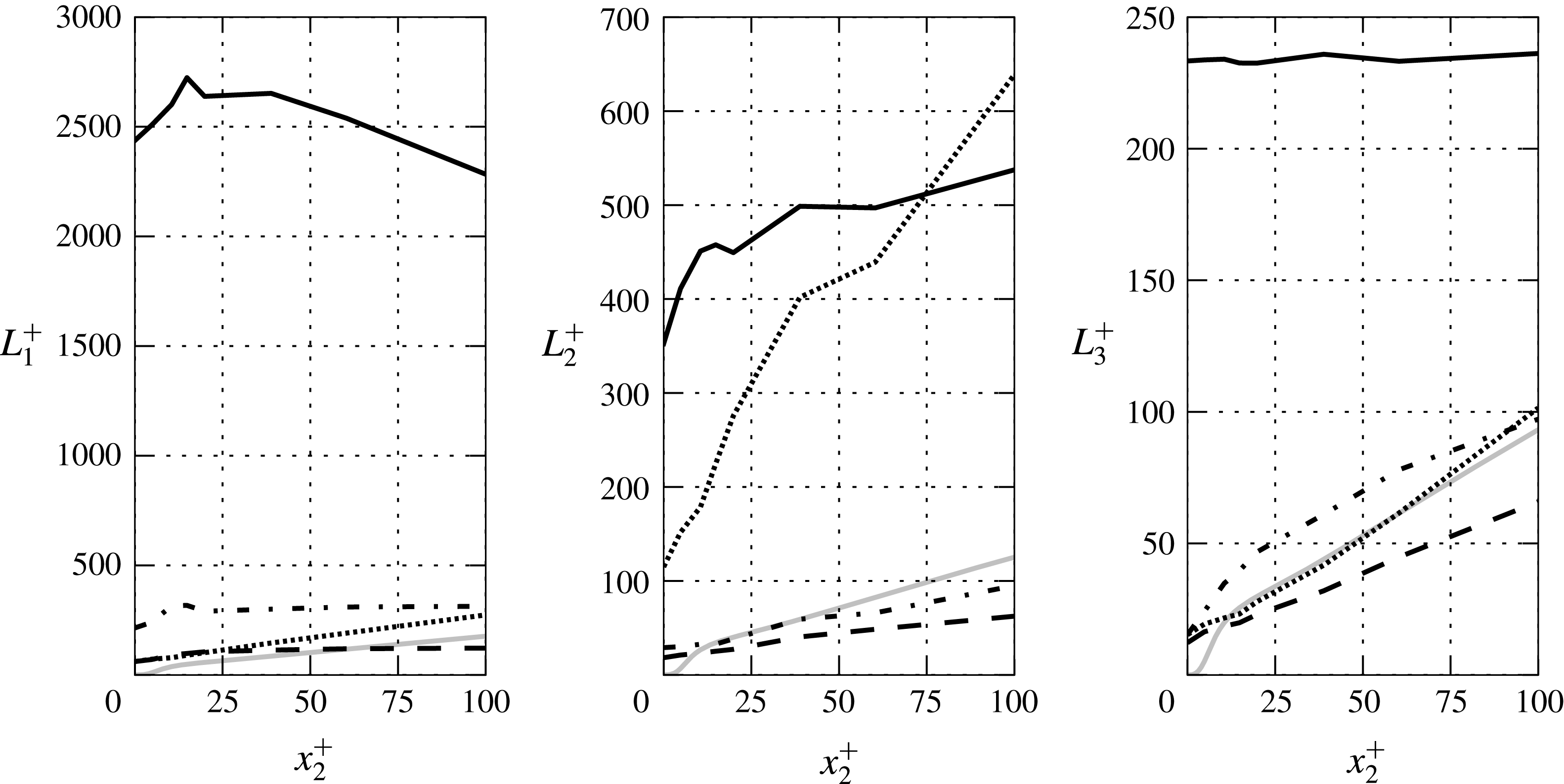
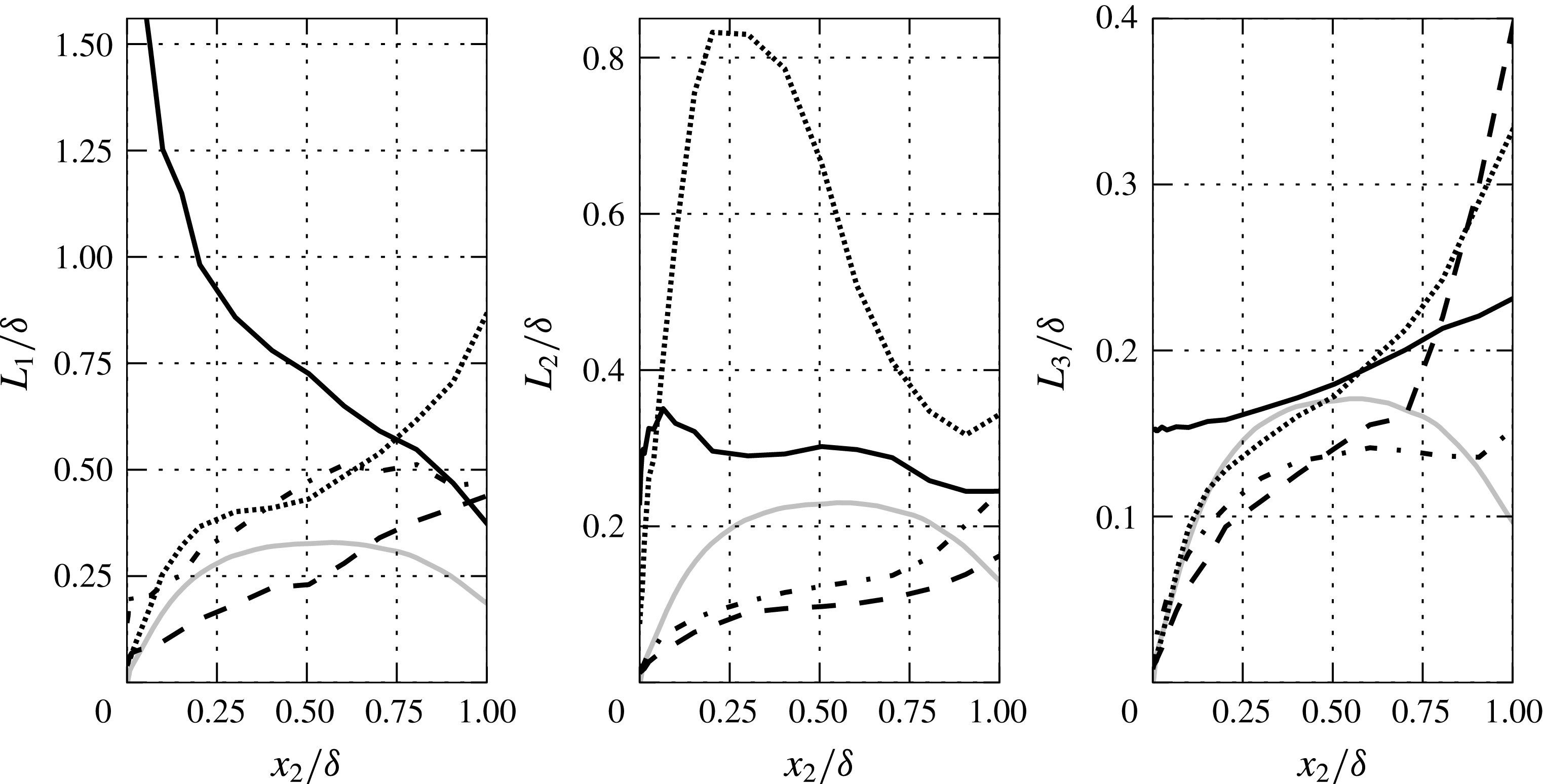
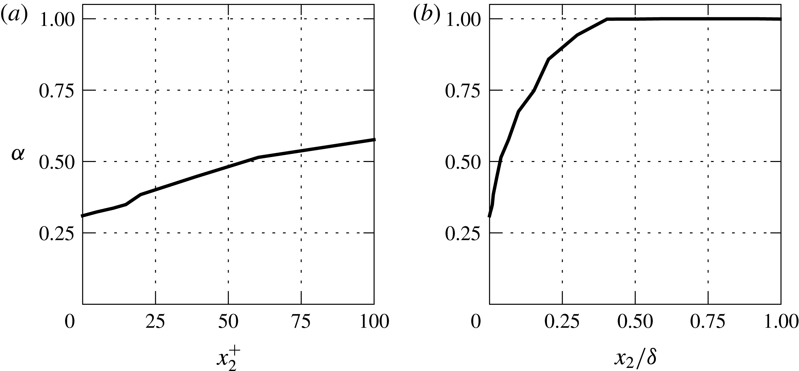
The evolutions of the parameter
 $\unicode[STIX]{x1D6FC}$
and the correlation lengths
 $L_{i}$
for each coefficient are presented in figures 6–8. These parameters are calibrated using the DNS data of Sillero et al. (Reference Sillero, Jiménez and Moser2014) for
 $Re_{\unicode[STIX]{x1D703}}\approx 4860$
, available at http://hal.dmt.upm.es/raw_database/Boundary_Layer/High-Reynolds/HR2-3D-Correlations. We use an inner and an outer regions, defined as
 $x_{2}^{+}\leqslant 100$
and
 $x_{2}^{+}>100$
, where the parameters are scaled with wall units and outer units respectively. The evolutions of equivalent correlation lengths for the SAM (
 $L_{i}\equiv 0.54\unicode[STIX]{x1D6FE}_{i}L_{u}$
) are also included in figures 6 and 7 (only for
 $\unicode[STIX]{x1D60A}_{11}$
). The evolutions of the EAM correlation lengths are very different from the SAM ones.
Correlation lengths for the EAM scaled in wall units (
 $x_{2}^{+}=x_{2}u_{\unicode[STIX]{x1D70F}}/\unicode[STIX]{x1D708}$
,
 $L_{i}^{+}=L_{i}u_{\unicode[STIX]{x1D70F}}/\unicode[STIX]{x1D708}$
): —— (black),
 $\unicode[STIX]{x1D60A}_{11}$
; - - -,
 $\unicode[STIX]{x1D60A}_{22}$
;
 $-\cdot -$
,
 $\unicode[STIX]{x1D60A}_{33}$
;
 $\cdots \cdots$
,
 $\tilde{\unicode[STIX]{x1D60A}}_{12}$
. The grey lines represent equivalent correlation lengths (
 $L_{i}\equiv 0.54\unicode[STIX]{x1D6FE}_{i}L_{u}$
) for the SAM for
 $\unicode[STIX]{x1D60A}_{11}$
.

Correlation lengths for the EAM scaled in outer units: —— (black),
 $\unicode[STIX]{x1D60A}_{11}$
; - - -,
 $\unicode[STIX]{x1D60A}_{22}$
;
 $-\cdot -$
,
 $\unicode[STIX]{x1D60A}_{33}$
;
 $\cdots \cdots$
,
 $\tilde{\unicode[STIX]{x1D60A}}_{12}$
. The grey lines represent equivalent correlation lengths (
 $L_{i}\equiv 0.54\unicode[STIX]{x1D6FE}_{i}L_{u}$
) for the SAM for
 $\unicode[STIX]{x1D60A}_{11}$
.

Parameter
 $\unicode[STIX]{x1D6FC}$
for the EAM scaled in wall units (a) and outer units (b).

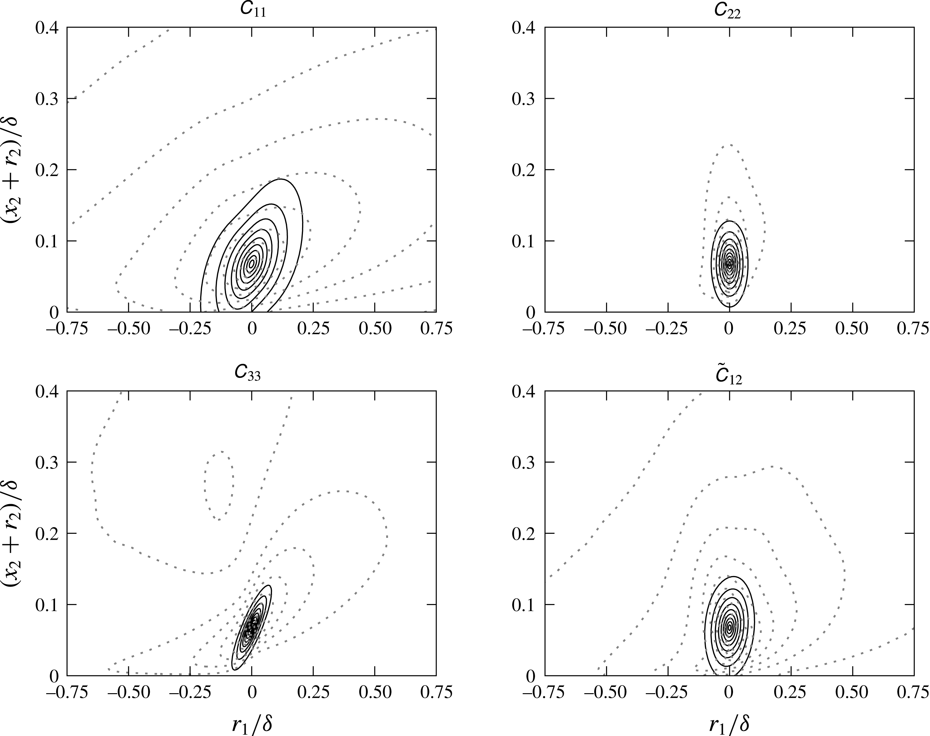
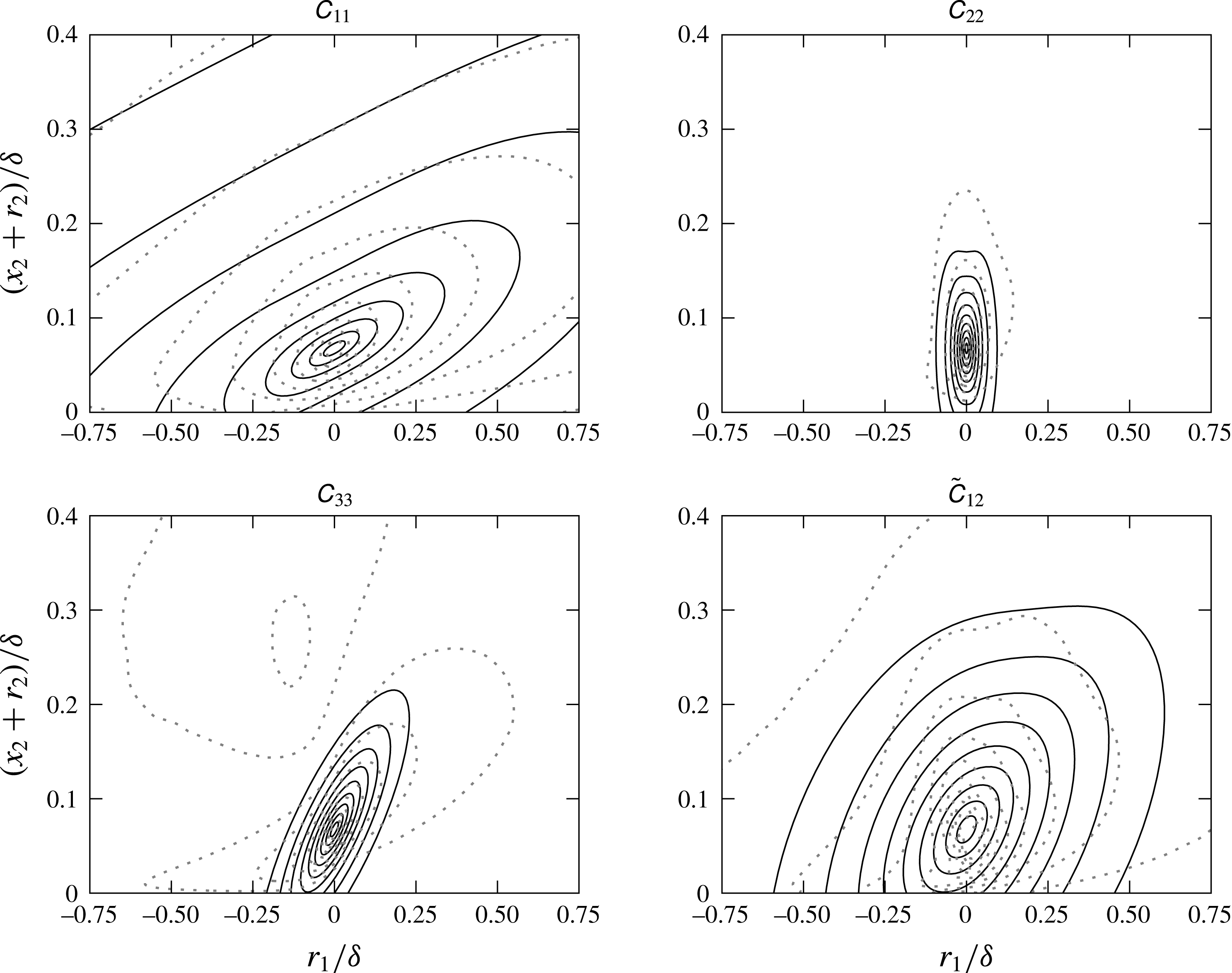
The results obtained with the EAM in the plane (
 $r_{1}$
,
 $r_{2}$
) are displayed in figure 9 where they are compared with the Sillero et al. (Reference Sillero, Jiménez and Moser2014) data. The size of the coefficients and their inclination angles appear to be more adapted, particularly for
 $\unicode[STIX]{x1D60A}_{11}$
. Nevertheless, some discrepancies are still visible for the other coefficients. For instance, these coefficients decay a little too quickly. As the other models, the EAM also fails to accurately take into account the decrease of the coefficient values close to the wall.
Streamwise (
 $r_{1}$
,
 $r_{2}$
) sections of the correlation coefficients obtained with the EAM for
 $r_{3}=0$
,
 $\unicode[STIX]{x0394}t=0$
,
 $x_{2}/\unicode[STIX]{x1D6FF}=0.065$
and
 $Re_{\unicode[STIX]{x1D703}}\approx 4860$
(the flow is from left to right). Positive contours (——) are from
 $0.1$
to
 $0.9$
with increments of
 $0.1$
. The grey dotted contours are the DNS results of Sillero et al. (Reference Sillero, Jiménez and Moser2014) at the same height and Reynolds number.

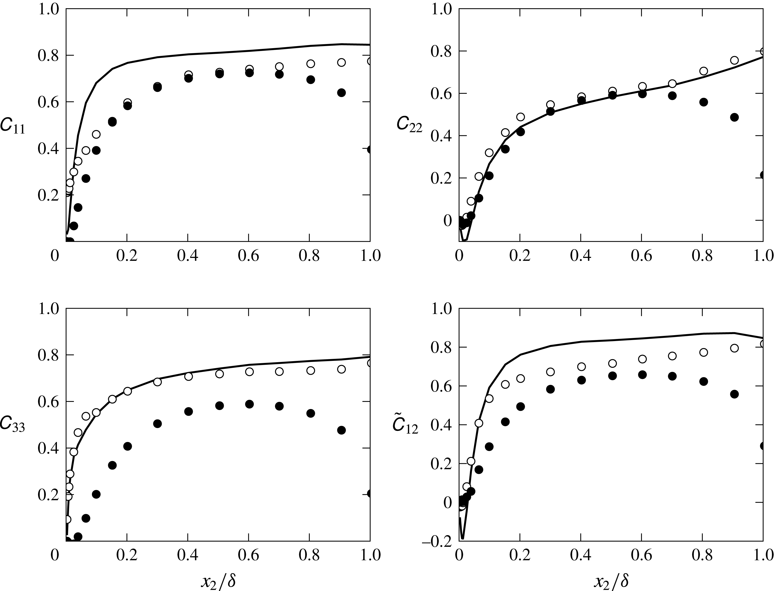
Figure 10 shows the evolution of the correlation coefficients, obtained with the EAM, the SAM and DNS data, with respect to
 $x_{2}$
for a fixed separation distance. The EAM results are better than the SAM ones for
 $\unicode[STIX]{x1D60A}_{33}$
and
 $\tilde{\unicode[STIX]{x1D60A}}_{12}$
. For
 $\unicode[STIX]{x1D60A}_{11}$
, both results are quite close for
 $0.2<x_{2}/\unicode[STIX]{x1D6FF}<0.6$
. For
 $x_{2}/\unicode[STIX]{x1D6FF}<0.2$
and
 $x_{2}/\unicode[STIX]{x1D6FF}>0.6$
, the coefficient
 $\unicode[STIX]{x1D60A}_{11}$
estimated with the EAM is closer to DNS data. For the
 $\unicode[STIX]{x1D60A}_{22}$
, the values obtained with the EAM are better for
 $x_{2}/\unicode[STIX]{x1D6FF}>0.6$
.
Evolution of the correlation coefficients with respect to
 $x_{2}$
for
 $\boldsymbol{r}=(0.030\unicode[STIX]{x1D6FF},0,0.037\unicode[STIX]{x1D6FF})$
,
 $\unicode[STIX]{x0394}t=0$
and
 $Re_{\unicode[STIX]{x1D703}}\approx 4860$
. For each panel: ——, DNS (Sillero et al.
Reference Sillero, Jiménez and Moser2014); ○, EAM; ●, SAM (
 $L=0.54L_{u}$
).

3.2.5 Model comparison
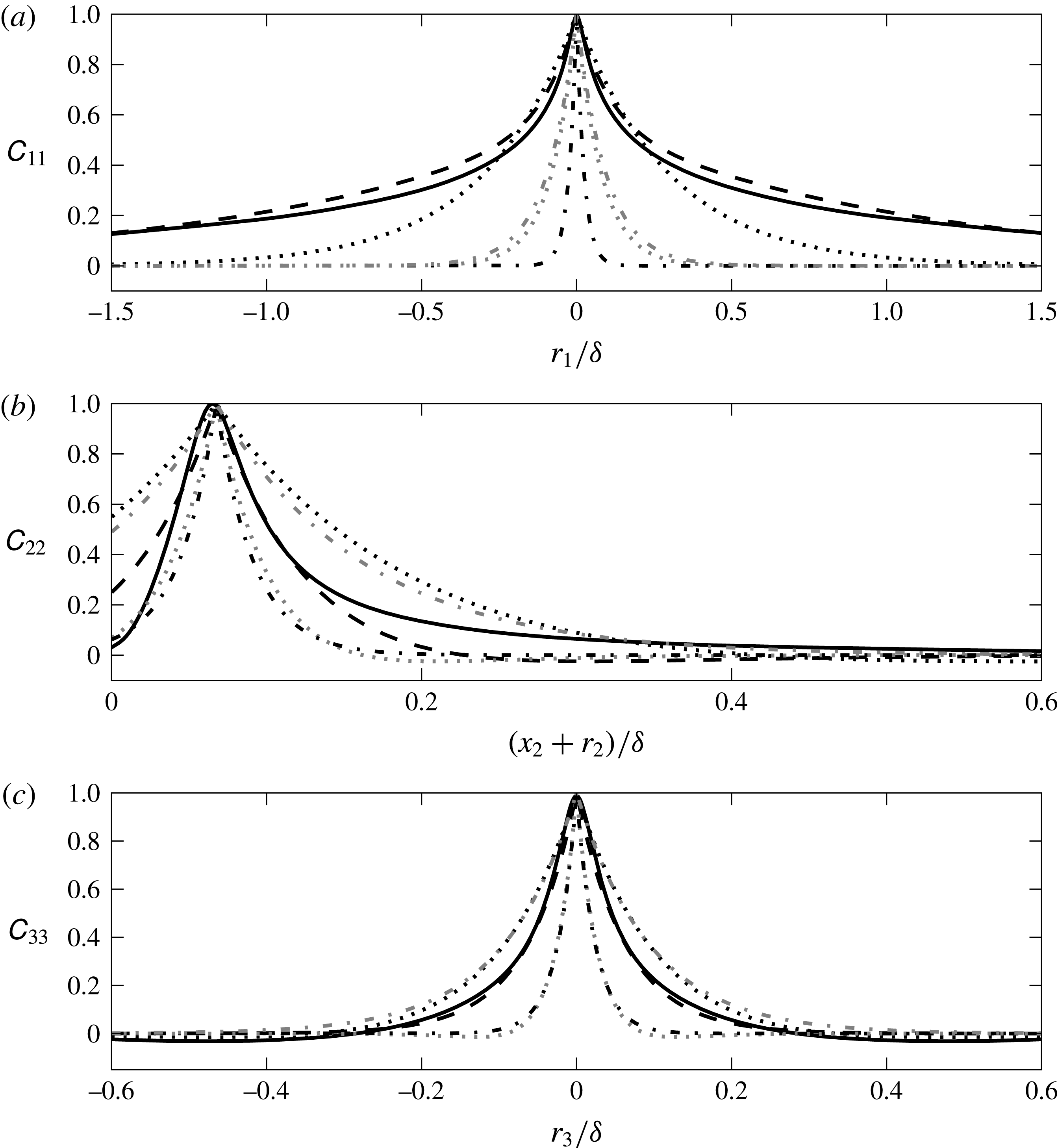
A comparison of the EAM, SAM and the isotropic model is presented in figure 11. Results are compared with the DNS data of Sillero et al. (Reference Sillero, Jiménez and Moser2014). As expected, the values obtained with the EAM are closer to the DNS data, particularly for
 $\unicode[STIX]{x1D60A}_{11}$
in the streamwise direction. The isotropic model and the SAM are not adapted for
 $\unicode[STIX]{x1D60A}_{11}$
in this direction. For
 $\unicode[STIX]{x1D60A}_{22}$
and
 $\unicode[STIX]{x1D60A}_{33}$
, all models have similar shapes but the scales are different. The results obtained with the isotropic model for
 $L=\unicode[STIX]{x1D706}_{f}$
and the SAM for
 $L=0.54L_{u}$
are too narrow whereas both models give correlations which are too wide for the other correlation lengths (
 $L=0.54L_{u}$
and
 $L=0.35\unicode[STIX]{x1D6FF}$
respectively).
Correlation coefficients evolution in one direction at
 $x_{2}/\unicode[STIX]{x1D6FF}=0.065$
and
 $Re_{\unicode[STIX]{x1D703}}\approx 4860$
. (a)
 $\unicode[STIX]{x1D60A}_{11}(x_{2},r_{1},0,0)$
; (b)
 $\unicode[STIX]{x1D60A}_{22}(x_{2},0,r_{2},0)$
; (c)
 $\unicode[STIX]{x1D60A}_{33}(x_{2},0,0,r_{3})$
. For each panel: ——, DNS (Sillero et al.
Reference Sillero, Jiménez and Moser2014); - - -, EAM;
 $-\cdot -$
, isotropic model (black,
 $L=\unicode[STIX]{x1D706}_{f}$
; grey,
 $L=0.54L_{u}$
);
 $\cdots \cdots$
, SAM (black,
 $L=0.35\unicode[STIX]{x1D6FF}$
; grey,
 $L=0.54L_{u}$
).

As shown in figures 3 and 11, the shape of the velocity correlation coefficients is complex and the ellipsoidal form of the model derived from the isotropic turbulence theory is not perfectly adapted, even with inclination angles. Some improvements involve more complex functions than the correlation functions
 $f$
and
 $g$
, in order to take into account the asymmetry of the correlations for separations in the normal direction. However, this is far beyond the scope of the present work. Further comparisons of the
 $\unicode[STIX]{x1D60A}_{ij}$
models are made in § 4.2 where their influence on the pressure frequency spectrum is discussed.
3.3 Space–time correlations model
Several theories and models exist for turbulent space–time velocity correlations (see the reviews of Wallace (Reference Wallace2014) and He, Jin & Yang (Reference He, Jin and Yang2017)). In this work, we compare two models which relate spatial correlations to space–time correlations.
The first one is Taylor’s frozen turbulence hypothesis (Taylor Reference Taylor1938), stating that turbulent structures are carried past a fixed point by the mean flow at the convection velocity
 $U_{c}$
without any major changes. With this hypothesis, space–time velocity correlations for a spatial separation
 $r_{1}$
in the streamwise direction and a time separation
 $\unicode[STIX]{x0394}t$
can be written:
 $$\begin{eqnarray}\unicode[STIX]{x1D619}_{ij}(\boldsymbol{x},r_{1},\unicode[STIX]{x0394}t)=\unicode[STIX]{x1D619}_{ij}(\boldsymbol{x},r_{1}-U_{c}\unicode[STIX]{x0394}t,0).\end{eqnarray}$$
According to He & Zhang (Reference He and Zhang2006), Taylor’s frozen flow hypothesis is only a first approximation which has limitations. Indeed, with this hypothesis, iso-correlation contours of
 $\unicode[STIX]{x1D619}_{ij}(\boldsymbol{x},r_{1},\unicode[STIX]{x0394}t)$
are straight lines and thus the correlations remain constant even for large values of
 $r_{1}$
and
 $\unicode[STIX]{x0394}t$
. This result is not consistent because correlation functions decrease with increasing space and time separations. Moreover, several simulations and experiments (He & Zhang Reference He and Zhang2006; Guo et al.
Reference Guo, Li, Zhang and He2012; Wallace Reference Wallace2014; Wang, Guan & Jiang Reference Wang, Guan and Jiang2014) show that the iso-correlation contours are not straight lines but elongated ellipses. Nevertheless, Taylor’s hypothesis is often used (Panton & Linebarger Reference Panton and Linebarger1974; Lee et al.
Reference Lee, Blake and Farabee2005; Bertagnolio et al.
Reference Bertagnolio, Fischer and Jun Zhu2014) due to its simplicity and ease of implementation.
The elliptic model of He & Zhang (Reference He and Zhang2006) is formulated using a second-order Taylor series expansion of
 $\unicode[STIX]{x1D619}_{ij}(\boldsymbol{x},r_{1},\unicode[STIX]{x0394}t)$
. This model relates space correlation to space–time correlations via two parameters, the convection velocity
 $U_{c}$
and a velocity
 $V$
which characterizes the distortion of small-scale eddies:
 $$\begin{eqnarray}\unicode[STIX]{x1D619}_{ij}(\boldsymbol{x},r_{1},\unicode[STIX]{x0394}t)=\unicode[STIX]{x1D619}_{ij}\left(\boldsymbol{x},\sqrt{(r_{1}-U_{c}\unicode[STIX]{x0394}t)^{2}+V^{2}\unicode[STIX]{x0394}t^{2}},0\right).\end{eqnarray}$$
The iso-correlation contours obtained with this model are elliptic. Contrary to Taylor’s hypothesis, the elliptic model also takes into account the decorrelation induced by the random sweeping of velocity fluctuations and the shearing of mean flows which distort small-scale eddies (He et al. Reference He, Jin and Yang2017). This model was successfully applied by Zhao & He (Reference Zhao and He2009) and Guo et al. (Reference Guo, Li, Zhang and He2012) for turbulent channel flows and by Wang et al. (Reference Wang, Guan and Jiang2014) for a TBL flow.
Two different models for the convection velocity are considered. The first one is
 $U_{c}=0.7U_{\infty }$
. Taking a uniform value for the convection velocity is mainly motivated here by its simplicity and ease of implementation. The value
 $U_{c}=0.7U_{\infty }$
is moreover justified by the DNS results of Choi & Moin (Reference Choi and Moin1990), in which it is shown that this value constitutes a reasonable approximation. In more recent efforts, del Álamo & Jiménez (Reference del Álamo and Jiménez2009) demonstrate that a uniform convection velocity is not accurate since the convection velocity is a function of the eddy frequency and of their wall distance. Therefore, a second model, taken from Renard & Deck (Reference Renard and Deck2015) results for a global correlation-based convection velocity, is evaluated. They obtained a convection velocity which is a function of the wall distance
 $x_{2}$
and is close to the mean velocity except near the wall where it is larger and nearly constant. There are other models available in the literature for
 $U_{c}$
, particularly expressions which are functions of the frequency (e.g. Wills Reference Wills1971; Panton & Linebarger Reference Panton and Linebarger1974). However their implementation in our space–time correlation model is not straightforward so they are not studied in the present work.
For
 $V$
, we use the expression proposed by Monté (Reference Monté2013) which defines a velocity
 $V$
for each coefficient
 $\unicode[STIX]{x1D60A}_{ij}$
:
 $$\begin{eqnarray}\unicode[STIX]{x1D61D}_{ij}^{2}(\boldsymbol{x})=\unicode[STIX]{x1D61A}_{ij}^{2}(\boldsymbol{x})\unicode[STIX]{x1D706}_{ij}^{2}(\boldsymbol{x})+\overline{u_{i}u_{j}}(\boldsymbol{x}),\end{eqnarray}$$
where
 $\unicode[STIX]{x1D61A}_{ij}$
is the mean rate-of-strain tensor and
 $\unicode[STIX]{x1D706}_{ij}$
is a Taylor scale defined from Reynolds stresses as:
 $\unicode[STIX]{x1D706}_{ij}=\sqrt{15|\overline{u_{i}u_{j}}|\unicode[STIX]{x1D708}/\unicode[STIX]{x1D700}}$
.
The influence of the space–time model on the pressure spectrum is discussed in § 4.2.
3.4 Kriging-based elliptic extended anisotropic model
In this work, the EAM and the elliptic model are used to close (2.7). The whole approach to compute the pressure correlations with the numerical method described in § 2.3 is referred to as the Kriging-based elliptic extended anisotropic model (KEEAM). In the following section, the influence of the closure model on the pressure spectrum is discussed. Then the KEEAM is compared to a few models presented in the introduction.
4 Results
4.1 RANS simulation
The RANS data used in this work were generated with the open-source computational fluid dynamics software Code_Saturne developed by EDF R&D (Archambeau, Méchitoua & Sakiz Reference Archambeau, Méchitoua and Sakiz2004). The elliptic blending Reynolds stress model (EBRSM) (Manceau & Hanjalić Reference Manceau and Hanjalić2002) is used for the turbulence closure. With this model, the value of
 $x_{2}^{+}=u_{\unicode[STIX]{x1D70F}}x_{2}/\unicode[STIX]{x1D708}$
for the first cell adjacent to the wall must be lower than 1. Therefore wall functions are not used and the equations are solved in all regions of the boundary layer.
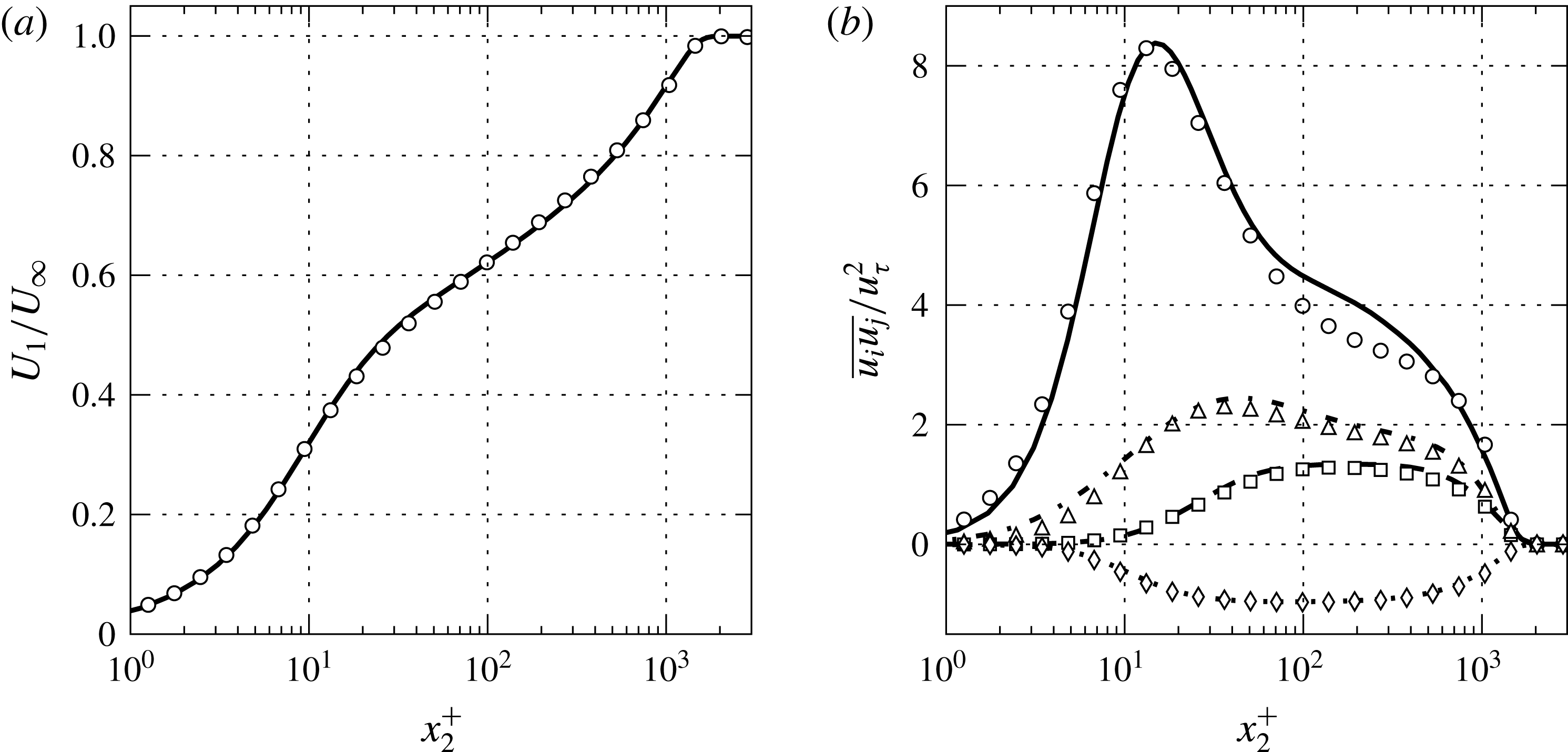
In figure 12, the mean streamwise velocity and the Reynolds stress profiles obtained with the EBRSM are compared with the DNS results of Sillero, Jiménez & Moser (Reference Sillero, Jiménez and Moser2013) at the same Reynolds number. The agreement of the data are satisfactory although there are slight differences for the streamwise and the spanwise Reynolds stresses.
(a) Mean streamwise velocity profile at
 $Re_{\unicode[STIX]{x1D703}}\approx 4860$
. ——, DNS data;
 $\circ$
, RANS data. (b) Reynolds stress profiles at
 $Re_{\unicode[STIX]{x1D703}}\approx 4860$
. Lines are DNS data and symbols are RANS data. —— and ○,
 $\overline{u_{1}u_{1}}$
; - - - and ▫,
 $\overline{u_{2}u_{2}}$
;
 $-\cdot -$
and ▵,
 $\overline{u_{3}u_{3}}$
;
 $\cdots \cdots$
and ♢,
 $\overline{u_{1}u_{2}}$
.

4.2 Frequency spectrum of the wall pressure fluctuations
4.2.1 Validation of the adaptive sampling method
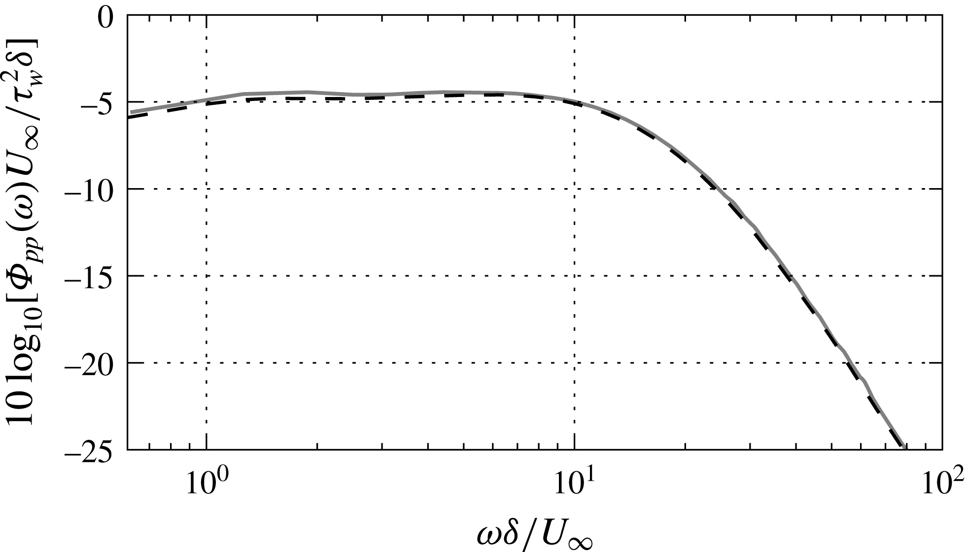
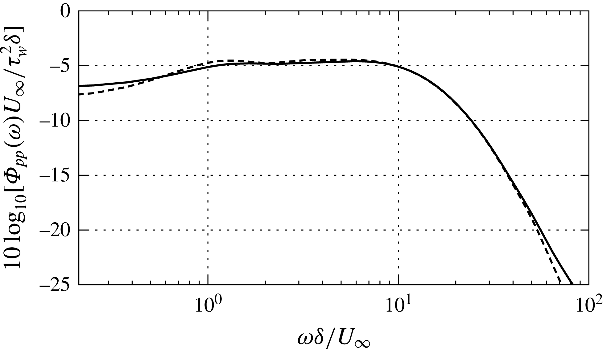
In order to validate the adaptive sampling strategy, the wall pressure frequency spectrum is computed with and without Kriging. The elliptic model with
 $U_{c}=0.7U_{\infty }$
and the EAM are used. The results are presented in figure 13. The spectrum without Kriging is computed with
 $1024$
values of the pressure time correlations whereas only
 $77$
points are necessary to obtain very satisfactory results with Kriging.
Frequency spectrum of the wall pressure fluctuations at
 $Re_{\unicode[STIX]{x1D703}}\approx 4860$
. ——, without Kriging; - - -, with Kriging.

4.2.2 Influence of the velocity correlation coefficient model
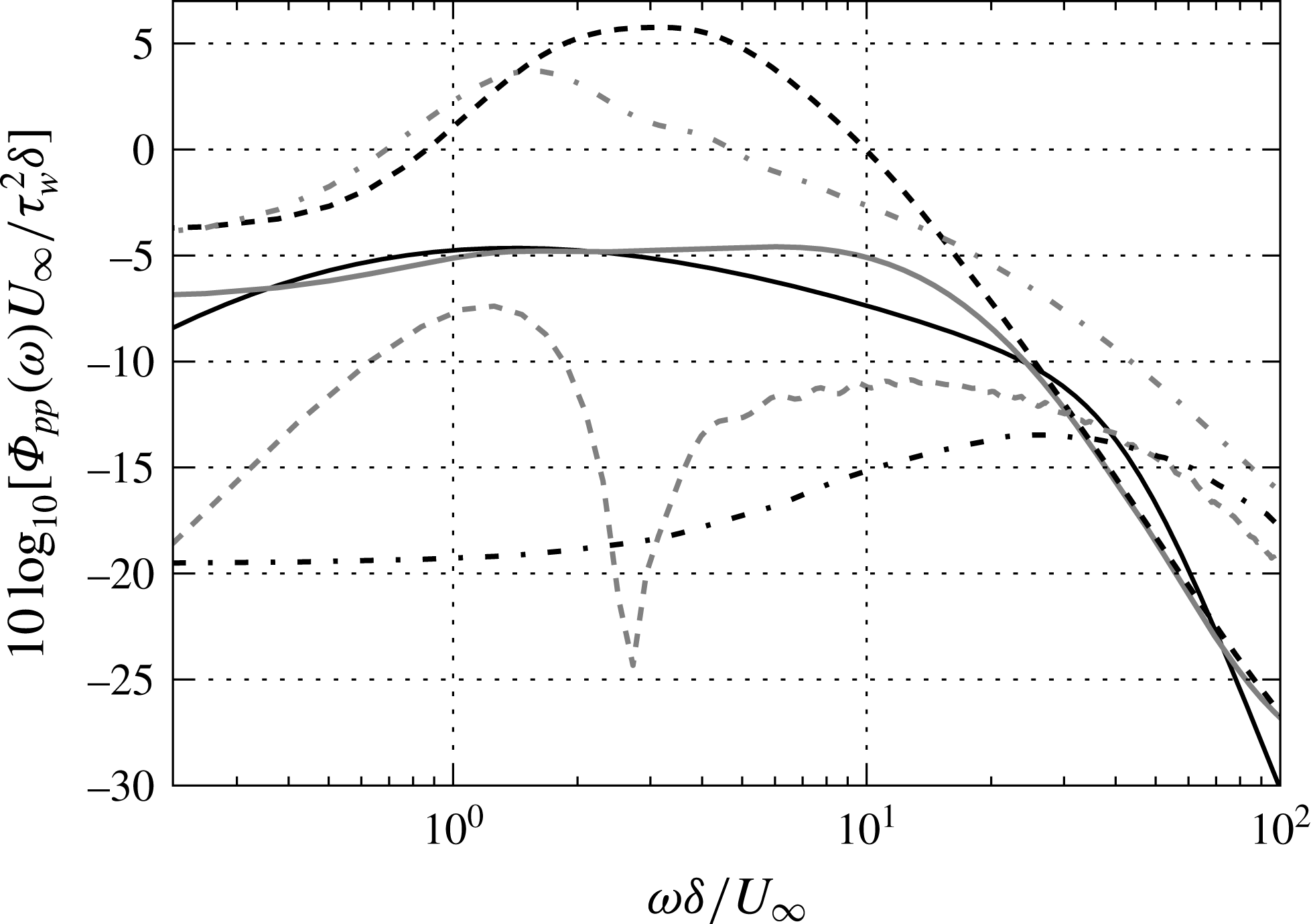
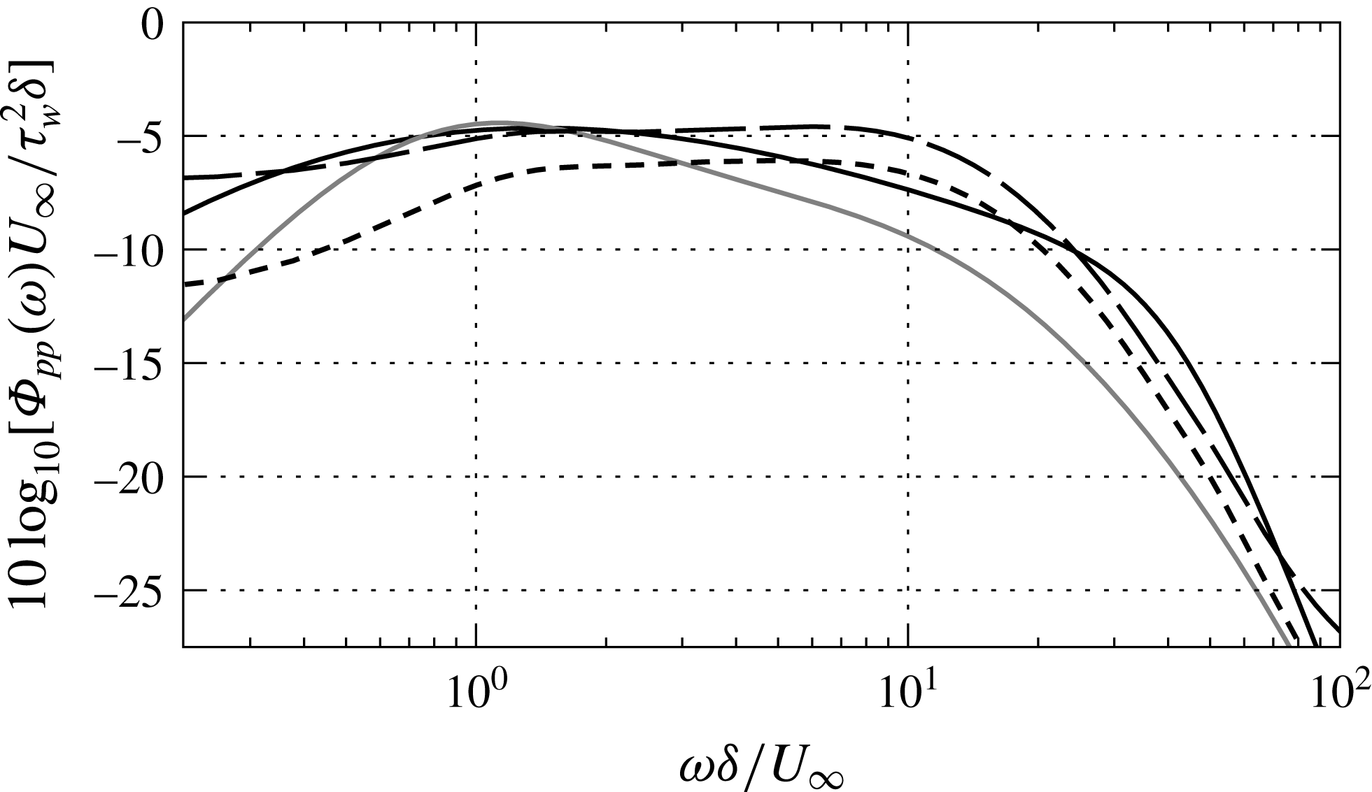
Wall pressure frequency spectra obtained with the different velocity correlation coefficient models previously described are presented in figure 14. The elliptic model is used to relate spatial correlations to space–time correlations. The Goody (Reference Goody2004) spectrum is also plotted as a reference since it provides satisfactory predictions of the frequency spectrum for a TBL flow over a flat plate (Hwang et al.
Reference Hwang, Bonness and Hambric2009). Large discrepancies can be observed between the pressure spectra, which shows the strong influence of the correlation coefficients. The choice of the correlation length
 $L$
has also a great influence for the SAM and the isotropic model. The wall pressure fluctuations estimated with the EAM are satisfactory in the whole frequency range.
Frequency spectrum of the wall pressure fluctuations at
 $Re_{\unicode[STIX]{x1D703}}\approx 4860$
. —— black, Goody (Reference Goody2004) model; —— grey, EAM;
 $-\cdot -$
, isotropic (black,
 $L=\unicode[STIX]{x1D706}_{f}$
; grey,
 $L=0.54L_{u}$
); - - -, SAM (black,
 $L=0.35\unicode[STIX]{x1D6FF}$
; grey,
 $L=0.54L_{u}$
).

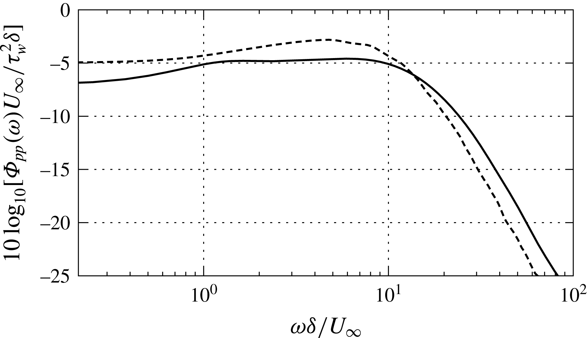
The influence of the space–time model (Taylor’s hypothesis or the elliptic model) and the convection velocity model are also studied. The frequency spectra computed with the EAM are shown in figure 15. The pressure spectra obtained with Taylor’s hypothesis and the elliptic model are very close, except at low frequencies and very high frequencies. However, for the wavenumber–frequency spectrum, Taylor’s hypothesis leads to a Dirac delta function so the elliptic model is used in the KEEAM. The convection velocity model has more influence on the form of the pressure spectrum (see figure 16): the pressure levels obtained with
 $U_{c}(x_{2})$
are larger and the spectrum decay at a lower frequency. The spectrum computed with
 $U_{c}=0.7U_{\infty }$
is thus in better agreement with Goody (Reference Goody2004) model, so this expression is retained for the rest of the study.
Frequency spectrum of the wall pressure fluctuations at
 $Re_{\unicode[STIX]{x1D703}}\approx 4860$
(
 $U_{c}=0.7U_{\infty }$
). ——, elliptic model; - - -, Taylor’s hypothesis.

Frequency spectrum of the wall pressure fluctuations at
 $Re_{\unicode[STIX]{x1D703}}\approx 4860$
. ——,
 $U_{c}=0.7U_{\infty }$
; - - -,
 $U_{c}(x_{2})$
.

4.2.3 TMS and TT contributions
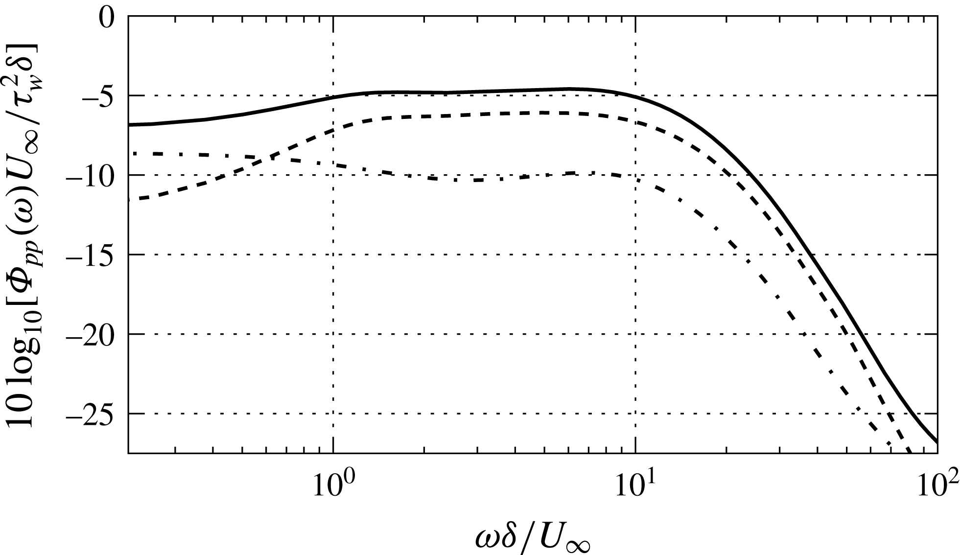
The wall pressure spectra with the TMS and TT terms contributions are displayed in figure 17. The magnitude of the TT spectrum is lower than the TMS one, except at low frequencies. This is consistent with Kraichnan (Reference Kraichnan1956) and Remmler et al. (Reference Remmler, Christophe, Anthoine and Moreau2010). However, depending on the precision required, the TT terms should not be neglected at mid frequencies. These results differ from the Chang et al. (Reference Chang, Piomelli and Blake1999) results for the streamwise wavenumber pressure spectrum of a fully developed turbulent channel flow at a low Reynolds number. They observed that the TMS and TT terms are of the same order but that the TMS term is greater for the whole streamwise wavenumber range.
Frequency spectrum of the wall pressure fluctuations computed with the KEEAM at
 $Re_{\unicode[STIX]{x1D703}}\approx 4860$
. ——, total; - - -, TMS;
 $-\cdot -$
, TT.

4.2.4 Influence of the Reynolds number
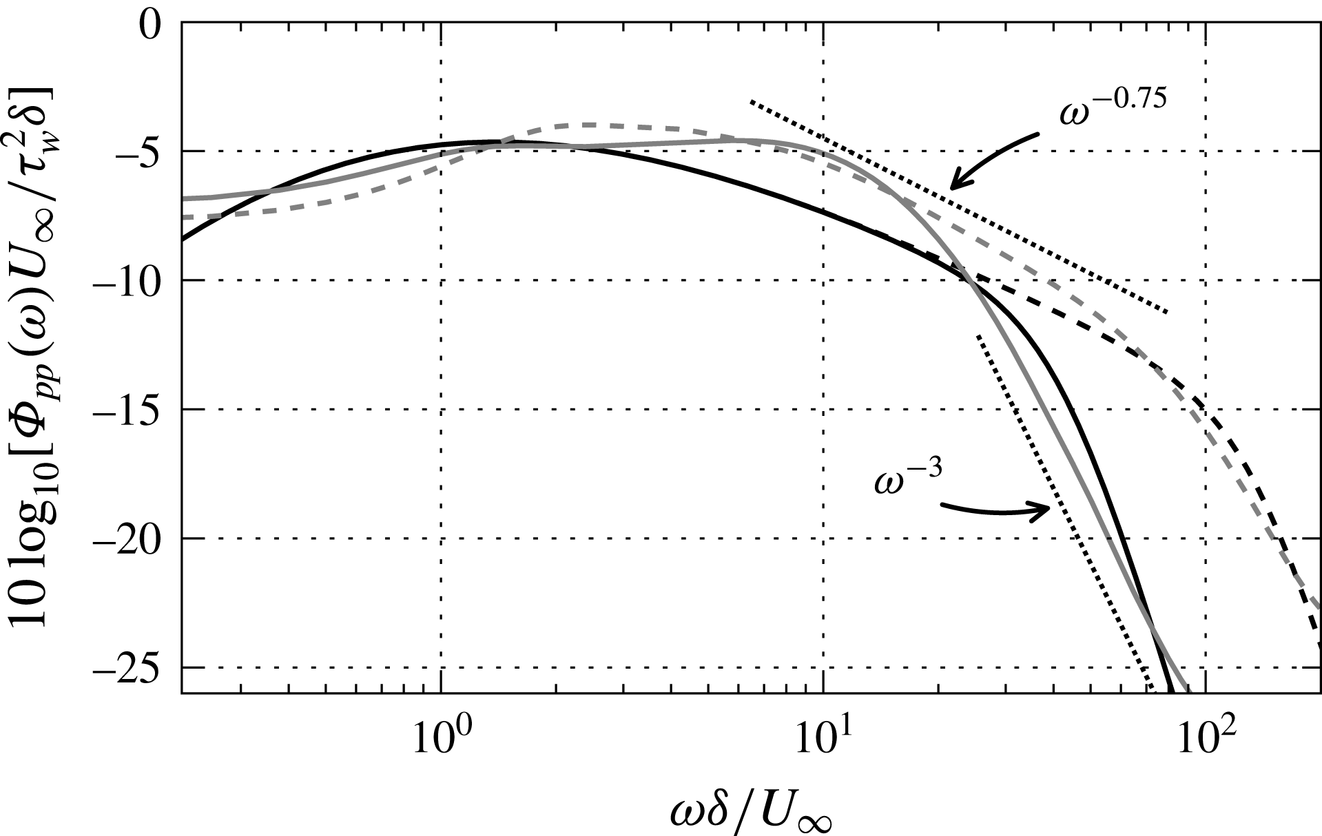
The frequency pressure spectra obtained with the KEEAM at two Reynolds numbers are presented in figure 18. They are compared to the Goody (Reference Goody2004) model which is based on experimental pressure spectra measurements on a large range of Reynolds numbers. Since it takes into account the effect of the Reynolds number, it is also used as a reference here. The wall pressure spectra are in agreement with the Goody (Reference Goody2004) model at both Reynolds numbers. It shows that the present model is also able to take accurately into account the influence of the Reynolds number even if the parameters of the EAM were calibrated with DNS results for a particular Reynolds number. Other predictions of the pressure spectrum were performed with the KEEAM and it gives accurate results (compared to Goody model) for
 $3\times 10^{3}<Re_{\unicode[STIX]{x1D703}}<3\times 10^{4}$
.
The wall pressure levels predicted by the KEEAM are quite close to the ones obtained with Goody model but there are differences. Indeed, the maximum of the KEEAM spectra are reached at higher frequencies. In the high frequency region, the spectrum evolves as
 $\unicode[STIX]{x1D714}^{-3}$
whereas Goody model is designed to reproduce a
 $-5$
slope. According to Blake (Reference Blake1986), the decay rate of the spectrum in this range is due to contributions from the viscous wall region. The EAM could be improved in this area. For
 $Re_{\unicode[STIX]{x1D703}}\approx 4860$
, the KEEAM does not predict the universal region, characterized by a slope between
 $-0.7$
and
 $-1.11$
(Smol’yakov Reference Smol’yakov2000; Goody Reference Goody2004). However, this region is visible for
 $Re_{\unicode[STIX]{x1D703}}\approx 21100$
with a
 $-0.75$
slope, which is close to the
 $-0.7$
slope of the Goody spectrum. So the KEEAM reproduced the universal region but it appears at a higher Reynolds number.
Frequency spectra of the wall pressure fluctuations computed at two different Reynolds numbers. Black lines are Goody (Reference Goody2004) model and grey lines are the KEEAM. ——,
 $Re_{\unicode[STIX]{x1D703}}\approx 4860$
; - - -,
 $Re_{\unicode[STIX]{x1D703}}\approx 21100$
.

4.2.5 Comparison with a spectral formulation of the wall pressure
Besides the Goody (Reference Goody2004) model, the wall pressure spectrum computed is also compared to the model of Bertagnolio et al. (Reference Bertagnolio, Fischer and Jun Zhu2014) which uses a spectral solution to the Poisson equation (see table 2). Using Taylor’s frozen flow hypothesis, the frequency pressure spectrum is given by:
 $$\begin{eqnarray}\unicode[STIX]{x1D6F7}_{pp}(\unicode[STIX]{x1D714})=\int _{-\infty }^{\infty }\int _{0}^{\infty }\frac{4\unicode[STIX]{x1D70C}^{2}}{U_{c}}L_{2}(x_{2})\overline{u_{2}u_{2}}\left(\frac{\unicode[STIX]{x2202}U_{1}}{\unicode[STIX]{x2202}x_{2}}\right)^{2}\frac{k_{c}^{2}}{k^{2}}\unicode[STIX]{x1D6F7}_{22}(k_{c},k_{3})\text{e}^{-2kx_{2}}\,\text{d}x_{2}\,\text{d}k_{3},\end{eqnarray}$$
with:
 $$\begin{eqnarray}\displaystyle & \displaystyle \unicode[STIX]{x1D6F7}_{22}(k_{1},k_{3})=\frac{4}{9\unicode[STIX]{x03C0}}\frac{\unicode[STIX]{x1D6FD}_{1}\unicode[STIX]{x1D6FD}_{3}}{k_{e}^{2}}\frac{(\unicode[STIX]{x1D6FD}_{1}k_{1}/k_{e})^{2}+(\unicode[STIX]{x1D6FD}_{3}k_{3}/k_{e})^{2}}{[1+(\unicode[STIX]{x1D6FD}_{1}k_{1}/k_{e})^{2}+(\unicode[STIX]{x1D6FD}_{3}k_{3}/k_{e})^{2}]^{7/3}} & \displaystyle\end{eqnarray}$$
 $$\begin{eqnarray}\displaystyle & \displaystyle k=\sqrt{k_{c}^{2}+k_{3}^{2}} & \displaystyle\end{eqnarray}$$
 $$\begin{eqnarray}\displaystyle & \displaystyle L_{2}=0.747\unicode[STIX]{x1D6EC} & \displaystyle\end{eqnarray}$$
 $$\begin{eqnarray}\displaystyle & \displaystyle \unicode[STIX]{x1D6EC}=0.519\frac{{\mathcal{K}}^{3/2}}{\unicode[STIX]{x1D700}} & \displaystyle\end{eqnarray}$$
 $$\begin{eqnarray}\displaystyle & \displaystyle k_{e}=\frac{1}{2\unicode[STIX]{x1D6EC}} & \displaystyle\end{eqnarray}$$
 $$\begin{eqnarray}\displaystyle & \displaystyle \unicode[STIX]{x1D6FD}_{i}=\frac{\overline{u_{i}u_{i}}}{\overline{u_{1}u_{1}}}. & \displaystyle\end{eqnarray}$$
Since the Bertagnolio et al. (Reference Bertagnolio, Fischer and Jun Zhu2014) expressions for
 $\unicode[STIX]{x1D6FD}_{1}$
and
 $\unicode[STIX]{x1D6FD}_{3}$
are not adapted for TBL flows without pressure gradient, we use the ones proposed by Stalnov, Paruchuri & Joseph (Reference Stalnov, Paruchuri and Joseph2015) instead. We also use their relation for
 $k_{e}$
which is expected to be more accurate. The mean velocity field and the Reynolds stresses are obtained from RANS solutions. A comparison of the frequency pressure spectra is presented in figure 19. Discrepancies can be observed between the Goody (Reference Goody2004) and Bertagnolio et al. (Reference Bertagnolio, Fischer and Jun Zhu2014) models. The differences at low frequencies are expected since only the TMS term is taken into account in the latter model. Large discrepancies can also be observed between the TMS spectrum computed with the KEEAM and the Bertagnolio et al. (Reference Bertagnolio, Fischer and Jun Zhu2014) model.
Frequency spectra of the wall pressure fluctuations at
 $Re_{\unicode[STIX]{x1D703}}\approx 4860$
. Black ——, Goody (Reference Goody2004); grey ——, Bertagnolio et al. (Reference Bertagnolio, Fischer and Jun Zhu2014); — —, KEEAM (total); - - -, KEEAM (TMS).

4.3 Wavenumber–frequency spectrum of the wall pressure fluctuations
In the present work, the pressure correlations
 $R_{pp}(r_{s1},0,\unicode[STIX]{x0394}t)$
are computed as well as the streamwise wavenumber–frequency spectrum which is given by:
 $$\begin{eqnarray}\displaystyle \unicode[STIX]{x1D6F7}(k_{1},\unicode[STIX]{x1D714}) & = & \displaystyle \frac{1}{(2\unicode[STIX]{x03C0})^{2}}\int _{-\infty }^{\infty }\int _{-\infty }^{\infty }R_{pp}(r_{s1},0,\unicode[STIX]{x0394}t)\text{e}^{-\text{i}(k_{1}r_{s1}+\unicode[STIX]{x1D714}\unicode[STIX]{x0394}t)}\,\text{d}r_{s1}\,\text{d}\unicode[STIX]{x0394}t\nonumber\\ \displaystyle & = & \displaystyle \int _{-\infty }^{\infty }\unicode[STIX]{x1D6F7}(k_{1},k_{3},\unicode[STIX]{x1D714})\,\text{d}k_{3}.\end{eqnarray}$$
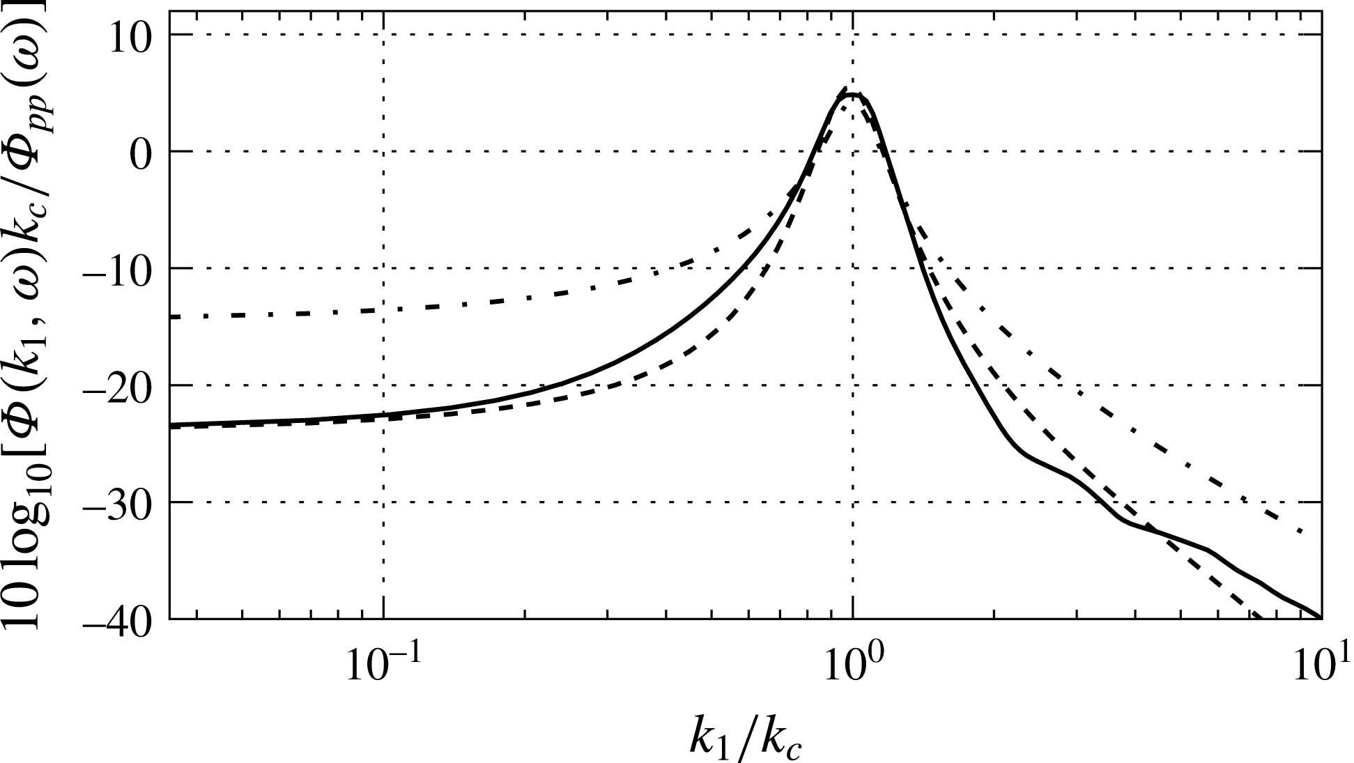
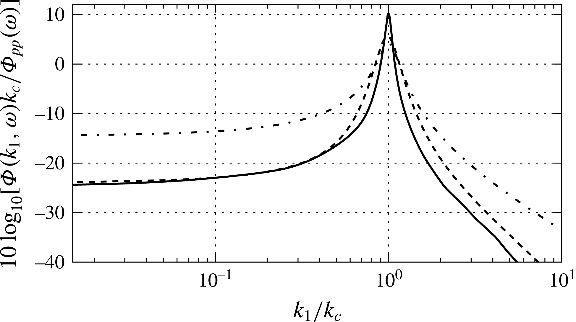
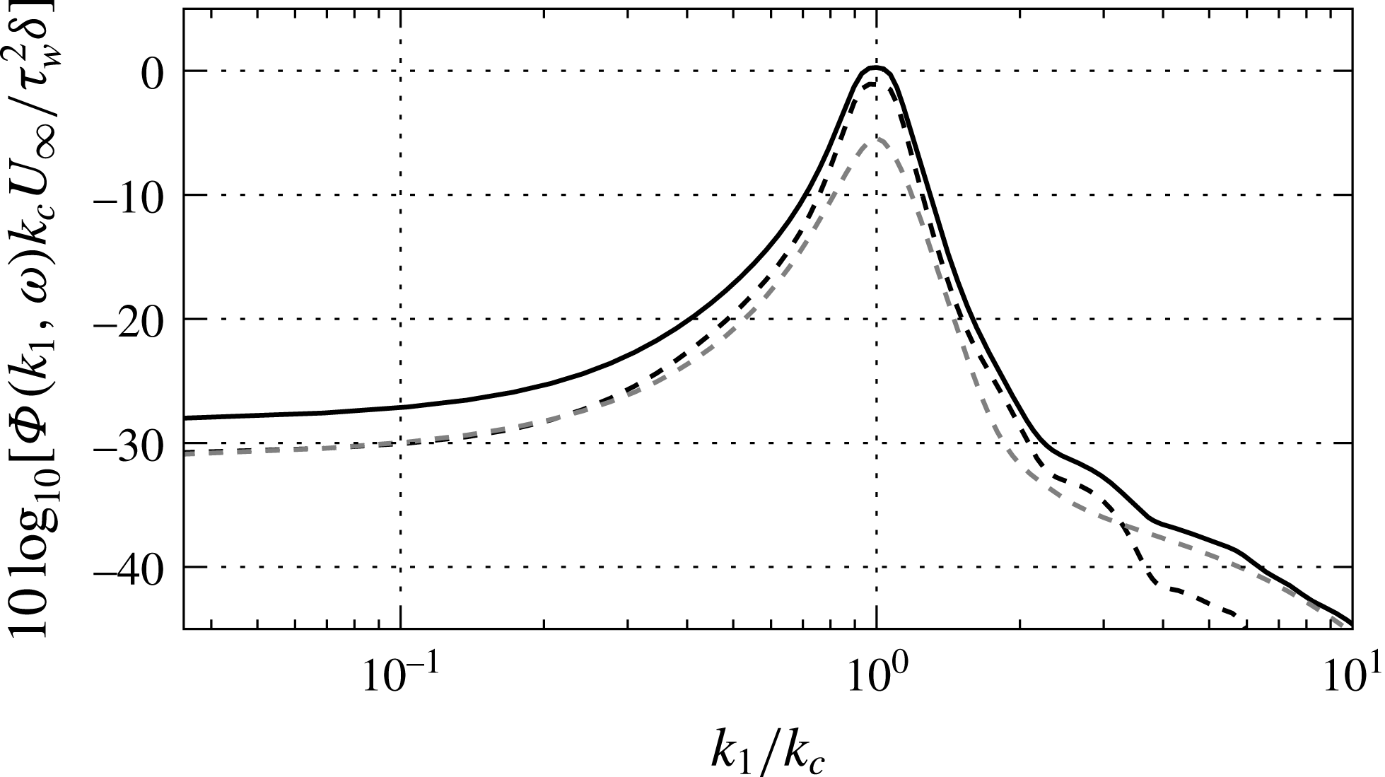
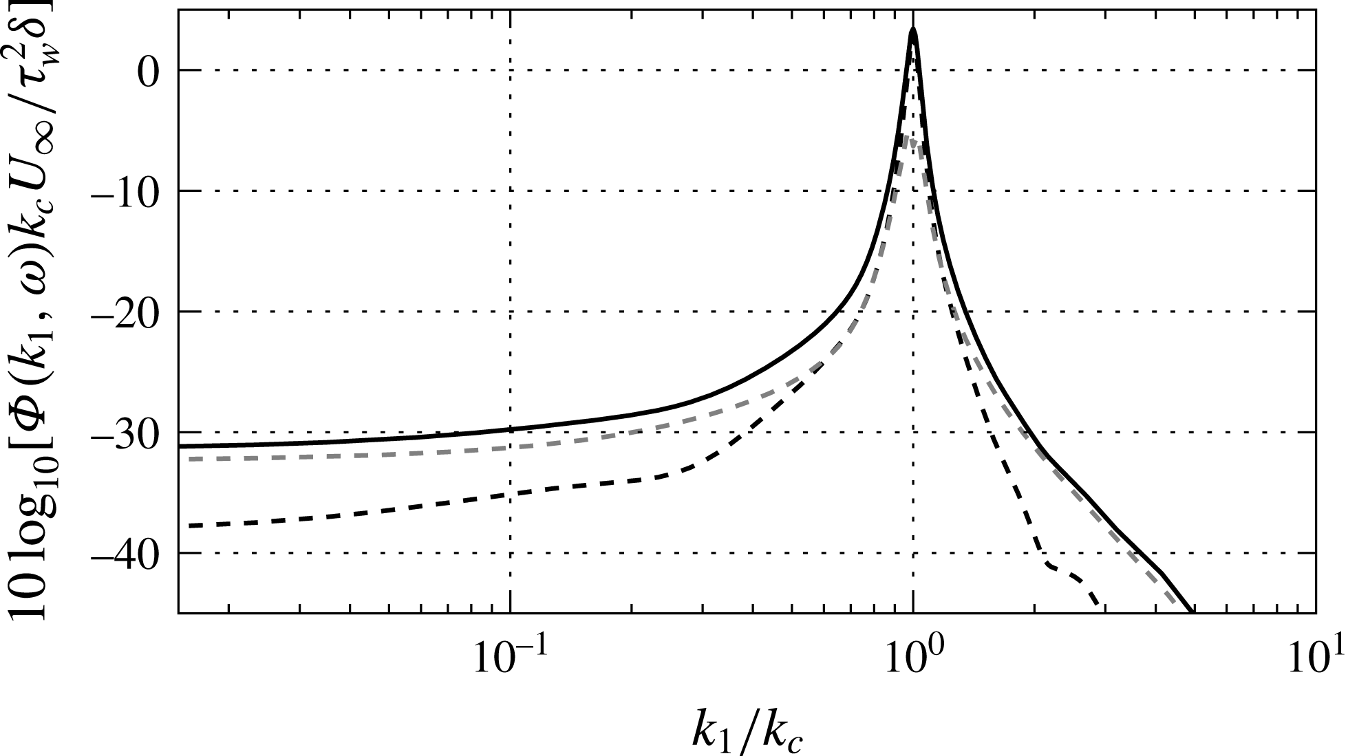
The results, presented in figures 20 and 21, are compared to the empirical models of Corcos (Reference Corcos1964) and Chase (Reference Chase1987) (integrated over
 $k_{3}$
) at two frequencies. The KEEAM is able to predict a convective peak whose amplitude is in agreement with both empirical models. It also predicts a subconvective plateau that is close to the one obtained with the Chase (Reference Chase1987) model. As mentioned before, large discrepancies exist between the empirical models in the subconvective range and there is no consensus on their validity. Nevertheless, the Corcos (Reference Corcos1964) model is known to overestimate the pressure spectrum at low wavenumbers (Bonness et al.
Reference Bonness, Capone and Hambric2010).
Figures 22 and 23 show the corresponding TMS and TT contributions for the spectrum obtained with the KEEAM. Around the convective peak, the TT terms are lower than the TMS one at both frequencies. On the contrary, in the viscous region the TT terms dominate. In the subconvective range, the TMS and TT contributions are of the same order for
 $\unicode[STIX]{x1D714}\unicode[STIX]{x1D6FF}/U_{\infty }\approx 5$
whereas the TT terms dominate for
 $\unicode[STIX]{x1D714}\unicode[STIX]{x1D6FF}/U_{\infty }\approx 15$
. In any case, it shows that the TT contributions should not be neglected at low wavenumbers.
Wavenumber–frequency spectra of the wall pressure fluctuations at
 $Re_{\unicode[STIX]{x1D703}}\approx 4860$
and
 $\unicode[STIX]{x1D714}\unicode[STIX]{x1D6FF}/U_{\infty }\approx 5$
. ——, KEEAM; - - -, Chase (Reference Chase1987);
 $-\cdot -$
, Corcos (Reference Corcos1964).

Wavenumber–frequency spectra of the wall pressure fluctuations at
 $Re_{\unicode[STIX]{x1D703}}\approx 4860$
and
 $\unicode[STIX]{x1D714}\unicode[STIX]{x1D6FF}/U_{\infty }\approx 15$
. ——, KEEAM; - - -, Chase (Reference Chase1987);
 $-\cdot -$
, Corcos (Reference Corcos1964).

Wavenumber–frequency spectra of the wall pressure fluctuations computed with the KEEAM at
 $Re_{\unicode[STIX]{x1D703}}\approx 4860$
and
 $\unicode[STIX]{x1D714}\unicode[STIX]{x1D6FF}/U_{\infty }\approx 5$
. ——, total; grey - - -, TT; black - - -, TMS.

Wavenumber–frequency spectra of the wall pressure fluctuations at computed with the KEEAM
 $Re_{\unicode[STIX]{x1D703}}\approx 4860$
and
 $\unicode[STIX]{x1D714}\unicode[STIX]{x1D6FF}/U_{\infty }\approx 15$
. ——, total; grey - - -, TT; black - - -, TMS.

5 Conclusion
In this work, the wall pressure spectrum for a turbulent boundary layer flow without a pressure gradient is computed using a new model, the Kriging-based elliptic extended anisotropic model. The pressure spectrum is the Fourier transform of the space–time pressure fluctuation correlations, which are obtained by solving a Poisson equation. The solution takes into account both the turbulence–mean shear (TMS) and the turbulence–turbulence (TT) interactions, contrary to spectral wall pressure models based on Kraichnan (Reference Kraichnan1956). The mean velocity field and the space–time velocity correlations are required to evaluate the wall pressure. As the velocity correlations cannot be obtained directly from RANS solutions, they are modelled using Reynolds stresses and space–time velocity correlation coefficients. We propose a new model for the spatial correlation coefficients, referred to as the extended anisotropic model, which takes into account the evolution of the coefficients shape and size with the wall distance. It requires a few parameters which are calibrated using the DNS results of Sillero et al. (Reference Sillero, Jiménez and Moser2014). Spatial correlation coefficients are related to space–time coefficients with the elliptic model of He & Zhang (Reference He and Zhang2006). Then, the pressure correlations are evaluated with a Kriging self-adaptive sampling strategy in order to reduce the computation time.
The EAM is an extension of the simplified anisotropic model of Gavin (Reference Gavin2002) that relies on a new expression for the velocity two-point correlation function and new parameters which evolve with the wall distance. Contrary to the SAM, the EAM is adapted for both inner and outer regions of the boundary layer. The EAM is compared to the isotropic model and the SAM. Correlation coefficients obtained with the EAM are closer to the DNS ones, even though some discrepancies are visible particularly for the weak-level correlations. Nevertheless, the frequency and wavenumber–frequency wall pressure spectra computed with the KEEAM are satisfactory. The wall pressure model is able to take into account the effect of the Reynolds number even at higher Reynolds numbers than the one of the DNS data used to calibrate the EAM. The frequency spectrum is in good agreement with Goody (Reference Goody2004) model and the convective peak of the wavenumber–frequency spectrum is close to empirical models such as that of Chase (Reference Chase1987). The KEEAM is also able to predict the subconvective plateau. Besides, the TT and TMS contributions to the wall pressure spectrum are detailed. The TT terms are lower than the TMS one except at low frequencies, low wavenumbers and in the viscous regions where they are greater.
The interest of the model presented in this work, compared to empirical models, is that it can be applied to more complex flows since RANS solutions are used as input data. Local information of the flow is then taken into account in the computation of the wall pressure spectrum. The influence of adverse pressure gradients on the wavenumber–frequency spectrum of the wall pressure for an attached turbulent boundary layer flow and the ability of the KEEAM to predict it are the subject of an ongoing study.
Acknowledgements
The authors would like to thank J. A. Sillero for providing the DNS results for the velocity correlation coefficients and L. Margheri for fruitful discussions about Kriging methods.