

1 Introduction
Boussinesq-type equations (BTE) are a powerful tool for the analysis of weakly dispersive ocean waves. The dispersive properties of BTE are important in simulations of nearshore wave behaviour, where solutions of nonlinear shallow-water equations steepen and break too quickly. At ocean basin scales, weak dispersion affects the propagation of tsunamis and can significantly affect the distribution of shoreline runup at distant sites (Kirby et al. Reference Kirby, Shi, Tehranirad, Harris and Grilli2013). Fully nonlinear extensions of BTE (FNBTE) make no restrictions on the nonlinearity of the solutions (characterized by the ratio of wave amplitude to water depth) and significantly increase the range of accuracy of such models in the long wave limit. Wei et al. (Reference Wei, Kirby, Grilli and Subramanya1995) have shown that their FNBTE is able to track the properties of shoaling solitary wave crests, such as crest speed and surface fluid particle velocities, up to the close vicinity of the breakpoint in comparison to boundary integral solutions of potential flow theory. Additionally, great strides have been made in extending FNBTE beyond the leading order of approximation, yielding models which are accurate into intermediate and deep water (see Brocchini (Reference Brocchini2013), Kirby (Reference Kirby2016), for recent reviews). Models often employ strategies to improve dispersive properties, usually based on changes in reference elevation for Taylor series expansions of the vertical dependence of velocity and pressure fields.
This note is motivated in large part by the recent study of Madsen & Fuhrman (Reference Madsen and Fuhrman2020) (Reference Madsen and FuhrmanMF20), which suggests that FNBTE are generically unstable to short perturbations occurring in the troughs of large amplitude waves, due to the models’ incomplete representation of the complete form of the linear dispersion relation. The conclusions reached here differ from Reference Madsen and FuhrmanMF20, and hopefully point to a procedure for avoiding the unstable behaviour in models where dispersion is enhanced through modifications to the choice of reference elevation for defining Taylor series representations of the vertical structure of the flow field.
We preface the following discussion with an observation and a hypothesis. Madsen & Fuhrman (Reference Madsen and Fuhrman2020) have concluded that FNBTE are subject to the effect of trough instabilities across the board, with the main cause being defects in the model dispersion relation and resulting relations between dependent variables. We find, on subsequent inspection, that this is not generally the case, however, but seems instead to be limited to models which employ methods to enhance model dispersive properties through rearrangement of dispersive terms, leading to coefficients which identify mean layer depth and displacements in a manner where they cannot be combined into an expression for total layer thickness. A counter-example to Reference Madsen and FuhrmanMF20’s conclusion is provided by the Serre equations (Serre Reference Serre1953), given by
 $$\begin{eqnarray}\displaystyle & \displaystyle H_{,t}+(Hu)_{,x}=0, & \displaystyle\end{eqnarray}$$
 $$\begin{eqnarray}\displaystyle & \displaystyle u_{,t}+uu_{,x}+gH_{,x}+{\textstyle \frac{1}{3}}H\unicode[STIX]{x1D6E4}_{,x}+{\textstyle \frac{2}{3}}H_{,x}\unicode[STIX]{x1D6E4}=0, & \displaystyle\end{eqnarray}$$
 $$\begin{eqnarray}\displaystyle & \displaystyle \unicode[STIX]{x1D6E4}=H(u_{,x}^{2}-u_{,xt}-uu_{,xx}), & \displaystyle\end{eqnarray}$$
where  $x$ and
 $t$ are horizontal distance and time,
 $u$ is horizontal velocity,
 $h$ is still water depth,
 $\unicode[STIX]{x1D702}$ is surface displacement, and
 $H=h+\unicode[STIX]{x1D702}$ contains all information about layer thickness. The equations have the corresponding linear dispersion relation
 $$\begin{eqnarray}\unicode[STIX]{x1D714}^{2}=gk^{2}h\tilde{P}(kh);\quad \tilde{P}(kh)=\frac{1}{1+\frac{1}{3}(kh)^{2}},\end{eqnarray}$$
where  $\unicode[STIX]{x1D714}$ is angular frequency and
 $k$ is wavenumber. This model is not subject to the nonlinear instability described by Reference Madsen and FuhrmanMF20, as is also the case for similar models (Su & Gardner Reference Su and Gardner1969) with coefficients entirely in terms of
 $H$. Another example, which is closely related to the work below, is a particular form of the equations described by Kennedy et al. (Reference Kennedy, Kirby, Chen and Dalrymple2001) (referred to hereafter as KKCD01), who extended the model of Wei et al. (Reference Wei, Kirby, Grilli and Subramanya1995) to allow for time-dependent motion of the elevation
 $z_{\unicode[STIX]{x1D6FC}}$ used as the reference elevation for Taylor expansions of the velocities. We thus hypothesize that the instability described by Reference Madsen and FuhrmanMF20 will not appear in models where the coefficients of nonlinear dispersive terms are entirely in terms of powers of layer thickness
 $H$, and choose to pursue a path towards model development that is likely to ensure resulting models that have this property and are stable with respect to nonlinear trough instabilities.
The paper is organized as follows. In § 2, we discuss the governing equations for potential flow mapped into a  $\unicode[STIX]{x1D70E}$ coordinate system, which places the free surface at a fixed constant elevation. In § 3, an enhanced FNBTE is developed based on series expansion in
 $\unicode[STIX]{x1D70E}$. In § 4, we demonstrate that the enhanced
 $\unicode[STIX]{x1D70E}$ coordinate model is not subject to the instability described by Reference Madsen and FuhrmanMF20. In § 5, we apply the derivation technique and stability analysis to obtain an enhanced model for interfacial waves in a two-layer rigid-lid system. Results are discussed in § 6.
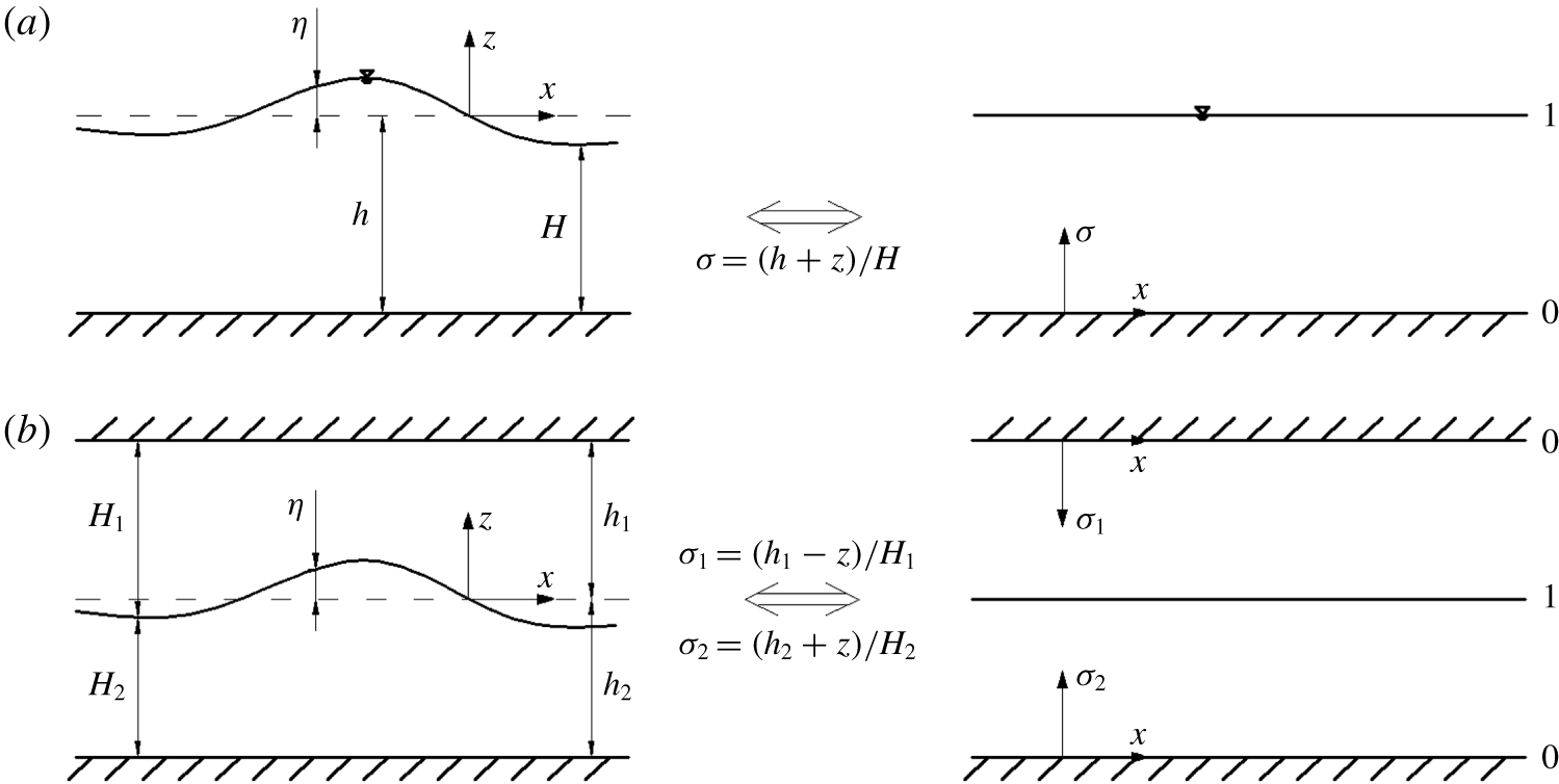
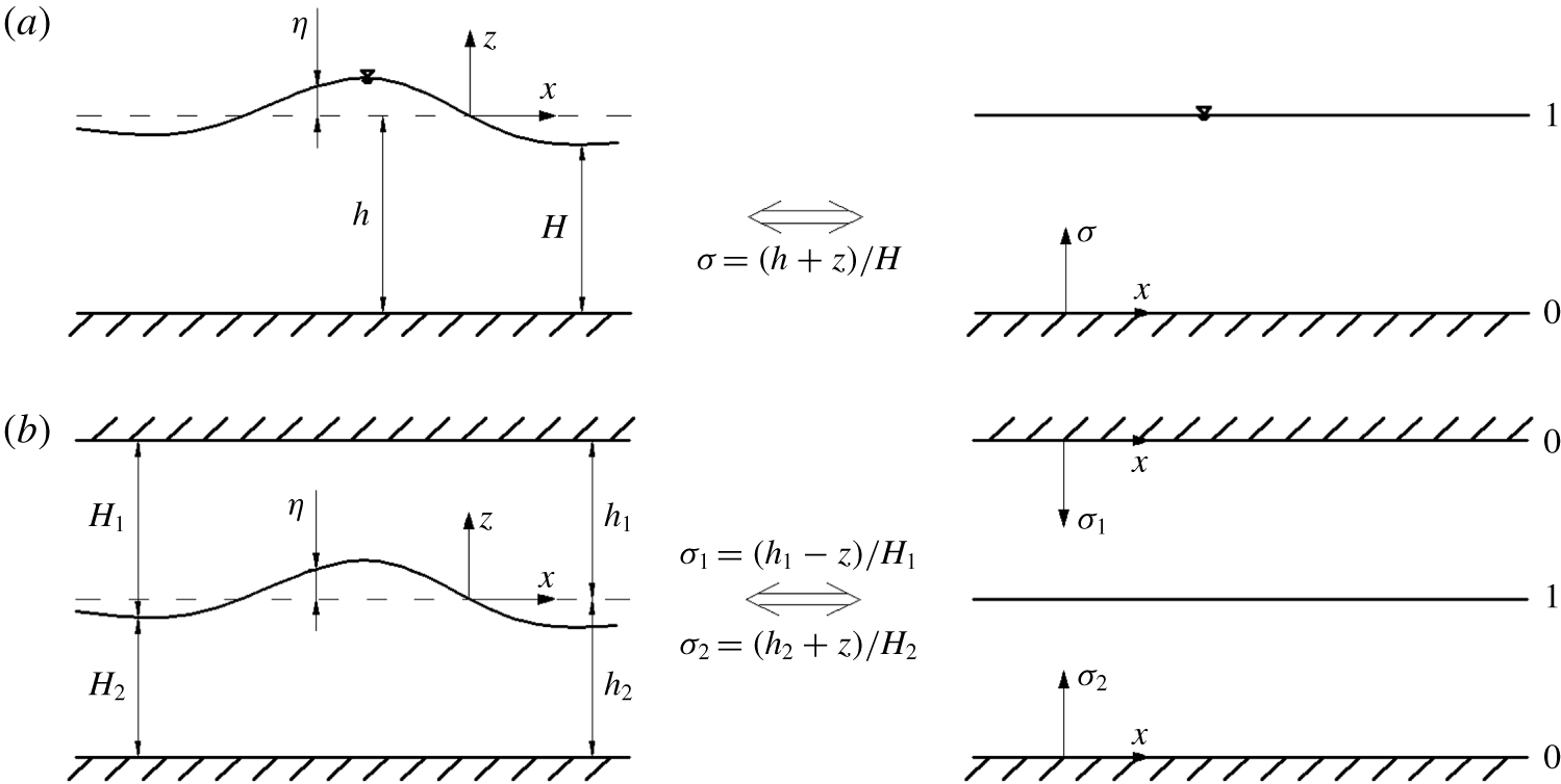
Definition sketch for coordinate systems for (left) Cartesian and (right)  $\unicode[STIX]{x1D70E}$ coordinates for (a) the free-surface problem and (b) the two-layer rigid-lid problem.
2 Governing equations
We consider the irrotational, inviscid motion of an incompressible fluid in a layer of water between a rigid bottom at  $z=-h$ (with
 $h$ constant) and a single-valued surface
 $\unicode[STIX]{x1D702}(\boldsymbol{x}^{\prime },t^{\prime })$ with
 $\boldsymbol{x}^{\prime }=(x^{\prime },y^{\prime })$ indicating horizontal position (figure 1a). We first transform the usual equations for velocity potential
 $\unicode[STIX]{x1D719}$ and surface displacement
 $\unicode[STIX]{x1D702}$ in Cartesian coordinates
 $\boldsymbol{x}^{\prime },z^{\prime },t^{\prime }$ into coordinates
 $\boldsymbol{x},\unicode[STIX]{x1D70E},t$ according to
 $$\begin{eqnarray}\left(\begin{array}{@{}c@{}}\boldsymbol{x}^{\prime }\\ z^{\prime }\\ t^{\prime }\end{array}\right)\rightarrow \left(\begin{array}{@{}c@{}}\boldsymbol{x}=\boldsymbol{x}^{\prime }\\ \unicode[STIX]{x1D70E}=(h+z^{\prime })/H\\ t=t^{\prime }\end{array}\right),\end{eqnarray}$$
where  $H=h+\unicode[STIX]{x1D702}$ is the local total water depth. The transformation maps the physical domain
 $-h\leqslant z^{\prime }\leqslant \unicode[STIX]{x1D702}$ into the constant interval
 $0\leqslant \unicode[STIX]{x1D70E}\leqslant 1$, with
 $\unicode[STIX]{x1D70E}=1$ corresponding to the position of the free surface. We further use standard long wave scaling (
 $\boldsymbol{x}^{\prime }=k_{0}\boldsymbol{x},t^{\prime }=k_{0}c_{0}t,\unicode[STIX]{x1D702}^{\prime }=\unicode[STIX]{x1D702}/a_{0},\unicode[STIX]{x1D719}^{\prime }=(k_{0}h/a_{0}c_{0})\unicode[STIX]{x1D719}$, with
 $c_{0}=\sqrt{gh_{0}}$) where primes now denote dimensionless quantities. Total depth
 $H$ is scaled by the constant
 $h$ to give
 $H^{\prime }=1+\unicode[STIX]{x1D6FF}\unicode[STIX]{x1D702}^{\prime }$, where
 $\unicode[STIX]{x1D6FF}=a_{0}/h$ is the parameter quantifying nonlinearity. Non-dimensionalizing the governing equations leads finally to the dimensionless boundary value problem (with primes now dropped):
 $$\begin{eqnarray}\displaystyle & \displaystyle \unicode[STIX]{x1D707}^{2}(\unicode[STIX]{x1D6FB}^{2}\unicode[STIX]{x1D719}+2\unicode[STIX]{x1D735}\unicode[STIX]{x1D719}_{,\unicode[STIX]{x1D70E}}\boldsymbol{\cdot }\unicode[STIX]{x1D735}\unicode[STIX]{x1D70E}+\unicode[STIX]{x1D6FE}_{2}\unicode[STIX]{x1D719}_{,\unicode[STIX]{x1D70E}})+\unicode[STIX]{x1D6FE}_{1}\unicode[STIX]{x1D719}_{,\unicode[STIX]{x1D70E}\unicode[STIX]{x1D70E}}=0;\quad 0\leqslant \unicode[STIX]{x1D70E}\leqslant 1, & \displaystyle\end{eqnarray}$$
 $$\begin{eqnarray}\displaystyle & \displaystyle \unicode[STIX]{x1D719}_{,\unicode[STIX]{x1D70E}}=0;\quad \unicode[STIX]{x1D70E}=0, & \displaystyle\end{eqnarray}$$
 $$\begin{eqnarray}\displaystyle & \displaystyle (1+\unicode[STIX]{x1D6FF}^{2}\unicode[STIX]{x1D707}^{2}|\unicode[STIX]{x1D735}\unicode[STIX]{x1D702}|^{2})\unicode[STIX]{x1D719}_{,\unicode[STIX]{x1D70E}}=\unicode[STIX]{x1D707}^{2}H(\unicode[STIX]{x1D702}_{,t}+\unicode[STIX]{x1D6FF}\unicode[STIX]{x1D735}\unicode[STIX]{x1D719}\boldsymbol{\cdot }\unicode[STIX]{x1D735}\unicode[STIX]{x1D702});\quad \unicode[STIX]{x1D70E}=1, & \displaystyle\end{eqnarray}$$
 $$\begin{eqnarray}\displaystyle & \displaystyle \unicode[STIX]{x1D707}^{2}\left(\unicode[STIX]{x1D702}+\unicode[STIX]{x1D719}_{,t}+\frac{\unicode[STIX]{x1D6FF}}{2}\unicode[STIX]{x1D735}\unicode[STIX]{x1D719}\boldsymbol{\cdot }\unicode[STIX]{x1D735}\unicode[STIX]{x1D719}\right)-\frac{\unicode[STIX]{x1D6FF}}{2H^{2}}(1+\unicode[STIX]{x1D6FF}^{2}\unicode[STIX]{x1D707}^{2}|\unicode[STIX]{x1D735}\unicode[STIX]{x1D702}|^{2})(\unicode[STIX]{x1D719}_{,\unicode[STIX]{x1D70E}})^{2}=0;\quad \unicode[STIX]{x1D70E}=1, & \displaystyle\end{eqnarray}$$
where  $\unicode[STIX]{x1D707}=k_{0}h$ is the dispersion parameter, subscripted commas denote partial derivatives and where
 $\unicode[STIX]{x1D735}$ denotes a gradient operator in
 $\boldsymbol{x}=(x,y)$. Derivatives of
 $\unicode[STIX]{x1D70E}$ appearing or used in the derivation of (2.2)–(2.5) are given by
 $$\begin{eqnarray}\unicode[STIX]{x1D735}\unicode[STIX]{x1D70E}=-\frac{\unicode[STIX]{x1D707}\unicode[STIX]{x1D70E}}{H}\unicode[STIX]{x1D735}H=-\frac{\unicode[STIX]{x1D707}\unicode[STIX]{x1D70E}}{H}\unicode[STIX]{x1D6FF}\unicode[STIX]{x1D735}\unicode[STIX]{x1D702};\quad \unicode[STIX]{x1D70E}_{,t}=-\frac{\unicode[STIX]{x1D707}\unicode[STIX]{x1D70E}}{H}H_{,t}=-\frac{\unicode[STIX]{x1D707}\unicode[STIX]{x1D70E}}{H}\unicode[STIX]{x1D6FF}\unicode[STIX]{x1D702}_{,t};\quad \unicode[STIX]{x1D70E}_{,z}=H^{-1}.\end{eqnarray}$$
Additional coefficients in (2.2) are given by
 $$\begin{eqnarray}\displaystyle & \displaystyle \unicode[STIX]{x1D6FE}_{1}=|\unicode[STIX]{x1D735}\unicode[STIX]{x1D70E}|^{2}+(\unicode[STIX]{x1D70E}_{,z})^{2}=H^{-2}(1+\unicode[STIX]{x1D707}^{2}\unicode[STIX]{x1D6FF}^{2}\unicode[STIX]{x1D70E}^{2}|\unicode[STIX]{x1D735}\unicode[STIX]{x1D702}|^{2}), & \displaystyle\end{eqnarray}$$
 $$\begin{eqnarray}\displaystyle & \displaystyle \unicode[STIX]{x1D6FE}_{2}=\unicode[STIX]{x1D6FB}^{2}\unicode[STIX]{x1D70E}+\unicode[STIX]{x1D735}\unicode[STIX]{x1D70E}\boldsymbol{\cdot }(\unicode[STIX]{x1D735}\unicode[STIX]{x1D70E})_{,\unicode[STIX]{x1D70E}}=(3\unicode[STIX]{x1D6FF}^{2}H^{-2}|\unicode[STIX]{x1D735}\unicode[STIX]{x1D702}|^{2}-\unicode[STIX]{x1D6FF}H^{-1}\unicode[STIX]{x1D6FB}^{2}\unicode[STIX]{x1D702})\unicode[STIX]{x1D70E}. & \displaystyle\end{eqnarray}$$
The set of surface boundary conditions (2.4)–(2.5) take on a form consistent with the canonical equations of (Zakharov Reference Zakharov1968) with vertical velocity  $W$ given by
 $\unicode[STIX]{x1D719}_{,\unicode[STIX]{x1D70E}}/H$, but with a more complex problem (2.2)–(2.3) for the internal flow field. (We note that
 $\unicode[STIX]{x1D719}_{,\unicode[STIX]{x1D70E}}$ is oriented normal to the surface, rather than in the vertical). Finally, it is advantageous in deriving the models below to have a conservation law for volume. This is obtained by integrating (2.2) over depth and using (2.3) and (2.4) to obtain
 $$\begin{eqnarray}\unicode[STIX]{x1D702}_{,t}+\unicode[STIX]{x1D735}\boldsymbol{\cdot }\boldsymbol{Q}=0;\quad \boldsymbol{Q}=H\int _{0}^{1}\unicode[STIX]{x1D735}\unicode[STIX]{x1D719}\,\text{d}\unicode[STIX]{x1D70E}-\unicode[STIX]{x1D735}\unicode[STIX]{x1D702}\int _{0}^{1}\unicode[STIX]{x1D70E}\unicode[STIX]{x1D719}_{,\unicode[STIX]{x1D70E}}\,\text{d}\unicode[STIX]{x1D70E}.\end{eqnarray}$$
3 Boussinesq equations
We next use the equations from the previous section to obtain two variants of Boussinesq equations truncated to leading order  $O(\unicode[STIX]{x1D707}^{2})$, corresponding, for example, to the weakly dispersive equations in weakly nonlinear (Peregrine Reference Peregrine1966; Nwogu Reference Nwogu1993) or fully nonlinear (Serre Reference Serre1953; Su & Gardner Reference Su and Gardner1969; Wei et al. Reference Wei, Kirby, Grilli and Subramanya1995) form.
3.1 Model 1: expansion about  $\unicode[STIX]{x1D70E}=0$

The first model considered is based on an expansion about the position of the bottom at  $\unicode[STIX]{x1D70E}=0$, leading to the expression
 $$\begin{eqnarray}\unicode[STIX]{x1D719}(\boldsymbol{x},\unicode[STIX]{x1D70E},t)=\mathop{\sum }_{n=0}^{\infty }\unicode[STIX]{x1D719}_{n}(\boldsymbol{x},t)\unicode[STIX]{x1D70E}(\boldsymbol{x},t)^{n}.\end{eqnarray}$$
The bottom boundary condition (2.3) immediately gives  $\unicode[STIX]{x1D719}_{1}=0$. Laplace’s equation (2.2) then gives the leading order result
 $$\begin{eqnarray}\unicode[STIX]{x1D719}_{2}=-\unicode[STIX]{x1D707}^{2}\frac{H^{2}}{2}\unicode[STIX]{x1D6FB}^{2}\unicode[STIX]{x1D719}_{0}=-\unicode[STIX]{x1D707}^{2}\frac{H^{2}}{2}\unicode[STIX]{x1D735}\boldsymbol{\cdot }\boldsymbol{u}_{0},\end{eqnarray}$$
where  $\boldsymbol{u}_{0}=\unicode[STIX]{x1D735}\unicode[STIX]{x1D719}_{0}$ is identified as being the horizontal velocity at the bottom,
 $\unicode[STIX]{x1D70E}=0$. Using these results in (2.9) gives the first of two equations for
 $\unicode[STIX]{x1D702}$ and
 $\boldsymbol{u}_{0}$:
 $$\begin{eqnarray}\unicode[STIX]{x1D702}_{,t}+\unicode[STIX]{x1D735}\boldsymbol{\cdot }\left\{H\boldsymbol{u}_{0}+\frac{\unicode[STIX]{x1D707}^{2}}{6}[2A\unicode[STIX]{x1D735}H-H\unicode[STIX]{x1D735}A]\right\}=O(\unicode[STIX]{x1D707}^{4});\quad A=H^{2}\unicode[STIX]{x1D735}\boldsymbol{\cdot }\boldsymbol{u}_{0}.\end{eqnarray}$$
The second equation follows from taking the gradient of the dynamic surface boundary condition (2.5) and retaining terms to  $O(\unicode[STIX]{x1D707}^{2})$ to get
 $$\begin{eqnarray}\boldsymbol{u}_{0,t}+\unicode[STIX]{x1D6FF}\boldsymbol{u}_{0}\boldsymbol{\cdot }\unicode[STIX]{x1D735}\boldsymbol{u}_{0}+\unicode[STIX]{x1D735}\unicode[STIX]{x1D702}-\frac{\unicode[STIX]{x1D707}^{2}}{2}\unicode[STIX]{x1D735}(A_{,t}+\unicode[STIX]{x1D6FF}\boldsymbol{u}_{0}\boldsymbol{\cdot }\unicode[STIX]{x1D735}A)-\frac{3}{2}\unicode[STIX]{x1D6FF}\unicode[STIX]{x1D707}^{2}\unicode[STIX]{x1D735}(H^{-2}A^{2})=O(\unicode[STIX]{x1D707}^{4}).\end{eqnarray}$$
The model (3.3)–(3.4) may be linearized in order to determine the corresponding linear dispersion relation
 $$\begin{eqnarray}\unicode[STIX]{x1D714}^{2}=k^{2}\frac{1+\frac{1}{6}\unicode[STIX]{x1D707}^{2}k^{2}}{1+\frac{1}{2}\unicode[STIX]{x1D707}^{2}k^{2}},\end{eqnarray}$$
where  $\unicode[STIX]{x1D714}$ and
 $k$ are dimensionless frequency and wavenumber of component linear waves. The resulting model is a legitimate leading-order Boussinesq model, in that the dispersion relation is asymptotically equivalent to the leading-order Taylor series expansion
 $\unicode[STIX]{x1D714}^{2}=k\tanh \unicode[STIX]{x1D707}k=k^{2}(1-\frac{1}{3}\unicode[STIX]{x1D707}^{2}k^{2}+O(\unicode[STIX]{x1D707}^{4}))$, but is not in an optimal form for a model of this type. This adjustment is considered next.
3.2 Model 2: expansion about an arbitrary level $\unicode[STIX]{x1D70E}_{\unicode[STIX]{x1D6FC}}$

The goal in optimizing an  $O(\unicode[STIX]{x1D707}^{2})$ model is to obtain a dispersion relation corresponding to the (2,2) Padé expression (Nwogu Reference Nwogu1993)
 $$\begin{eqnarray}\unicode[STIX]{x1D714}^{2}=k^{2}\frac{1+\frac{1}{15}\unicode[STIX]{x1D707}^{2}k^{2}}{1+\frac{2}{5}\unicode[STIX]{x1D707}^{2}k^{2}}.\end{eqnarray}$$
To this end, we consider the alternate expansion
 $$\begin{eqnarray}\unicode[STIX]{x1D719}=\mathop{\sum }_{n=0}^{\infty }\tilde{\unicode[STIX]{x1D719}}_{n}(\unicode[STIX]{x1D70E}-\unicode[STIX]{x1D70E}_{\unicode[STIX]{x1D6FC}})^{n}.\end{eqnarray}$$
Evaluating (3.7) and (3.1) at  $\unicode[STIX]{x1D70E}_{\unicode[STIX]{x1D6FC}}$ and comparing results gives
 $$\begin{eqnarray}\tilde{\unicode[STIX]{x1D719}}_{0}=\unicode[STIX]{x1D719}_{0}+\unicode[STIX]{x1D719}_{2}\unicode[STIX]{x1D70E}_{\unicode[STIX]{x1D6FC}}^{2}+O(\unicode[STIX]{x1D707}^{4}).\end{eqnarray}$$
Taking the gradient of (3.8) and rearranging gives
 $$\begin{eqnarray}\boldsymbol{u}_{0}=\boldsymbol{u}_{\unicode[STIX]{x1D6FC}}+\frac{\unicode[STIX]{x1D707}^{2}}{6}\unicode[STIX]{x1D70E}_{\unicode[STIX]{x1D6FC}}^{2}\unicode[STIX]{x1D735}A^{\prime }+O(\unicode[STIX]{x1D707}^{4});\quad A^{\prime }=H^{2}\unicode[STIX]{x1D735}\boldsymbol{\cdot }\boldsymbol{u}_{\unicode[STIX]{x1D6FC}},\end{eqnarray}$$
where  $\boldsymbol{u}_{\unicode[STIX]{x1D6FC}}=\unicode[STIX]{x1D735}\tilde{\unicode[STIX]{x1D719}}_{0}$. Using (3.9) directly in the model (3.3)–(3.4) gives the revised system
 $$\begin{eqnarray}\unicode[STIX]{x1D702}_{,t}+\unicode[STIX]{x1D735}\boldsymbol{\cdot }\left[H\boldsymbol{u}_{\unicode[STIX]{x1D6FC}}+\frac{\unicode[STIX]{x1D707}^{2}}{2}\left(\unicode[STIX]{x1D70E}_{\unicode[STIX]{x1D6FC}}^{2}-\frac{1}{3}\right)H\unicode[STIX]{x1D735}A^{\prime }+\frac{\unicode[STIX]{x1D707}^{2}}{3}A^{\prime }\unicode[STIX]{x1D735}H\right]=O(\unicode[STIX]{x1D707}^{4}),\end{eqnarray}$$
 $$\begin{eqnarray}\displaystyle & & \displaystyle \boldsymbol{u}_{\unicode[STIX]{x1D6FC},t}+\unicode[STIX]{x1D6FF}\boldsymbol{u}_{\unicode[STIX]{x1D6FC}}\boldsymbol{\cdot }\unicode[STIX]{x1D735}\boldsymbol{u}_{\unicode[STIX]{x1D6FC}}+\unicode[STIX]{x1D735}\unicode[STIX]{x1D702}+\frac{\unicode[STIX]{x1D707}^{2}}{2}(\unicode[STIX]{x1D70E}_{\unicode[STIX]{x1D6FC}}^{2}-1)\unicode[STIX]{x1D735}(A_{,t}^{\prime }+\unicode[STIX]{x1D6FF}\boldsymbol{u}_{\unicode[STIX]{x1D6FC}}\boldsymbol{\cdot }\unicode[STIX]{x1D735}A^{\prime })\nonumber\\ \displaystyle & & \displaystyle \quad -\,\frac{3}{2}\unicode[STIX]{x1D6FF}\unicode[STIX]{x1D707}^{2}\unicode[STIX]{x1D735}(H^{2}(\unicode[STIX]{x1D735}\boldsymbol{\cdot }\boldsymbol{u}_{\unicode[STIX]{x1D6FC}})^{2})=O(\unicode[STIX]{x1D707}^{4}).\end{eqnarray}$$
The revised system can be compared to the fully nonlinear Boussinesq model of Wei et al. (Reference Wei, Kirby, Grilli and Subramanya1995), and will be examined for trough instabilities in the following section. The linearized form has the dimensional dispersion relation
 $$\begin{eqnarray}\unicode[STIX]{x1D714}^{2}=gk^{2}hP(kh);\quad P(kh)=\frac{1-\frac{1}{2}(\unicode[STIX]{x1D70E}_{\unicode[STIX]{x1D6FC}}^{2}-\frac{1}{3})(kh)^{2}}{1-\frac{1}{2}(\unicode[STIX]{x1D70E}_{\unicode[STIX]{x1D6FC}}^{2}-1)(kh)^{2}},\end{eqnarray}$$
where the choice  $\unicode[STIX]{x1D70E}_{\unicode[STIX]{x1D6FC}}=0$ recovers the results of the previous section, while the choice
 $\unicode[STIX]{x1D70E}_{\unicode[STIX]{x1D6FC}}=1/\sqrt{5}$ recovers the Padé form (3.6) and is thus considered optimal in the sense mentioned above. The model (3.10)–(3.11) is closely related to the particular case of
 $z_{\unicode[STIX]{x1D6FC}}=-h+\unicode[STIX]{x1D70E}_{\unicode[STIX]{x1D6FC}}H$ in KKCD01 equation (17), which places
 $z_{\unicode[STIX]{x1D6FC}}$ at the fixed elevation
 $\unicode[STIX]{x1D70E}_{\unicode[STIX]{x1D6FC}}$ and differs from the present model only in the definition of the dependent variable
 $\boldsymbol{u}_{\unicode[STIX]{x1D6FC}}$, discussed in § 6. We examine the present equations in the following section but remark that the results are the same for the earlier model.
4 Stability properties near long wave troughs
As mentioned by Reference Madsen and FuhrmanMF20, the Boussinesq model of Wei et al. (Reference Wei, Kirby, Grilli and Subramanya1995) is subject to a possible short wave instability concentrated in the trough region of long wave disturbances. Modern versions of the codes based on this model (Shi et al. Reference Shi, Kirby, Harris, Geiman and Grilli2012) are based on variations of the original model which correct for effects of vertical vorticity (Chen Reference Chen2006), and which allow for vertical motion of the reference level for Taylor expansions in response to surface motion (KKCD01). The first correction drops out in a one-dimensional horizontal analysis. However, as mentioned above, the second modification allows for a special case that brings the earlier model in line with the discussion here. We review the analysis for the Wei et al. (Reference Wei, Kirby, Grilli and Subramanya1995) model using a version reduced to constant depth and one horizontal direction, as in Reference Madsen and FuhrmanMF20, and then consider the model of § 3.2.
4.1 Model of Wei et al. (Reference Wei, Kirby, Grilli and Subramanya1995)
The FNBTE of Wei et al. (Reference Wei, Kirby, Grilli and Subramanya1995), reduced to constant depth and one horizontal dimension, may be written (in dimensional form) as
 $$\begin{eqnarray}\displaystyle & \displaystyle \unicode[STIX]{x1D702}_{,t}+(Hu)_{,x}+(\unicode[STIX]{x1D6FC}+{\textstyle \frac{1}{3}})h^{3}u_{,xxx}+\unicode[STIX]{x1D6EC}_{1}=0, & \displaystyle\end{eqnarray}$$
 $$\begin{eqnarray}\displaystyle & \displaystyle u_{,t}+uu_{,x}+g\unicode[STIX]{x1D702}_{,x}+\unicode[STIX]{x1D6FC}h^{2}u_{,xxt}+\unicode[STIX]{x1D6EC}_{2}=0, & \displaystyle\end{eqnarray}$$
with nonlinear dispersive terms  $\unicode[STIX]{x1D6EC}_{1}$ and
 $\unicode[STIX]{x1D6EC}_{2}$ given by
 $$\begin{eqnarray}\displaystyle & \displaystyle \unicode[STIX]{x1D6EC}_{1}=[(\unicode[STIX]{x1D6FC}h^{2}\unicode[STIX]{x1D702}-{\textstyle \frac{1}{2}}h\unicode[STIX]{x1D702}^{2}-{\textstyle \frac{1}{6}}\unicode[STIX]{x1D702}^{3})u_{,xx}]_{,x}, & \displaystyle\end{eqnarray}$$
 $$\begin{eqnarray}\displaystyle & \displaystyle \unicode[STIX]{x1D6EC}_{2}=[(\unicode[STIX]{x1D6FC}h^{2}-h\unicode[STIX]{x1D702}-{\textstyle \frac{1}{2}}\unicode[STIX]{x1D702}^{2})uu_{,xx}-(h\unicode[STIX]{x1D702}+{\textstyle \frac{1}{2}}\unicode[STIX]{x1D702}^{2})u_{,xt}+{\textstyle \frac{1}{2}}H^{2}(u_{,x})^{2}]_{,x}, & \displaystyle\end{eqnarray}$$
where  $\unicode[STIX]{x1D6FC}=(z_{\unicode[STIX]{x1D6FC}}/h)^{2}/2+z_{\unicode[STIX]{x1D6FC}}/h$ and
 $z_{\unicode[STIX]{x1D6FC}}$ is the reference elevation for Taylor expansions in
 $z$. The choice
 $\unicode[STIX]{x1D6FC}=-2/5$ recovers the (2,2) Padé expression (3.6) for the linear dispersion relation.
The analysis proceeds by taking  $(\overline{\unicode[STIX]{x1D702}},\overline{u})$ to be a solution of (4.1)–(4.2) and then introducing perturbations
 $(\tilde{\unicode[STIX]{x1D702}},\tilde{u} )$. Substituting
 $\unicode[STIX]{x1D702}=\overline{\unicode[STIX]{x1D702}}+\tilde{\unicode[STIX]{x1D702}},u=\overline{u}+\tilde{u}$ in (4.1)–(4.2), eliminating the equation for
 $(\overline{\unicode[STIX]{x1D702}},\overline{u})$ alone, and linearizing the remaining equations for the perturbations leads to a coupled set of equations for
 $(\tilde{\unicode[STIX]{x1D702}},\tilde{u} )$ with associated dispersion relation
 $$\begin{eqnarray}\tilde{\unicode[STIX]{x1D714}}^{2}=(\unicode[STIX]{x1D714}-k\overline{u})^{2}=gk^{2}\overline{H}\hat{P}(k\overline{H},\unicode[STIX]{x1D6FE}),\end{eqnarray}$$
where  $\overline{H}=h+\overline{\unicode[STIX]{x1D702}}$ and
 $$\begin{eqnarray}\hat{P}=\frac{\displaystyle 1-\left(\unicode[STIX]{x1D6FC}+\frac{1}{3}-\frac{\unicode[STIX]{x1D6FE}}{6}\right)(k\overline{H})^{2}}{\displaystyle 1-\left(\unicode[STIX]{x1D6FC}-\frac{\unicode[STIX]{x1D6FE}}{2}\right)(k\overline{H})^{2}},\end{eqnarray}$$
with  $\unicode[STIX]{x1D6FE}=(\overline{\unicode[STIX]{x1D702}}/h)(2+\overline{\unicode[STIX]{x1D702}}/h)$. Instability results when the numerator and denominator of
 $\hat{P}$ are of opposite sign. As described in Reference Madsen and FuhrmanMF20 and shown in their figure 14, the unstable region is bounded above by the locus of the zero in the numerator, given by
 $$\begin{eqnarray}\unicode[STIX]{x1D6FE}=-\frac{2}{5}-\frac{6}{(kh)^{2}}\end{eqnarray}$$
and below by the zero in the denominator, given by
 $$\begin{eqnarray}\unicode[STIX]{x1D6FE}=-\frac{4}{5}-\frac{1}{(kh)^{2}}.\end{eqnarray}$$
Both curves converge at the point  $\unicode[STIX]{x1D6FE}=\overline{\unicode[STIX]{x1D702}}/h=-1,kh=\sqrt{10}$, with the model being stable for
 $kh<\sqrt{10}$.
4.2 The model of § 3.2
Rewriting the model of § 3.2 in one horizontal dimension and in dimensional form gives the equations
 $$\begin{eqnarray}\displaystyle & \displaystyle \unicode[STIX]{x1D702}_{t}+[Hu+{\textstyle \frac{1}{2}}(\unicode[STIX]{x1D70E}_{\unicode[STIX]{x1D6FC}}^{2}-{\textstyle \frac{1}{3}})H(H^{2}u_{,x})_{,x}+{\textstyle \frac{1}{3}}H^{2}H_{,x}u_{,x}]_{,x}=0, & \displaystyle\end{eqnarray}$$
 $$\begin{eqnarray}\displaystyle & \displaystyle u_{,t}+uu_{,x}+g\unicode[STIX]{x1D702}_{,x}+{\textstyle \frac{1}{2}}(\unicode[STIX]{x1D70E}_{\unicode[STIX]{x1D6FC}}^{2}-1)[(H^{2}u_{,x})_{,t}+u(H^{2}u_{,x})_{,x}]_{,x}-{\textstyle \frac{3}{2}}[H^{2}(u_{,x})^{2}]_{,x}=0. & \displaystyle\end{eqnarray}$$
Applying the same procedure as in the previous example leads to a linearized system for the perturbation with dispersion relation
 $$\begin{eqnarray}\tilde{\unicode[STIX]{x1D714}}^{2}=(\unicode[STIX]{x1D714}-k\overline{u})^{2}=gk^{2}\overline{H}P(k\overline{H}),\end{eqnarray}$$
where  $P$ is defined in (3.12). Aside from a shift in water depth from
 $h$ to
 $\overline{H}$ and the added effect of advection by the mean flow
 $\overline{u}$, (4.11) is identical to the original dispersion relation (3.12) for the linear version of the full Boussinesq model. Solving (4.11) for frequency
 $\unicode[STIX]{x1D714}$ gives
 $$\begin{eqnarray}\unicode[STIX]{x1D714}=k(\overline{u}\pm (g\overline{H}P)^{1/2}).\end{eqnarray}$$
Given that  $\overline{H}>0$, the condition for stability of the perturbed system is the same as the condition for stability of the original linearized system, which is guaranteed for all
 $kh$ if
 $\unicode[STIX]{x1D70E}_{\unicode[STIX]{x1D6FC}}^{2}<1/3$. A properly configured, linearly stable implementation of the model (3.10)–(3.11) is thus stable in the nonlinear sense examined by Reference Madsen and FuhrmanMF20.
5 An example for internal waves in a two-layer system
Here, we illustrate the application of the  $\unicode[STIX]{x1D70E}$ coordinate transformation in the derivation of a FNBTE with enhanced dispersion for internal waves in a two-layer system (figure 1b).
5.1 The model of Choi & Camassa (Reference Choi and Camassa1999)
We first examine the FNBTE model of Choi & Camassa (Reference Choi and Camassa1999) for internal waves in a shallow two-layer system with fixed upper boundary. The layer properties are undisturbed depths  $h_{i}$ and fluid densities
 $\unicode[STIX]{x1D70C}_{i};i=1,2$ for the upper and lower layers, with
 $\unicode[STIX]{x1D70C}_{1}\leqslant \unicode[STIX]{x1D70C}_{2}$. We denote the interface displacement as
 $\unicode[STIX]{x1D702}(x,t)$ and define the total layer depths as
 $H_{1}=h_{1}-\unicode[STIX]{x1D702}$ and
 $H_{2}=h_{2}+\unicode[STIX]{x1D702}$. The model of Choi & Camassa (Reference Choi and Camassa1999) is then given in terms of layer-averaged horizontal velocities by
 $$\begin{eqnarray}\displaystyle & \displaystyle \unicode[STIX]{x1D702}_{,t}+(H_{2}u_{2})_{,x}=0, & \displaystyle\end{eqnarray}$$
 $$\begin{eqnarray}\displaystyle & \displaystyle R\left[u_{1,t}+u_{1}u_{1,x}-\frac{1}{3H_{1}}(H_{1}^{3}G_{1})_{,x}\right]=\left[u_{2,t}+u_{2}u_{2,x}-\frac{1}{3H_{2}}(H_{2}^{3}G_{2})_{,x}\right]+g^{\prime }\unicode[STIX]{x1D702}_{x}, & \displaystyle\end{eqnarray}$$
where we invoke the assumption of no motion at infinity to close the system according to
 $$\begin{eqnarray}u_{1}=-\unicode[STIX]{x1D6FE}u_{2};\quad \unicode[STIX]{x1D6FE}=H_{2}/H_{1}\end{eqnarray}$$
and where  $R=\unicode[STIX]{x1D70C}_{1}/\unicode[STIX]{x1D70C}_{2}\leqslant 1$,
 $g^{\prime }=(1-R)g$ is reduced gravity, and
 $$\begin{eqnarray}G_{i}=u_{i,xt}+u_{i}u_{i,xx}-(u_{i,x})^{2}.\end{eqnarray}$$
The linearized version of (5.1)–(5.2) has the dispersion relation
 $$\begin{eqnarray}\unicode[STIX]{x1D714}^{2}=\frac{g^{\prime }k^{2}h_{1}h_{2}}{h_{1}/\tilde{P}_{2}+Rh_{2}/\tilde{P}_{1}};\quad \tilde{P}_{i}=\tilde{P}(kh_{i}),\end{eqnarray}$$
which is consistent with unenhanced one-layer models based on depth-average velocity, such as the BTE of Peregrine (Reference Peregrine1966) or the FNBTE of Serre (Reference Serre1953).
Turning to the nonlinear stability analysis, we first note that the interpretation of results is complicated by the fact that the resulting system describes perturbations propagating on an interface with non-zero vorticity. This configuration is always unstable to sufficiently short perturbations even when full linear dispersion is considered, as long as surface tension is neglected (Liska, Margolin & Wendroff Reference Liska, Margolin and Wendroff1995). This region of instability overlaps the short wave instability being considered. Applying the analysis of Reference Madsen and FuhrmanMF20 leads to the dispersion relation
 $$\begin{eqnarray}(R\overline{H}_{2}/\tilde{P}(k\overline{H}_{1}))\tilde{\unicode[STIX]{x1D714}}_{1}^{2}+(\overline{H}_{1}/\tilde{P}(k\overline{H}_{2}))\tilde{\unicode[STIX]{x1D714}}_{2}^{2}=g^{\prime }k^{2}\overline{H}_{1}\overline{H}_{2},\end{eqnarray}$$
where intrinsic frequencies for each layer are given by  $\tilde{\unicode[STIX]{x1D714}}_{i}=\unicode[STIX]{x1D714}-k\overline{u}_{i}$. The correspondence between (5.5) and (5.6) is apparent and, in the absence of interfacial shear, would lead to the conclusion that the resulting system is stable in the sense of Reference Madsen and FuhrmanMF20. However, solving the quadratic equation (5.6) for
 $\unicode[STIX]{x1D714}$ and requiring that its discriminant be positive leads to the condition
 $$\begin{eqnarray}\tilde{\unicode[STIX]{x1D6E5}}=g^{\prime }[R\overline{H}_{2}\tilde{P}(k\overline{H}_{2})+\overline{H}_{1}\tilde{P}(k\overline{H}_{1})]/R>(\overline{u}_{1}-\overline{u}_{2})^{2}.\end{eqnarray}$$
Since  $\tilde{P}\sim k^{-2}$ for sufficiently large
 $k$, the stability condition (5.7) will fail for sufficiently strong shear or short wavelength perturbations.
5.2 A dispersion-enhanced model in $\unicode[STIX]{x1D70E}$ coordinates

We now follow § 3 and develop an enhanced version of the model of Choi & Camassa (Reference Choi and Camassa1999) aimed at recovering a more accurate form of the corresponding linear dispersion relation. As was the case with the free-surface model of KKCD01, the present derivation mirrors the previous development of an enhanced model in Cartesian coordinates by Choi, Barros & Jo (Reference Choi, Barros and Jo2009). The derivation proceeds as before with the addition of an upper layer with  $\unicode[STIX]{x1D70E}$ coordinate
 $\unicode[STIX]{x1D70E}_{1}=(h_{1}-z)/H_{1}$, and with lower-layer quantities designated with subscript 2. The domain is defined with the stationary interface at
 $z=0$ and upper and lower boundaries at
 $z=h_{1}$ and
 $z=-h_{2}$. Following the same steps as in § 3.2, we obtain the equations governing volume conservation in each layer,
 $$\begin{eqnarray}\displaystyle & \displaystyle -\unicode[STIX]{x1D702}_{,t}+\unicode[STIX]{x1D735}\boldsymbol{\cdot }\left[H_{1}\boldsymbol{u}_{\unicode[STIX]{x1D6FC}1}+\frac{\unicode[STIX]{x1D707}^{2}}{2}\left(\unicode[STIX]{x1D70E}_{\unicode[STIX]{x1D6FC}}^{2}-\frac{1}{3}\right)H_{1}\unicode[STIX]{x1D735}A_{1}^{\prime }+\frac{\unicode[STIX]{x1D707}^{2}}{3}A_{1}^{\prime }\unicode[STIX]{x1D735}H_{1}\right]=O(\unicode[STIX]{x1D707}^{4}), & \displaystyle\end{eqnarray}$$
 $$\begin{eqnarray}\displaystyle & \displaystyle \unicode[STIX]{x1D702}_{,t}+\unicode[STIX]{x1D735}\boldsymbol{\cdot }\left[H_{2}\boldsymbol{u}_{\unicode[STIX]{x1D6FC}2}+\frac{\unicode[STIX]{x1D707}^{2}}{2}\left(\unicode[STIX]{x1D70E}_{\unicode[STIX]{x1D6FC}}^{2}-\frac{1}{3}\right)H_{2}\unicode[STIX]{x1D735}A_{2}^{\prime }+\frac{\unicode[STIX]{x1D707}^{2}}{3}A_{2}^{\prime }\unicode[STIX]{x1D735}H_{2}\right]=O(\unicode[STIX]{x1D707}^{4}), & \displaystyle\end{eqnarray}$$
while continuity of pressure at the interface gives the relation
 $$\begin{eqnarray}\displaystyle & & \displaystyle R\left[\boldsymbol{u}_{\unicode[STIX]{x1D6FC}1,t}+\unicode[STIX]{x1D6FF}\boldsymbol{u}_{\unicode[STIX]{x1D6FC}1}\boldsymbol{\cdot }\unicode[STIX]{x1D735}\boldsymbol{u}_{\unicode[STIX]{x1D6FC}1}+\unicode[STIX]{x1D735}\unicode[STIX]{x1D702}+\frac{\unicode[STIX]{x1D707}^{2}}{2}(\unicode[STIX]{x1D70E}_{\unicode[STIX]{x1D6FC}}^{2}-1)\unicode[STIX]{x1D735}(A_{1,t}^{\prime }+\unicode[STIX]{x1D6FF}\boldsymbol{u}_{\unicode[STIX]{x1D6FC}1}\boldsymbol{\cdot }\unicode[STIX]{x1D735}A_{1}^{\prime })\right.\nonumber\\ \displaystyle & & \displaystyle \quad -\left.\frac{3}{2}\unicode[STIX]{x1D6FF}\unicode[STIX]{x1D707}^{2}\unicode[STIX]{x1D735}(H_{1}^{-2}(A_{1}^{\prime })^{2})\right]=\left[\boldsymbol{u}_{\unicode[STIX]{x1D6FC}2,t}+\unicode[STIX]{x1D6FF}\boldsymbol{u}_{\unicode[STIX]{x1D6FC}2}\boldsymbol{\cdot }\unicode[STIX]{x1D735}\boldsymbol{u}_{\unicode[STIX]{x1D6FC}2}+\unicode[STIX]{x1D735}\unicode[STIX]{x1D702}\right.\nonumber\\ \displaystyle & & \displaystyle \quad +\left.\frac{\unicode[STIX]{x1D707}^{2}}{2}(\unicode[STIX]{x1D70E}_{\unicode[STIX]{x1D6FC}}^{2}-1)\unicode[STIX]{x1D735}(A_{2,t}^{\prime }+\unicode[STIX]{x1D6FF}\boldsymbol{u}_{\unicode[STIX]{x1D6FC}2}\boldsymbol{\cdot }\unicode[STIX]{x1D735}A_{2}^{\prime })-\frac{3}{2}\unicode[STIX]{x1D6FF}\unicode[STIX]{x1D707}^{2}\unicode[STIX]{x1D735}(H_{2}^{-2}(A_{2}^{\prime })^{2})\right].\end{eqnarray}$$
The linearization of the system leads to the dispersion relation
 $$\begin{eqnarray}\unicode[STIX]{x1D714}^{2}=\frac{g^{\prime }k^{2}h_{1}h_{2}}{Rh_{2}/P_{1}+h_{1}/P_{2}},\end{eqnarray}$$
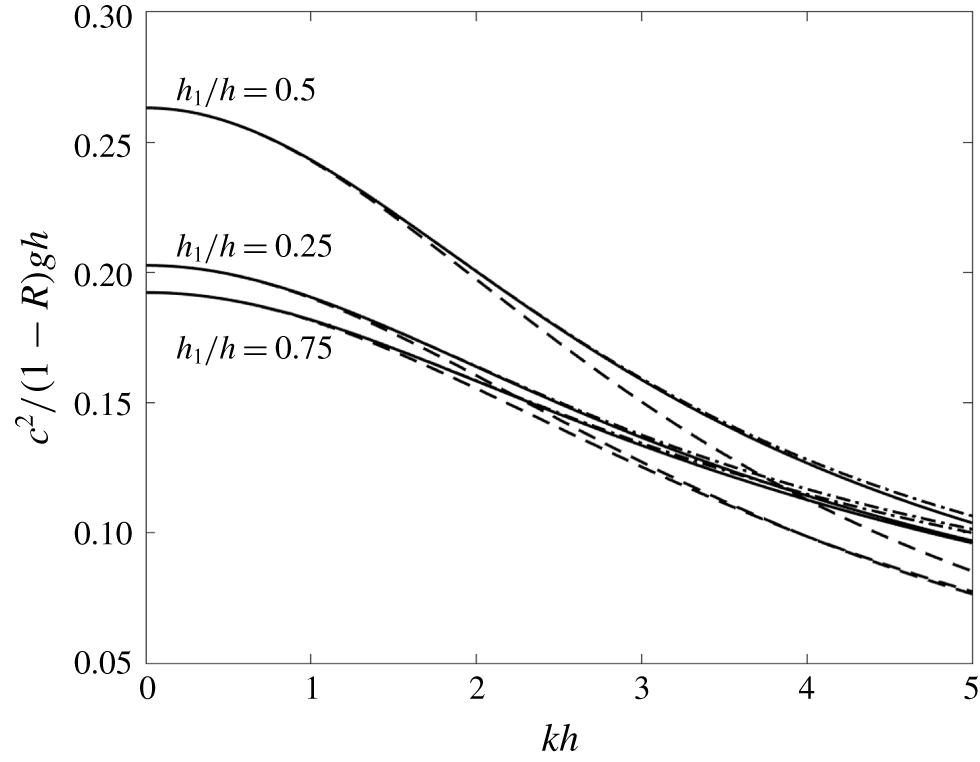
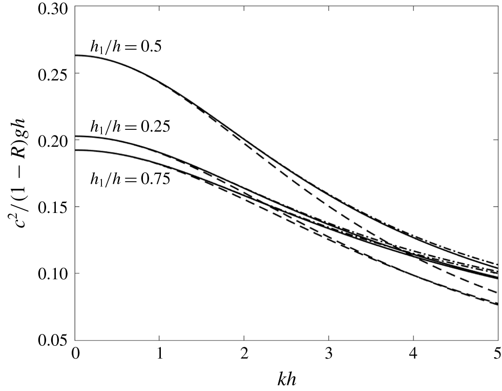
where  $P_{i}=P(kh_{i})$ is defined in (3.12). The phase speed predicted by the Choi & Camassa model and the present enhanced model (5.8)–(5.10) are shown as a function of
 $kh$ in figure 2 for
 $R=0.9$ and three upper-layer thicknesses
 $h_{1}/h=0.25,0.5$ and
 $0.75$, where
 $h=h_{1}+h_{2}$ is the total depth of the channel. Full linear theory results are given by
 $$\begin{eqnarray}\frac{c^{2}}{g^{\prime }h}=\frac{1}{R\coth (kh_{1})+\coth (kh_{2})};c=\unicode[STIX]{x1D714}/k.\end{eqnarray}$$
The enhancement provided by the use of reference level  $\unicode[STIX]{x1D70E}_{\unicode[STIX]{x1D6FC}}$ in each layer is comparable to the improvement achieved in single-layer models for free-surface waves. In deriving and analysing a similar model following an enhancement procedure in Cartesian coordinates (as in Wei et al. (Reference Wei, Kirby, Grilli and Subramanya1995)), Choi et al. (Reference Choi, Barros and Jo2009) point out that it is preferable to use the free choice of parameters to aid in suppressing the shear instability rather than enhancing dispersive properties as the waves in question are rather long. Carrying out the stability analysis as before leads to the revised dispersion relation
 $$\begin{eqnarray}(R\overline{H}_{2}/P(k\overline{H}_{1}))\tilde{\unicode[STIX]{x1D714}}_{1}^{2}+(\overline{H}_{1}/P(k\overline{H}_{2}))\tilde{\unicode[STIX]{x1D714}}_{2}^{2}=g^{\prime }k^{2}\overline{H}_{1}\overline{H}_{2}\end{eqnarray}$$
and stability criterion
 $$\begin{eqnarray}\unicode[STIX]{x1D6E5}=g^{\prime }[R\overline{H}_{2}P(k\overline{H}_{2})+\overline{H}_{1}P(k\overline{H}_{1})]/R>(\overline{u}_{1}-\overline{u}_{2})^{2}.\end{eqnarray}$$
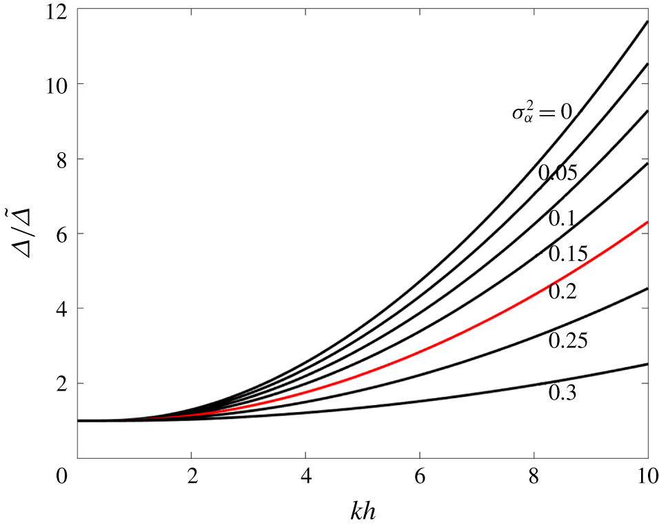
The ratio  $\unicode[STIX]{x1D6E5}/\tilde{\unicode[STIX]{x1D6E5}}$ provides an indication of the enhancement of stability for a given shear, and is shown in figure 3 for the case of equal layer depths and a range of reference levels
 $\unicode[STIX]{x1D70E}_{\unicode[STIX]{x1D6FC}}$.
Phase speed predicted by linear theory (solid line), the Choi–Camassa model (dashed line) and the present enhanced model with  $\unicode[STIX]{x1D70E}_{\unicode[STIX]{x1D6FC}}=1/\sqrt{5}$ (dash-dot line) for three upper-layer thicknesses relative to the total channel depth.
The ratio  $\unicode[STIX]{x1D6E5}/\tilde{\unicode[STIX]{x1D6E5}}$ for equal layer depth
 $h_{1}=h_{2}$ and a range of
 $\unicode[STIX]{x1D70E}_{\unicode[STIX]{x1D6FC}}^{2}$ values, where
 $0\leqslant \unicode[STIX]{x1D70E}_{\unicode[STIX]{x1D6FC}}^{2}\leqslant 1/3$. The red curve corresponds to optimal dispersion
 $\unicode[STIX]{x1D70E}_{\unicode[STIX]{x1D6FC}}^{2}=1/5$.
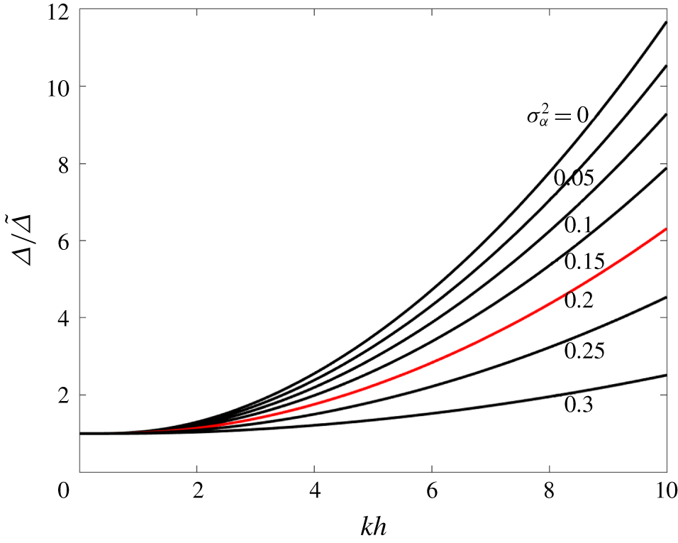
We note that the large  $k$ asymptote of
 $P\rightarrow (1/3-\unicode[STIX]{x1D70E}_{\unicode[STIX]{x1D6FC}}^{2})/(1-\unicode[STIX]{x1D70E}_{\unicode[STIX]{x1D6FC}}^{2})$, independent of
 $kh$, and thus the value of
 $\unicode[STIX]{x1D6E5}$ is not asymptotic to zero as
 $k\rightarrow \infty$. As a result, shear instability is not guaranteed in the large wavenumber limit. Finally, the two stability criteria (5.7) and (5.14) have the same overall form, and do not show any additional effects that would indicate the basic trough instability of Reference Madsen and FuhrmanMF20.
6 Discussion and conclusions
The model derived in § 3.2 provides guidance on the development of low-order FNBTE for practical application which should not be subject to the same type of noise observed in past applications based on finite difference calculations. The development of model equations for practical application requires inclusion of variable water depth and would generally be developed based on the Euler equations in order to incorporate vorticity in the horizontal flow field. This work will be reported separately.
The form of most FNBTE allows the volume flux to be specified as total depth multiplied by an expression representing depth-averaged horizontal velocity, allowing the flux to drop naturally to zero at the wet/dry boundary. This property, which is not satisfied by BTE written in terms of a velocity other than the depth-averaged velocity (e.g. Nwogu Reference Nwogu1993), greatly enhances model stability near shorelines. However, as pointed out by Bellotti & Brocchini (Reference Bellotti and Brocchini2002) (see also Durán, Dutykh & Mitsotakis (Reference Durán, Dutykh, Mitsotakis, Abcha, Pelinovsky and Mutabazi2018)), this feature of FNBTE is not sufficient to suppress apparent shoreline instabilities in models such as Wei et al. (Reference Wei, Kirby, Grilli and Subramanya1995), where dispersive terms do not approach zero at the shoreline boundary. The present model, or any model where dispersive terms are written entirely in terms of total depth  $H$, have this property and are not subject to the instability discussed by Bellotti & Brocchini (Reference Bellotti and Brocchini2002).
The model of § 3.2 complicates the interpretation of results in engineering calculations somewhat, as the velocity variable  $\boldsymbol{u}_{\unicode[STIX]{x1D6FC}}$ is the component of velocity of a particle in the tangent plane of a constant
 $\unicode[STIX]{x1D70E}$ surface, rather than a horizontal velocity in physical Cartesian coordinates, as in Wei et al. (Reference Wei, Kirby, Grilli and Subramanya1995) or KKCD01. Comparing the model of KKCD01 to the present model, the change in variables leads to a more complex conservation equation for volume but greatly simplifies the form of dispersive terms in the momentum equation. Physical velocities expressed at fixed
 $z$ elevations would be found by determining the
 $\unicode[STIX]{x1D70E}$ value at the desired
 $z$ and local values of
 $h(\boldsymbol{x})$ and
 $\unicode[STIX]{x1D702}(\boldsymbol{x},t)$, after which the horizontal velocity in physical coordinates is given by
 $\boldsymbol{u}=\boldsymbol{u}_{\unicode[STIX]{x1D6FC}}+\unicode[STIX]{x1D735}\tilde{\unicode[STIX]{x1D719}}_{2}\unicode[STIX]{x1D70E}(z)^{2}+2\unicode[STIX]{x1D70E}\tilde{\unicode[STIX]{x1D719}}_{2}\unicode[STIX]{x1D735}\unicode[STIX]{x1D70E}$. On the other hand, the model described here provides a natural setting for determining quantities at the free surface, as in, for example, the determination of wave breaking criteria based on values of the horizontal particle velocity at the free surface (Barthelemy et al. Reference Barthelemy, Banner, Peirson, Fedele, Allis and Dias2018; Derakhti et al. Reference Derakhti, Kirby, Banner, Grilli and Thomson2020). We conclude that trough instability is not an intrinsic feature of FNBTE and can be eliminated by derivations that produce equations with total layer depth as the only measure of layer thickness in dispersive term coefficients.
Acknowledgements
This work was supported by the National Science Foundation, Physical Oceanography Program grant OCE-1948705 to the University of Delaware. P. Guyenne and the referees are thanked for providing references for the internal wave problem and various aspects of the free-surface problem.
Declaration of interests
The authors report no conflict of interest.