2.1 Description logics

DLs (Baader & Nutt, Reference Baader, Nutt, Baader, McGuinness, Nardi and Patel-Schneider2010) is the name given for a family of knowledge base representation (KR) formalisms used to represent domain knowledge by defining a terminology (the relevant concepts in the domain), then using these concepts to describe properties of individuals in the domain. The terminology and the information about the individuals form the knowledge base.

DLs are particularly useful for the Semantic Web because most of them are decidable fragments of the FOL. Hence, when the DL is decidable, a query is always answered, either positively or negatively. However, the decidability and complexity depend on the DL language chosen. Usually, there is a trade-off between expressiveness and the reasoning complexity, as a higher expressive power may incur in a higher reasoning complexity.

In a DL language, there are three types of entities: atomic concepts, atomic roles and individual names. Atomic concepts and roles are the elementary descriptions in a DL language. Complex descriptions, or descriptions in short form, can be built from atomic concepts and roles using concept constructors. DLs languages are distinguished by the set of constructors they provide; therefore, the expressiveness of a DL is tied to its set of constructors. In the remainder of this work, we use the letters $a, b, a_1, b_1,\ldots$ for individuals; the letters $A, B, A_1, B_1, \ldots$ for atomic concepts, the letters $R, R_1, \ldots$ for atomic roles and the letters $C, D, C_1, D_1, \ldots$ for concept descriptions. A definition has the form $A \equiv C$ or $A \sqsubseteq C$ , although here we focus only on the first type. One can see that a definition has an atomic concept on its left side and a concept description on the right side. A concept assertion has the form A(a) and a role assertion has the form R(a, b).

In this manuscript, we adopted the $\mathcal{ALC}$ (Attributive Concept Language with Complements) language (Baader & Nutt, Reference Baader, Nutt, Baader, McGuinness, Nardi and Patel-Schneider2010) motivated by the fact that it constitutes the foundation of other DLs. In this case, the syntax of the definitions belonging to the set of $\mathcal{ALC}$ concepts are as follows: (i) $\lnot C$ is the negation of a concept; (ii) $C \sqcap D$ is the intersection of two concepts; (iii) $C \sqcup D$ is the union of two concepts; (iv) $\forall\,R.C$ is the universal restriction of a concept by a role; and (v) $\exists R.C$ is the existential restriction of a concept by a role.

The most frequently used way of defining $\mathcal{ALC}$ semantics relies on the definitions of interpretation, model and fixpoints over a domain (Baader & Nutt, Reference Baader, Nutt, Baader, McGuinness, Nardi and Patel-Schneider2010). Thus, here, the semantics of a description is given by a domain $\mathcal{DOM}$ (a set) and an interpretation $\cdot^{\mathcal{I}}$ (a functor). Individuals represent objects through names from a set $N_\mathsf{I} =\{a,b,\ldots\}$ . Each concept in the set $N_\mathsf{C}=\{C,D,\ldots\}$ is interpreted as a subset of a domain $\mathcal{DOM}$ . Each role in the set $N_\mathsf{R} = \{r,s,\ldots\}$ is interpreted as a binary relation on the domain.

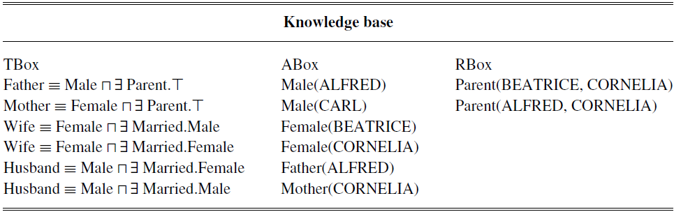
An ontology in DL consists of a set of statements called as axioms (Krötzsch et al., Reference Krötzsch, Simancik and Horrocks2012). In DL, an ontology represents the knowledge base; therefore from now on, we use the expressions knowledge base and ontology interchangeably. Thus, a knowledge base in DL has three components: the TBox, the ABox, and the RBox. TBox axioms describe relationships (e.g. inclusion and equivalence) among concepts in the form of terminological knowledge, that is, the domain’s vocabulary. ABox axioms accommodate assertions about named individuals using the terms defined in the terminology, aiming at expressing a relationship between a concept and an individual. RBox axioms assert relationships between named individuals. The Table 1 shows an example of a knowledge base with these three components.

Table 1

Example of a knowledge base comprising three components, a TBox (terminological axioms) and a ABox (assertional axioms), and RBox (relational axioms)

In this paper, we assume the common assumptions made about DL terminologies: (i) there is only one definition for a concept name and (ii) the terminology is acyclic. Here, we say that a terminology is acyclic if there is no cycle in the taxonomy tree built from the concepts. Attached to a DL, there must be a reasoning mechanism, responsible for inferring knowledge about individuals using the knowledge base.

In this paper, we define the length of a description according do Definition 1.

For example, considering the last concept definition exhibited in Table 1, Husband $\equiv$ Male $\sqcap\,\exists$ Married.Male, the length(Husband) = 5, which is the number of terms after the $\equiv$ symbol in the description Husband.

2.2 Concept learning

In order to effectively exploit terminologies over a domain, especially when dealing with large amounts of data such as in the Semantic Web (Berners-Lee et al., Reference Berners-Lee, Hendler and Lassila2001), it is useful to apply techniques from machine learning (Mitchell, Reference Mitchell1997) for automatically inducing terminologies from data.

Since concepts are the basic component of a terminology, the first step is to conceive how to automatically learn a concept from available data. A number of algorithms together with implementations have been proposed in the literature to learn concepts in DL (Iannone et al., Reference Iannone, Palmisano and Fanizzi2007; Fanizzi et al., Reference Fanizzi, d’Amato and Esposito2008; Lehmann, Reference Lehmann2009; Lehmann & Hitzler, Reference Lehmann and Hitzler2010; Lima et al., Reference Lima, Espinasse and Freitas2018; Ozaki, Reference Ozaki2020). They are inspired on techniques developed within the field of Inductive Learning Programming (ILP) (De Raedt, Reference De Raedt2008), whose general goal is to automatically induce logic programmes from data. When learning a concept, one has as goal to find a generalised and correct definition of such a concept from a set of examples, as defined below:

Although Definition 2 requires that the learned concept covers all the positive examples and none of the negative examples, usually this hard criteria is relaxed, to achieve a definition as good as possible.

Logic-based systems that learn concepts often compare candidates through scoring functions based on the number of positive/negative examples covered. In DL-Learner, for example, a fitness relationship considers the number of positive examples and negative examples covered as well as the length of solutions when expanding candidates in the tree search.

3.1 Finding concept dependencies through examples (CDE)

The CDE method finds a suitable learning order, according to a dependency taxonomy built from the examples. In this way, a concept learned at iteration i can be included in the definition of concepts learned after iteration i. This method relies on the assumption that by finding out the subsumption relationship between concepts, it is possible to yield an ordering of the concepts, which in return will support the learning of a rich — although simple and easily readable — terminology.

The question that arises is how to obtain a subsumption order from concepts that do not have definitions yet, that is, before their definitions are learned. We tackle this problem by developing a procedure capable of finding out the relations among concepts before learning them, by taking advantage of their set of examples. Because of the completeness and consistency properties of the concept learning task, the set of positive and negative examples provides strong evidence for the existence of dependencies and relationships among concepts.

Let ${LT_A}_i=<\mathcal{KB},\mathcal{E}_{A_i}^{+} \cup \mathcal{E}_{A_i}^{-}>$ and ${LT_A}_j=<\mathcal{KB},\mathcal{E}_{A_j}^{+} \cup \mathcal{E}_{A_j}^{-}>$ concept learning tasks for concepts $A_i$ and $A_j$ , respectively. After learning descriptions for these concepts, their definitions will be part of the TBox. Therefore, a comparative analysis of the individuals belonging to $\mathcal{E}_{A_i}^{+}$ and $\mathcal{E}_{A_j}^{+}$ could point out how strongly related the corresponding concepts are and what might be the best order ( $\preccurlyeq$ ) for learning them. Briefly, we argue that high similarity on the positive examples sets indicates high similarity between concept definitions. Example 1 illustrate this point.

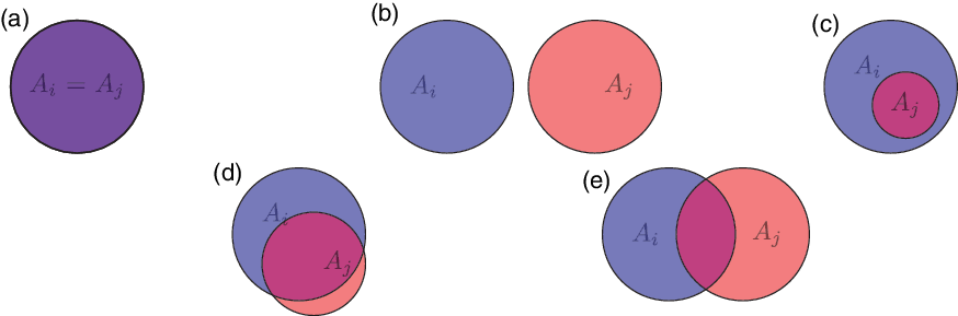
The comparative analysis between two concepts ( $A_i$ and $A_j$ ) through their sets of positive examples comprises the following five cases, illustrated at Figure 1:

1. (a) Identical sets ( $A_i \equiv A_j$ ): all elements belonging to one set also belong to the other set;

2. (b) Disjoint sets ( $A_i \cap A_j = \emptyset$ ): both sets have no elements in common;

3. (c) Inner set ( $A_i \subseteq A_j$ ): one set is a subset of the other;

4. (d) High intersection: the proportion of shared elements overcomes a threshold;

5. (e) Low intersection: the proportion of shared elements does not overcome a threshold.

Figure 1

The relationship among concepts $A_i$ and $A_j$ through their positive examples sets, represented as Venn diagrams

We claim that the higher is the intersection between sets of positive examples, the greater is the relationship between the concepts. Thus, case (a) describes an upper limit, where the concepts are totally related, while case (b) indicates a lower limit, where the two concepts have no relationship. Furthermore, cases (a), (b) and (c) are the ideal cases because the underlying relationships between concepts are clear; on the other hand, the cases (d) and (e) need some mapping to one of the ideal cases, as ‘high’ and ‘low’ depends upon the observer. This is accomplished via a threshold value that will indicate how the concepts are related to each other. Therefore, the case (c) is a special case of (d), when the threshold is equal to 1; the case (b) is a special case of (e), when the threshold is equal to 0.

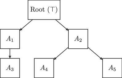
In this way, the relations among all concept definitions may be obtained from the comparative analysis of each pair of concepts that belong to the terminology learning task. The resulting explicit relations among the concepts are translated to a subsumption tree (a taxonomy). For instance, consider the taxonomy depicted in Figure 2 for the set of concepts $N_C = \{A_1,A_2,A_3,A_4,A_5\}$ .

Figure 2

An example of a taxonomy depicting the relation among concepts $A_1, A_2, A_3, A_4$ and $A_5$

The root node indicates the set of all individuals of the domain ( $\top$ concept). A concept in a branch on level i is more general than a concept on the same branch in level j ( $i<j$ ), thus concept $A_1$ is more general than concept $A_3$ . Assuming that a more general concept can be used in the definition of a more specialised one, the former should be learned first. Thus, the resulting taxonomy of the concepts can be used to determine the best ordering to learn the concept definitions.

3.1.1 Discovering a concept ordering

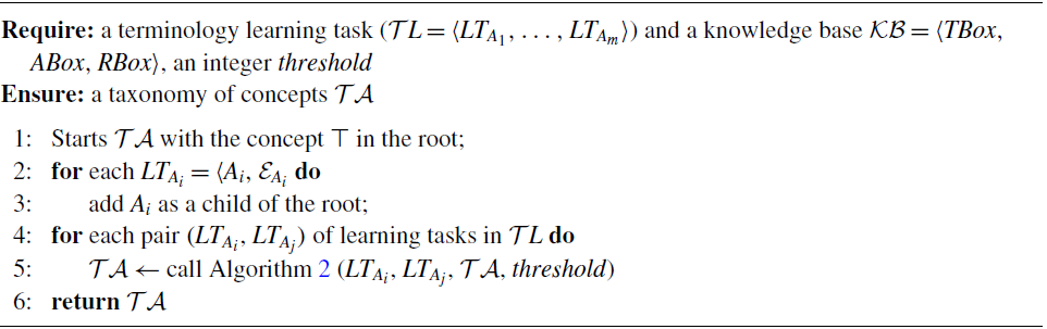
Algorithm 1 presents the top-level procedure for building a taxonomy of concepts that is used to define an order for learning the concepts of a terminology. It is based on the five possible cases previously discussed.

Algorithm 1

Algorithm for learning a taxonomy of concepts

The algorithm receives as input a terminology learning task, as outlined in Definition 3, and returns a taxonomy of its concepts. Given the ordering tree, a concept can only be defined if all its parents have already been defined. The root of the tree is a default concept which must be the parent of all the concepts in $\mathcal{T}L$ . This algorithm starts by creating a tree with only the root. Next, each concept ( $A_i$ ) corresponding learning task ( ${LT_A}_i$ ), where ${LT_A}_i \in \mathcal{T}L$ , is included in the tree as child of the root. Then, Algorithm 2 is called for each pair of concepts $A_i$ and $A_j$ in order to find their relationship. After checking each possible dependency, the final taxonomy of concepts is returned.

Algorithm 2

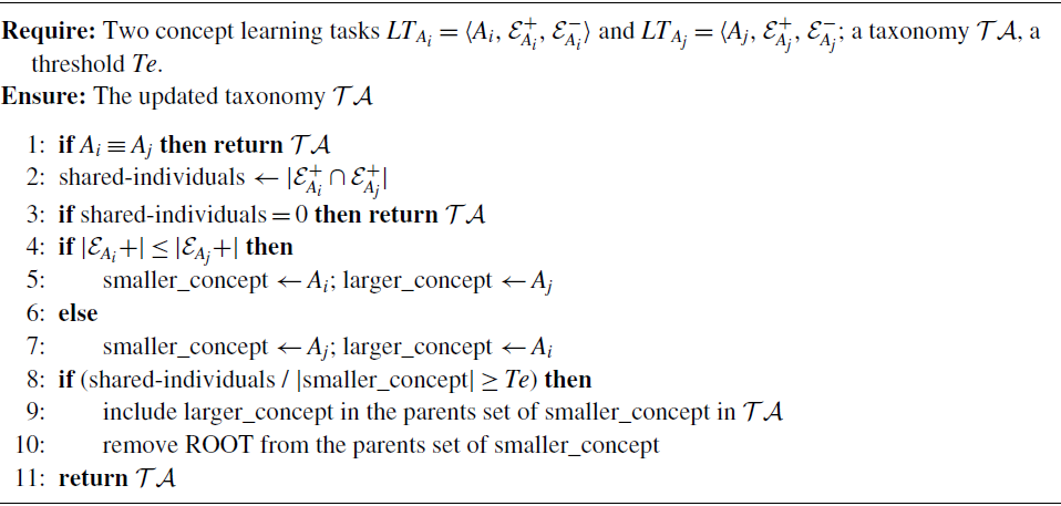
Algorithm for ascertaining dependencies among concepts in a terminology

In Algorithm 2, the relationship between the positive examples sets of the two concepts are analysed in order to resolve in which of the five cases discussed above it belongs. In case a pair of concepts are evaluated as equivalent, both of them are kept in the tree, making possible to learn a proper concept to each of them. It may be the case that during the learning, the negative examples point out that they have some difference. This also happens when the set of examples of two concepts is disjoint (Völker et al., Reference Völker, Fleischhacker and Stuckenschmidt2015).

When a set of examples is a subset of another one, we assume that the concept with the super set is more general than the other, called here as a subsumer. The concept with the subset is called subsumee and put as a child of the subsumer in the tree. Thus, the edge connecting the subsumee concept and the root is removed.

Finally, by employing a threshold parameter, we decide the type of relationship of two concepts that have intersected sets. If the proportion of shared individuals is higher than a threshold, we assume that the concept with more examples is a subsumer while the other is a subsumee.

3.1.2 Learning terminologies through concept ordering

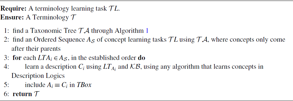
Algorithm 3 presents the overall procedure for learning a terminology using the CDE method. It requires as input the terminology learning task $\mathcal{T}L$ . The first step of the algorithm is to call the procedure devised as Algorithm 1, which is going to return the taxonomy tree comprising each concept addressed by the terminology problem.

Algorithm 3

Top-level algorithm for learning terminologies

Next, to find the order that the concepts are going to be learned, the nodes are collected in a breadth-first manner. For instance, considering the taxonomy in Figure 2, the concepts would be learned in the order $<A_1,A_2,A_3,A_4,A_5>$ . In this way, it is possible to guarantee that a concept is only handled after the descriptions of all its parents have been learned either.

Finally, to learn a description, the concept itself, its positive and negative examples and the current background knowledge are submitted to a DL learning algorithm, such as DL-Learner (Lehmann & Hitzler, Reference Lehmann and Hitzler2010), DL-FOIL (Fanizzi et al., Reference Fanizzi, d’Amato and Esposito2008) or Yin-Yang (Iannone et al., Reference Iannone, Palmisano and Fanizzi2007). Then, the description found is included in the TBox of each $\mathcal{KB}$ of the following ${LT_A}_i$ , so that it can be used in next iterations of the loop, as part of other descriptions.

3.2 Finding dependencies during the learning phase (CDA)

The CDE approach defines an arguably ideal dependency order for the concepts and strictly follows such an order when learning the descriptions. This is required by the learning phase as it is not possible to use an ‘unknown’ non-atomic concept, that is, a non-atomic concept without a description, when inducing a description for another concept. However, defining such an order before the learning phase has the disadvantage of not taking into account what is actually being learned to find possible dependencies between concepts. Thus, one question that arises is how the definition for a concept $A_j$ can be considered in the description of another concept $A_i$ before the description for $A_j$ has been actually learned? The way we answer this question is devising the procedure CDA, that makes the concepts look like atomic ones. For achieving that, the examples of a concept are transformed into assertions in the ABox, defining a new ABox: $ABox' = ABox \cup {\mathcal{E}_{A_i}^{+}} \cup \neg {\mathcal{E}_{A_i}^{-}}$ , where $\neg {\mathcal{E}_{A_i}^{-}}$ is the set of negative assertions for the concept $A_i$ ; it specifies the individuals that are not elements of $A_i$ .

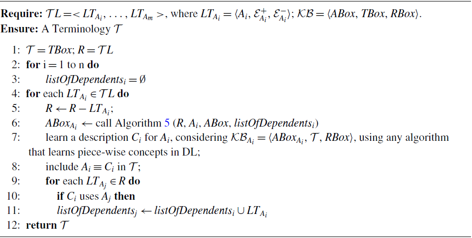
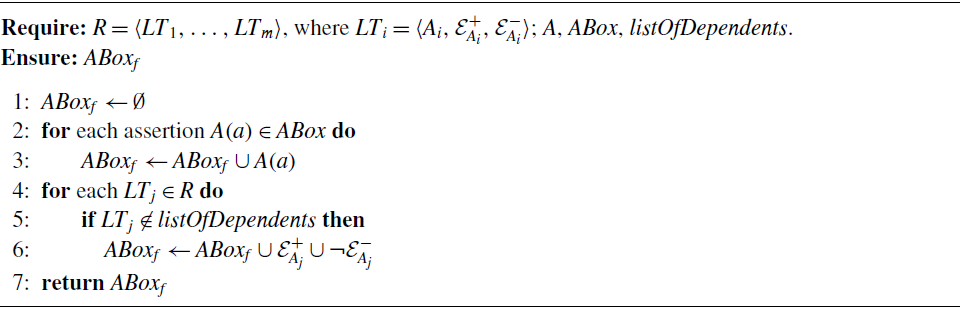
CDA top-level procedure (Algorithm 4) works like that: for a particular learning task ${LT_A}_i \in \mathcal{T}L$ , all other concepts $A_j$ , where ${LT_A}_j \in \mathcal{T}L\setminus {LT_A}_i$ and $A_j$ was not already learned, are transformed into atomic concepts available to be used during the learning phase for $A_i$ (Algorithm 5). For the successful use of this approach, there are some conditions that must be observed, as stated in Restriction 1.

Restriction 1 (CDA’s Restrictions) The following are restrictions for the proper work of the method CDA:

1. 1. All the concept learning tasks must share the same ABox, that is, they all should encompass the same set of individuals.

2. 2. All the relevant individuals for a particular concept learning task should appear in one of its example sets (completeness).

3. 3. The background knowledge is a finite model.

4. 4. For every concept A in terminology learning task $\mathcal{T}L$ and every individual I relevant to the concept A, $I \in {\mathcal{E}_{A}^{+}}$ or $I \in {\mathcal{E}_{A}^{-}}$ .

Algorithm 4

CDA (avoiding cycles)

Algorithm 5

Algorithm to find virtual atomic concepts

Those are reasonable constraints as the amount of information on $\mathcal{E}$ tends to yield better resultsFootnote ² .

When CDA’s restrictions are uphold, it is possible to use the sets of examples $\mathcal{E}_{A_i}$ of each concept learning task within a terminology learning task $\mathcal{T}L = <{LT_A}_1, \ldots, {LT_A}_m>$ , as a surrogate for the definition that will be found later, with no semantic lost. There is no difference with regard to the result obtained from the reasoning services for a query A(a), whether it is an assertion (ABox) or if it follows an inference process using the terminology (TBox). An additional benefit is that each concept learning task can be executed independently, allowing for parallel learning of each concept.

Moreover, CDA procedure can overcome CDE bias for concept/subconcept ordering which may yield more concise terminologies. CDE is tuned to find relations of the type subsumer and subsumee, for example, in the kinship domain we have $\mathsf{GRANDFATHER} \sqsubseteq \mathsf{FATHER}$ . However, it cannot reliably work with different relations, for example, the union of $\mathsf{GRANDFATHER}$ and $\mathsf{GRANDMOTHER}$ to define $\mathsf{GRANDPARENT}$ . CDA is capable of dealing with it because we turn the learning task into the responsible component for finding relationships between concepts.

Example 2 shows the output of the terminology learning task for the set of concepts {GRANDPARENT(GP), GRANDMOTHER(GM), GRANDFATHER(GF)}.

Unfortunately, as the example shows, the terminology learned in this fashion may introduce a new problem, as cycles may be formedFootnote ³ . This goes against one of the general assumption we need to uphold—concept definitions are acyclic. We propose two approaches to deal with cycles: (i) restrict the set of examples added to $\mathcal{KB}$ and (ii) remove the cycles on a post-procedure.

1. (i) If a concept $A_j \in \mathcal{T}L\setminus LT_{A_i}$ , $i\not = j$ , already has a definition and it uses $A_i$ do not include $A_i$ or $A_j$ in $\mathcal{KB}$ . This prevents that any new definition creates a cycle. As a consequence, an order for the learning process may be necessary. In this case, the best acyclic solution is not guaranteed.

2. (ii) After the end of the learning phase, to identify the concepts that incurred in cycles and relearn them, avoiding the current or a recurring cycle. Choose the definitions that yield smaller definitions.

The second method has a better chance to return the optimal acyclic solution, but it may relearn several concepts. In both methods, the best acyclic solutions is not guaranteed.

3.2.1 CDA with cycle removal

The first proposed method only deals with cycles with depthFootnote ⁴ of one, as exemplified in Example 3.

Example 3. The terminology containing the concepts: $A \equiv B_1 \sqcap B_2 \sqcap B_3$ and $B_1 \equiv B_4 \sqcap B_3 \sqcup A$ has a cycle with depth of one, because the concept A appears in the definition of $B_1$ while it also uses $B_1$ within its own description description, needing only one inferential step before incurring in a cycle.

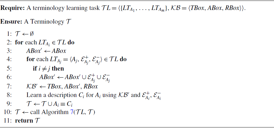
Algorithm 6 is the entry point for the learning process. It runs the CDA for the terminology learning task and call the Algorithm 7 to remove the cycles of the learned terminology.

Algorithm 6

CDA with cycle removal main algorithm

Algorithm 7

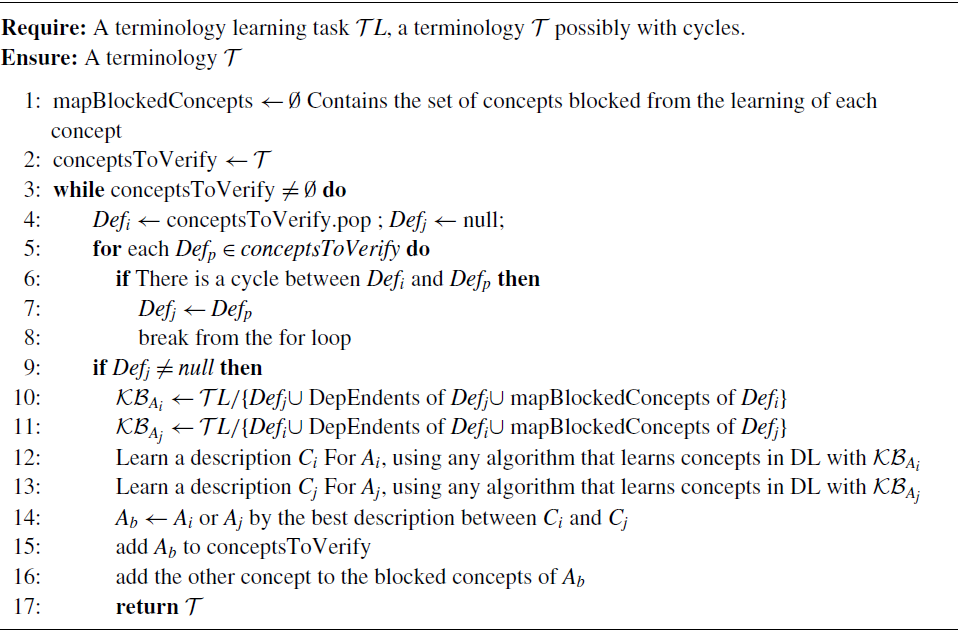
Algorithm for removing cycles from the learning tasks

Algorithm 7 is used to remove the cycles of a set of concept learning tasks. It starts by defining an empty map of blocked concepts. A concept $A_j$ is a blocked concept for the learning of a concept $A_i$ , if in a previous iteration there was a cycle between $A_i$ and $A_j$ and $A_i$ ’s definition was altered. Furthermore, it creates a set of concepts that are in need of cycle verification, beginning with all the concept learning tasks.

While there are concepts to check for cycles, it chooses two concepts within this set to verify if there is a cycle involving them. If a cycle exists between two concepts, it creates a new $\mathcal{KB}$ using the existing $\mathcal{KB}$ together with the set of concepts not blocked (lines 10, 11). All the dependents of a blocked concept are themselves blocked concepts. Finally, alternative definitions are learned for both concepts using their ‘new’ $\mathcal{KB}$ s.

Once the alternative definitions are acquired, one must choose which of the two concepts will receive the alternative definition (line 14). The choice is made in favour of the alternative definition with the smallest impact on the terminology, that is, the one with least difference in length with regard to the original definition. Lastly, the concept learning task whose definition was altered has to be verified, because new cycles may have been introduced, and the other concept learning task is added to alter concept’s blocked set.

3.3 Finding dependencies on an existing terminology (CDT)

Finally, we devise a method that is able to find dependencies among concepts even in a ready-to-use terminology. It aims at compactness, since it finds parts of a concept description that can be replaced by a single concept. It is motivated by the fact that if part of the description has a semantically equivalent but syntactically smaller counterpart, then a substitution could take place generating a smaller though equivalent definition. Henceforth, we call this process syntactic compression.

3.3.1 Syntactic compression using a tree representation

In order to achieve a syntactic compression, it is necessary to find viable substitutions, that is, parts of a concept definition that encompass another concept.

At a first glance, the syntactical compression may be done performing a simple matching of the two logical definitions. However, this approach is very likely to not produce all possible substitutions, since most of the DL’s constructors are commutable, as shown in Example 4.

Example 4. The logical definition $A \sqcap B_1 \sqcap B_2$ is equivalent with any conjunction of permutations of the concepts $\{A, B_1, B_2\}$ , such as: (i) $A\sqcap B_2 \sqcap B_1$ , (ii) $B_2 \sqcap A \sqcap B_1$ , …

In order to overcome this limitation, while still performing a syntactic compression, we propose the use of a n-tree representation of the concepts definitions, whose (i) internal nodes represent a constructor, (ii) leaves represent concepts and (iii) all the children of a constructor node are commutable. Allowing the commutation of the constructor’s node children is essential, since identical definitions, unless for the order of literals, should have the same associated tree. This is illustrated in Example 5.

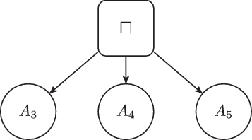
Example 5. Let $A_1,A_2,A_3,A_4,A_5$ concepts in a terminology, such that concept $\mathsf{A_1}\equiv A_3 \sqcap A_4 \sqcap A_5 $ and $\mathsf{A_2} \equiv A_5 \sqcap A_3 \sqcap A_4$ . Figure 3 shows the representation for both concepts:

Figure 3

Example 5’s syntactic tree representation

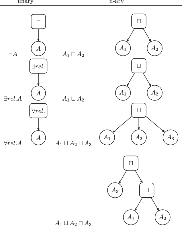
Figure 4 shows all the correlations between $\mathcal{ALC}$ ’s constructors and their tree representation. We stress that the proposed method is language-independent as long as it is possible to separate the constructors of the DL language between unary and binary (commutable n-ary) constructors.

Figure 4

The syntactical tree representation of $\mathcal{ALC}$ ’s constructors

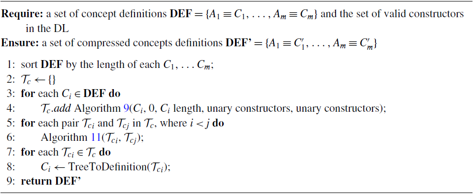
Removal of redundant descriptions. Algorithm 8 presents our procedure to syntactically compress a terminology. It receives as input a terminology and the set of available constructors, divided into unary and n-ary, and returns (possibly) compressed terminology. It starts by sorting the set of concepts in an ascending order of length, as a concept can only have a substitution involving a smaller concept. Next, for each concept in the terminology, it finds its corresponding tree form (line 4).

Algorithm 8

Syntactical compression main algorithm

Once it has the tree representation with all concepts, it can proceed to find suitable substitutions. It does so by exhausting all the pairs of concepts with a smaller concept and a larger one (line 5), and calling Algorithm 11 (line 6) to find a proper substitution. After all the substitutions are made, it changes the modified original concept definitions by translating the tree representation back to its logical form (line 8). The translation method is done via a pre-order traversal in the tree.

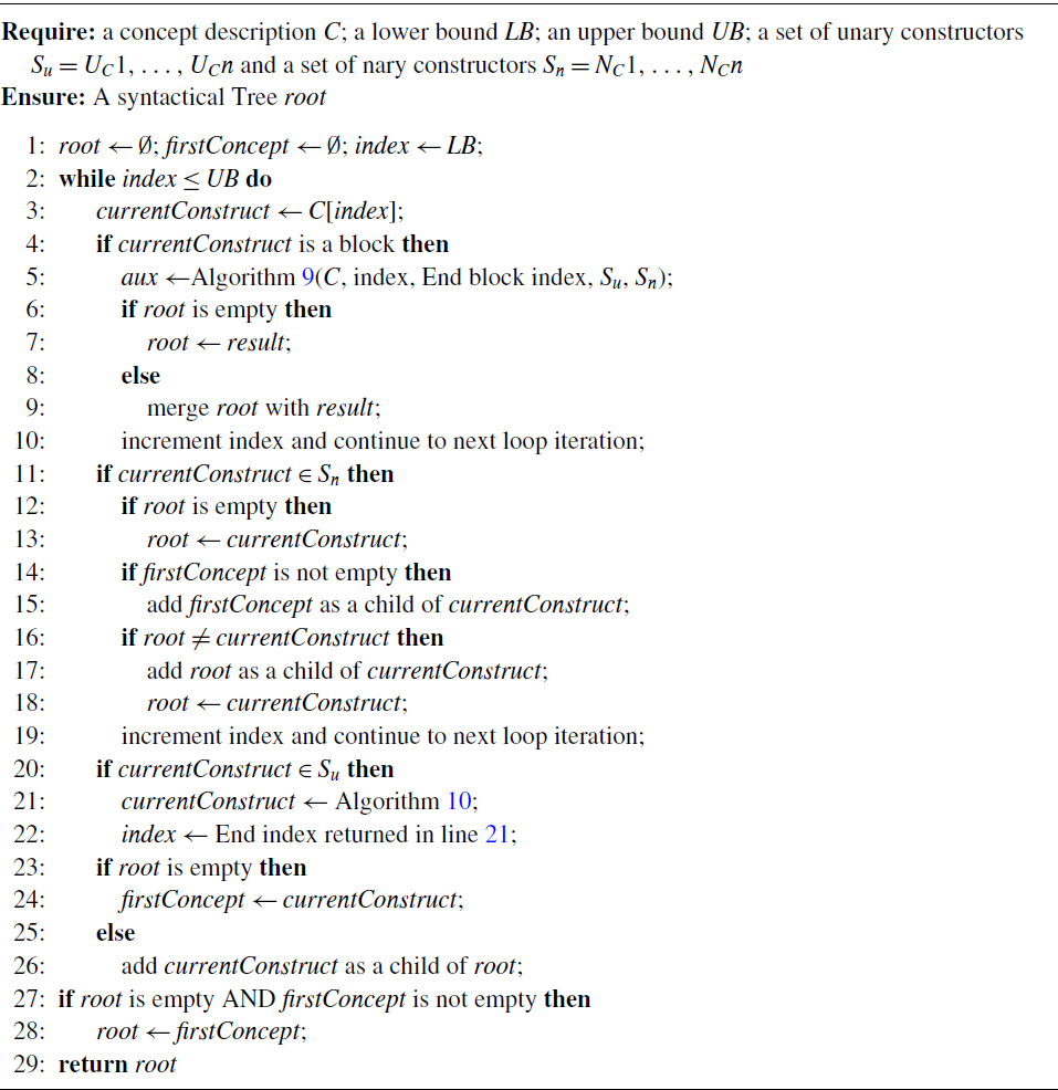
Syntactic tree construction. Algorithms 9 and 10 are used to parse the logical syntax into the tree representation. In case all the n-ary constructors have the same precedence, as it is the case of $\mathcal{ALC}$ language, we still need a way to distinguish them in the tree. We do so by creating a hierarchy in the tree with them. Thus, the line 16 of algorithm 9 creates a subtree as soon as it identifies a constructor different from the previous one. In case the DL language defines a different precedence rule than $\mathcal{ALC}$ , the algorithm must be changed to attend such a rule.

Algorithm 9

Converting a logical description to a syntactical tree

Algorithm 10

Recursive method for unary constructors

In the syntactic representation, a block is a part of the definition enclosed within parenthesis, and it may contain other blocks. The upper and lower bound are the begin and end of a concept or block, respectively.

Finding proper substitutions. Algorithm 11 is used to perform substitutions between two trees, a larger tree and a smaller tree. To perform a substitution, it must find a node within the larger tree that is the root of the smaller tree (line 4). In this representation, a larger tree contains a subtree equivalent to a smaller tree when: (i) all the internal nodes in the smaller tree have an equivalent node in the larger tree (also with equivalent arcs), and (ii) the subtree root of the larger tree contains all the nodes below the smaller tree root. Example 6 shows why the second constraint does not state that the larger tree subtree’s root should be equal to the smaller tree’s root. The problem of finding an equivalent tree is also known in the literature as tree isomorphism (Zemlyachenko et al., Reference Zemlyachenko, Korneenko and Tyshkevich1985).

Algorithm 11

Syntactical compression’s substitution

Example 6. Let $A_6\equiv A_1 \sqcup A_2 \sqcap A_3$ and $A_5 \equiv A_1 \sqcup A_2$ . Executing the substitution on the tree representation of $A_6$ and $A_5$ we have

4.1 Datasets

The domains considered in this work are as follows:

• The Kinship domain defines family relations through a terminology containing three roles, sibling, married and parent, and two atomic concepts, male and female. The concepts that should be learned are Grand Parent (GP), Grand Father (GF), Grand Mother (GM), according to their standard semantic.

• Moral reasoner (Wogulis, Reference Wogulis1994): this dataset describes moral statements such as ‘Someone is guilty of an action if it is blameworthy or he/she takes the blame for someone else’. It has a terminology composed of 25 atomic concepts and 20 non-primitive concepts. The ABox has assertions for 202 individuals. However, not all the assertions about non-primitive concepts are represented, in these cases it is necessary to infer them. Two experiments were done with this dataset. In the first one (Exp1), the concepts that must be learned are {guilty, blameworthy, responsible, notaccident}, and in the second one, (Exp2), {guilty, blameworthy, responsible, notaccident, weak_intend, intend_c}, increasing the learning process complexity with two more concepts. The concepts for each set of problems were chosen because of their inter-dependencies.

• OAEI campaign: different from CDA and CDE, CDT method can deal with terminologies that do not have individuals (ABox) because it works only with concept’s descriptions (TBox). Because of that, we experiment CDT using a number of datasets from OAEIFootnote ⁵ campaign of ontology matching and all datasets packaged as examples on DL-Learner systemFootnote ⁶ . In total, there were 46 datasets with a wide range of domains, for example, the kinship, moral, biomedical, and sizes, ranging from 0 to 10 480 complex concepts.

4.2 Individually experimenting each method

In this section, we experimentally evaluated each of the three approaches.

4.2.1 CDE: Finding the best threshold value

CDE uses a threshold parameter to define a lower limit for the proportion of intersection of the examples associated with two concepts, after which the concepts are considered dependent by the method. In Melo et al. (Reference Melo, Revoredo and Paes2013a), the threshold value was arbitrarily set to 80%. Here, we empirically experiment on several values to decide which one is the best for the threshold parameter.

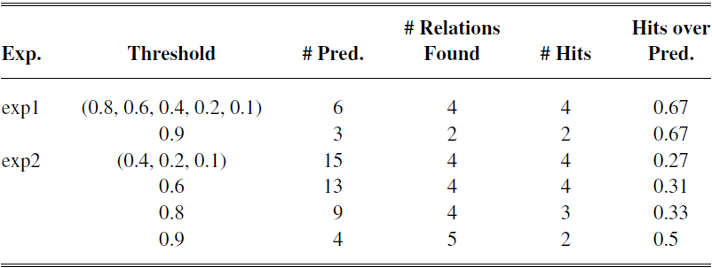
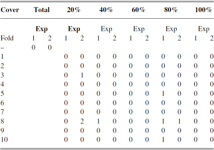
Thus, to analyse the behaviour of CDE approach according to the threshold parameter, we set it to 20%, 40%, 60%, 80% and 90% and compute the matching relationships using the moral reasoner dataset. Table 2 presents the average predictive results. The second column presents the threshold’s value, aggregating them in the cases where the corresponding results are the same. The third column shows the number of predictions returned by the induced taxonomy and the fourth column shows the subset size of relationships that were indeed considered in the learned terminology. The fifth column shows the number of found dependencies that matched those presented in the target description, we called this metric as Hits. The results indicate that indeed the $80\% $ threshold is a good value, followed closely by 90%. As it should be expected, requiring only a low intersection between two sets of examples yields a high number of predictions that are not actually established during the learning phase.

Table 2

CDE: Best threshold experiment. Hits indicate the number of found dependencies that matched those presented in the ground truth

4.2.2 Experimenting CDA

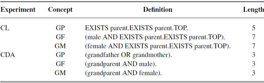
CDA adds the learning examples to the background knowledge in order to induce the shortest solution, in terms of the length of the description, for a single concept learning task. We devised an experiment using the Kinship domain in order to validate this claim. In this experiment, we do not uphold the assumption that the terminology must be acyclic, since we would like to know if CDA’s surrogates are indeed correct and can yield the shortest description for all the concepts in a terminology learning task. Table 3 shows the result for this experiment contrasting with the result achieved with the concept learning (CL) method.

Table 3

CDA’s validation experiment results

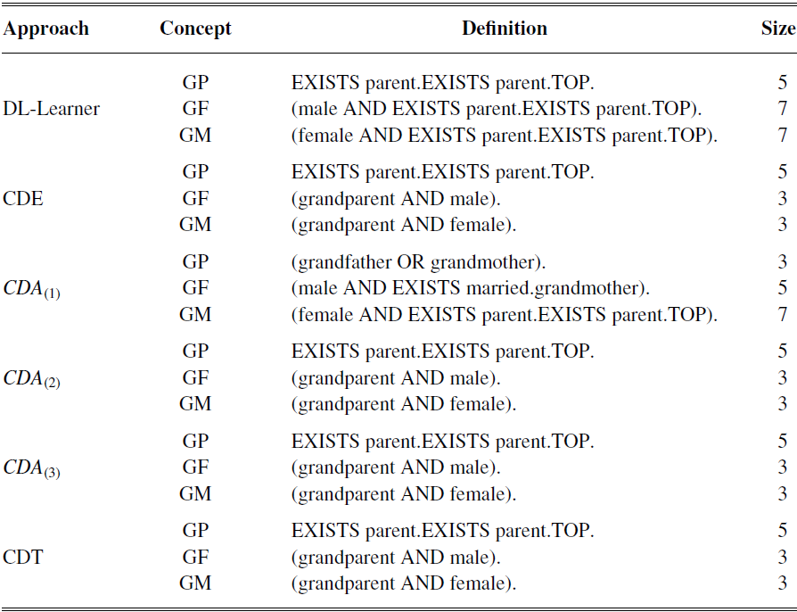
CDA achieves a terminology of length nine, while the single concept learning system DL_Learner found a terminology of length nineteen. Furthermore, CDA founds the shortest possible solution for all the three concepts in the terminology learning task.

4.2.3 Experimenting CDT

Different from the CDE and CDA methods, CDT can be used outside the terminology learning problem, because it is a method for theory restructuring. Table 4 presents the results obtained with CDT, but only to the cases that it was able to get some difference in the terminology.

Table 4

CDT: Results of the validation experiment, showing only the datasets that a different terminology was yielded

The method achieved syntactic compression on only 3 of the 46 terminologies: conf_Cocus, NCI_small_overlapping_fma.owl and NCI_whole_ontology.owl. In the conf_Cocus domain, the original terminology is composed of five complex concepts (Administrator, Document, Event, Event_Setup and User), ‘with Document’ and ‘Event’ having the same definition: ‘ $\exists created\_by.Person$ ’. The method arbitrarily substituted one of the definitions by the other concept, for example, returning the description $Event \equiv Document$ . In this particular case, it might be argued that the real meaning is lost when this substitution is performed, but from a pure logical point of view the semantic is maintained.

The other remaining Biomedicine domains share much of the concepts and descriptions. In fact, the terminology of NCI_whole_ontology.owl contains the NCI_small_overlapping_fma.owl. Both had the same two substitutions: the concept ‘Complement_Component-4’ was substituted by its definition on concepts ‘Complement_Component-3’ and ‘Complement_Component-5’. Both concepts where the substitution occurred have a structure of many conjunctions of existential restrictions. These particular replacements are difficult to visualise because of the size of the descriptions (41 and 57, respectively). This might suggest a direct relationship between a terminology size and its complexity and how difficult it is to find all the simplifications manually.

Regarding the cases where CDT made no difference, we observed two situations: (1) a number of these datasets have only atomic concepts and roles in the ABOX but no concepts definitions to compress and (2) in the other cases, the method had no impact on the size of the terminology, as they were already syntactically compressed. More than anything, this might be a testament of the quality of the terminologies.

4.3 Experiments comparing the three methods

In this section, we describe experiments conducted towards comparing CDE, CDA and CDT, among each other and to a standard single concept learning system, namely DL-Learner. It is necessary to define the knowledge base ( $\mathcal{KB}$ ) and the sets of examples ( ${\mathcal{E}_p}_i$ , ${\mathcal{E}_n}_i$ ) for each concept learning ${A_C}_i$ . The latter is performed either directly from the original examples or by performing inference along the terminology and the knowledge base. While the $\mathcal{KB}$ is the same in all ${A_C}_i$ , ${\mathcal{E}_p}_i$ and ${\mathcal{E}_n}_i$ vary in accordance with the concept. The experiments are conducted on the Kinship and moral reasoner datasets, previously described.

4.3.2 Experimental results

Kinship dataset. The results obtained considering the Kinship dataset are depicted in Table 5.

Table 5

Toy example results: Concepts definitions and their sizes found with the methods CDE, CDA, CDT and DL-Learner (DL-L)

From that, it is possible to see that all the concepts description follow the correspondent semantics. Moreover, CDE, CDA and CDT were able to learn a more concise and readable terminology than DL-Learner. Additionally, in order to uphold DL’s assumption of acyclic terminologies we used: a version of CDA that avoids cycles ((1) and (2)), in this case orderings are particularly important, that is, different orders entail different results; and a version of CDA that removes the cycles (3) (Algorithms 6 and 7). The results in Table 5 supports such conclusion and shows that CDA avoiding cycles is able to achieve the same terminology as CDE and CDT by reversing its learning order.

Moral reasoner dataset. In the rest of this section, we will refer to CDA avoiding cycles as $CDA_1$ or CDA1, and to CDA removing cycles as $CDA_2$ or CDA2.

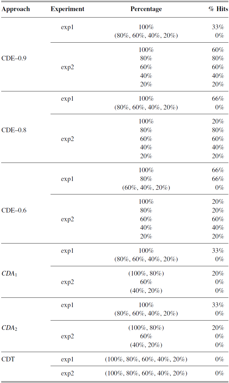
Table 6 exhibits the results for all the proposed approaches (CDE, CDA1, CDA2 and CDT), considering the two experiments (Exp1 and Exp2) described in Section 4.3.1 and different percentages of the training examples. The proportion of positive and negative examples was maintained in each set. Regarding CDE, we present the results for three different values of the threshold parameter (60%, 80%, 90%). Moreover, to evaluate the approaches, we considered the percentage of original dependency among concepts found in the learned terminology (% Hits) and Table 6 depicts the average of the 10 folds.

Table 6

Aggregate results of relaxing completeness experiment for the methods CDE, CDA and CDT

Observing the results in Table 6, both CDE and CDA performed worse than expected. The CDA (1 and 2) behaviour could be explained by it being even more sensitive to completeness than we expected, since we direct 10% of the original examples to the evaluation fold in every scenario (so the real percentages of the original dataset are: 90%, 72%, 54%, 36% and 18%). To confirm this insight, we executed the same scenarios in the whole original dataset (without cross-validation).

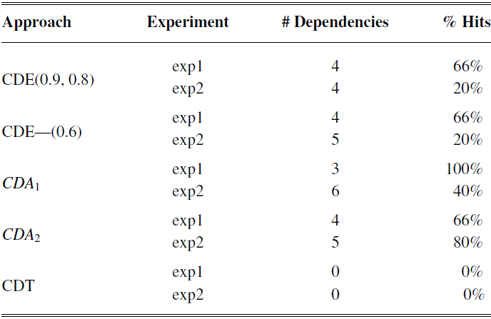
Table 7 confirmed our intuition, showing that with the whole set of individuals CDA1 was able to find all ‘hits’ for Exp1, and even more: it is the only approach able to achieve this. Moreover, the results for Exp2 are also improved. For Exp1, CDA2 has a comparable result to the other approaches, but it is a lot better on Exp2, which might indicate that CDA2 behaves better on more complex terminology learning problems. The results for CDE did not change as much as when the completeness is relaxed. Therefore, when all the individuals are known or when the examples are a more significant sample of the domain, the CDA method seems the better choice. The CDT approach found far less dependencies than its counterparts. Table 8 shows the CDT’s hits.

Table 7

Full completeness over the individuals experiment with the methods CDE, CDA and CDT

Table 8

Full completeness experiment CDT’s hits

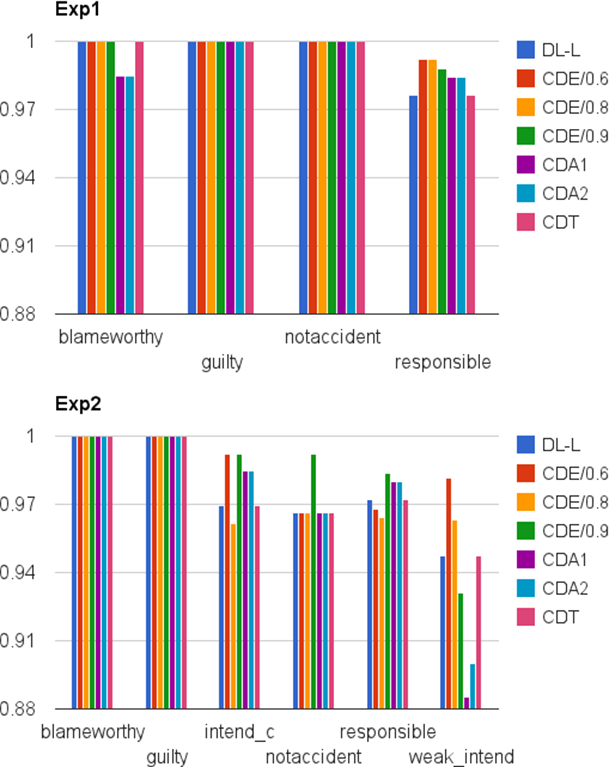
Regarding the analysis of the terminology quality, DL-Learner was also considered. Figure 5 shows the plots of f-measure results for each of the concepts and for all the scenarios. It is possible to notice that all the approaches performed statistically similar in both Exp1 and Exp2, except CDA in Exp2, when inducing the definition of $weak\_intend$ . However, it is important to notice that in this specific case, the appropriate relationships is not considered (see Table 6), possibly because the lack of full completeness due to the 10% of examples reserved for validation, as discussed previously. Therefore, terminology learned with MCL approaches achieve similar predictive results compared to the single concept learning approach. This partially validates the research question Q1: terminologies learned regarding dependencies among the concepts have comparable quality (predictive power) to its counterpart learned with no regard for the dependencies.

Figure 5

F-measure for Exp1 (top) and Exp2 (down) considering scenarios with CDE, CDA, CDT and DL-Learner (DL-L)

Figure 6

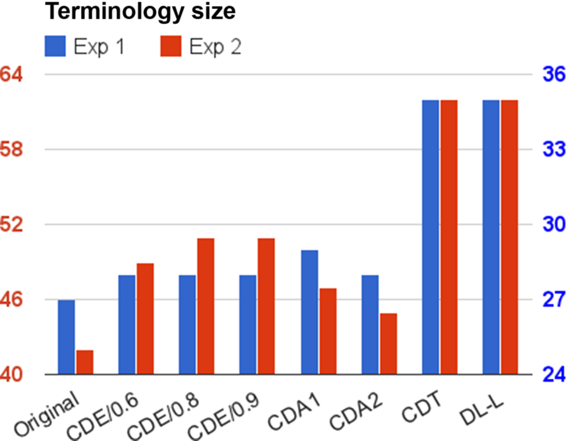
Size of found terminology for Exp1 and Exp2 with methods CDE, CDA, CDT and DL-Learner (DL-L)

Regarding the qualitative metrics, we used the whole set of examples. For the size of the found terminologies, on the far left of Figure 6, we show the original size of the terminology, and none of the approaches achieve results equal or smaller than it. On the far right, we have the size of the terminologies without MCL. None of the approaches produced terminologies larger than it. The CDT results are equal to the DL-Learner’s because no redundancy is found. Apart from CDT, all the proposed methods induced far smaller terminologies than the equivalent concept learning without addressing the dependencies.

In conjunction with the results related to the predictive power, we can conclude that if dependencies among the concept of the domain that need to be learned are found then clearer and concise terminologies are yield while their quality is maintained, successfully answering the research question Q2.

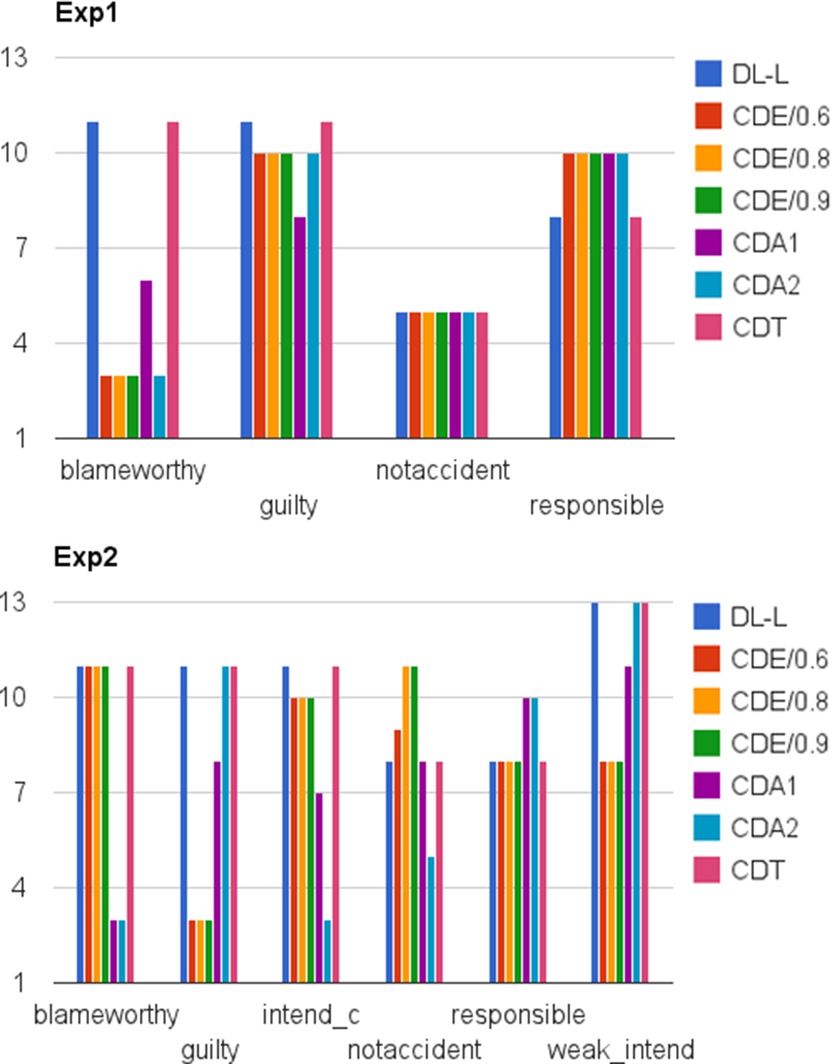
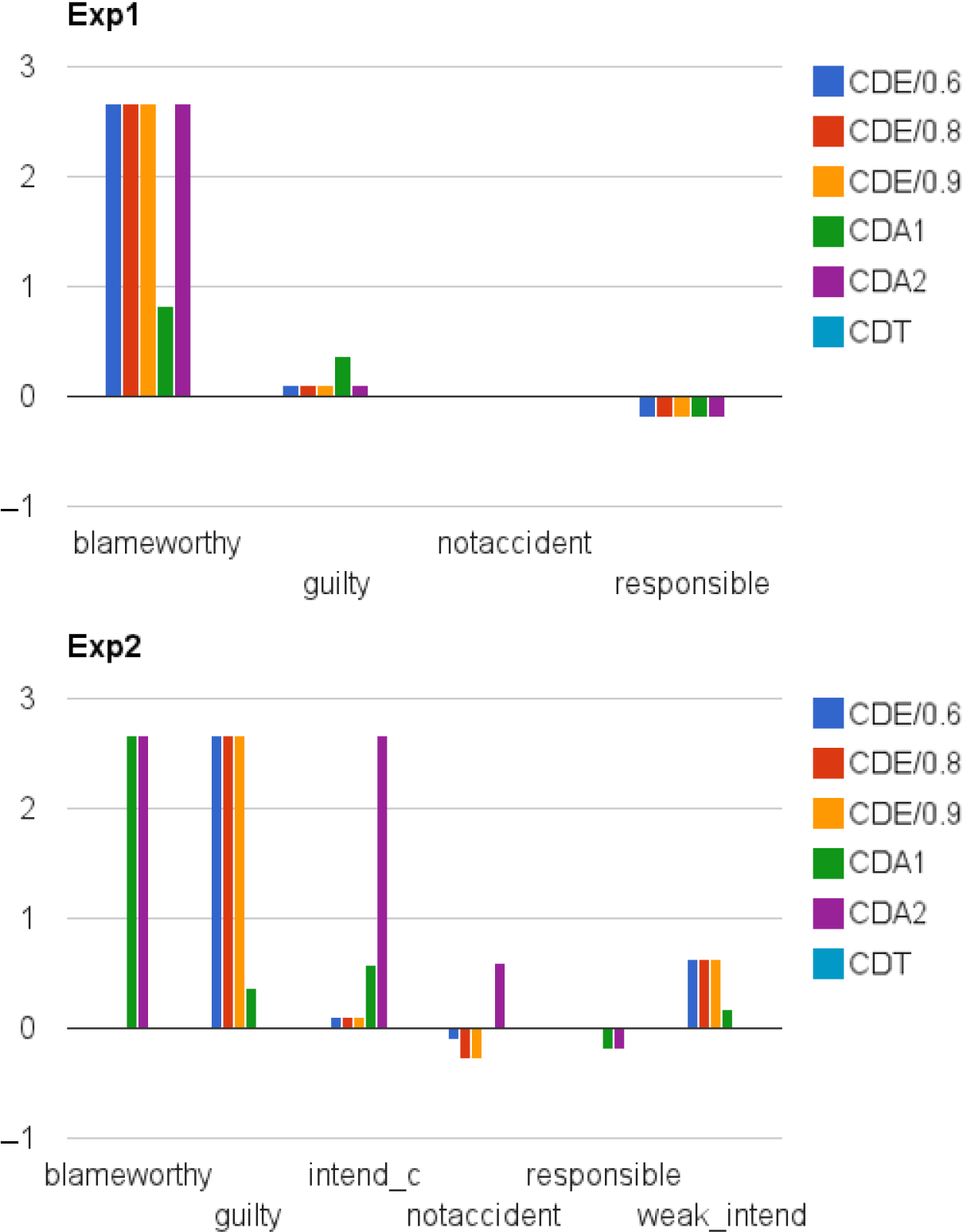
For the size of concept per experiment, see Figure 7. The three CDE strategies have very similar results, consistently better or equivalent to DL-Learner, except on ‘responsible’ in Exp1 and ‘notaccident’ in Exp2. $CDA_1$ has the best result for ‘guilty’ in Exp1, but its ‘blameworthy’ was the worst among our approaches, exp. Interestingly, both CDA found by far the best result for ‘blameworthy’ and ‘intend_c’ in Exp2, with $CDA_2$ being even better, while it is only average in the other results. There is a trade-off on the size of the concepts, as when some instances choose a smaller definition for a concept, the size of other related concepts are affected, because the latter might not be able to use the former. This explains why $CDA_2$ had the best solutions overall, because different from the other approaches it tries alternative definitions for both concepts when a dependency incurs in a cycle.

Figure 7

Size of concepts definitions for Exp1 (top) and Exp2 (down) with methods CDE, CDA, CDT and DL-Learner (DL-L)

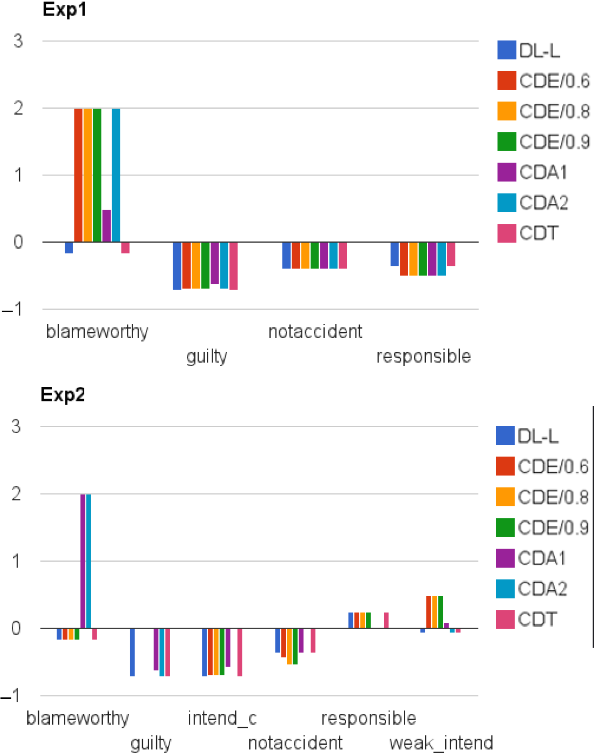
Figure 8 contrasts the size of concepts learned with their original definitions. The values are calculated through the formula $\frac{|original\ definition|}{|learned\ definition|}-1$ , where values over 0 indicates that learned terminology is smaller than the original one. Most of the results were negative, with the size being between 40% to 70% bigger, while some results are positively better as ‘blameworthy’ in Exp1 and ‘responsible’ and ‘weak_intend’ in Exp2, with definitions 200% smaller than the original ones.

Figure 8

Size difference for Exp1 (top) and Exp2 (down) w.r.t. Original Definition with methods CDE, CDA, CDT and DL-Learner (DL-L)

Additionally, a particularly important result is the performance of CDA concerning concept ‘blameworthy’ in Exp2. It provides the higher decrease in size. Due to the fact that CDA uses assertions about all concepts being learned and ‘blameworthy’ is the concept that is most dependent on other concepts from the learning task, it is the one that most benefits from CDA approach. On the other hand, CDE is the worst choice for this concept, since the taxonomy is more complex.

Figure 9 uses the same formula, showing that CDEs and CDAs provide smaller definition than DL-Learner.

Figure 9

Size difference for Exp1 (top) and Exp2 (down) w.r.t. DL-Learner (DL-L) with methods CDE, CDA and CDT

Furthermore, for Exp1 all the definitions learned subsumed the original definitions, while for Exp2 (i) definition for concepts {blameworthy, guilty, responsible} subsumes their original definition when DL-Learner and CDA are performed; (ii) definition for concepts {guilty, intend_c, weak_intend} subsumes their original definition when CDE is performed; (iii) the original definition for {notaccident} subsumes the definition learned with DL-Learner and (iv) the original definition for {notaccident, responsible} subsumes the learned definition when running CDA and CDE.

Summarising, these results show the potential of the MCL approaches proposed in this work, to find smaller more readable solutions and, in some cases, solutions equivalent to those created by human beings. Furthermore, CDE proved to be less susceptible to the completeness assumption, while CDA was very sensible to it. $CDA_2$ displayed a very good performance, being the closest to the original terminology on the more complex experiment (Exp2); however, one must not forget the additional cost of relearning the concepts to remove the cycles. Finally, the CDT approach found far less dependencies than its counterparts. This is due to the fact that syntactical substitutions are far more unlikely when the set of concept learning problems have a wide range of possible solutions. Thus, we can answer the research question Q3, that is, depending on the employed method, we might well have more concise solutions.

5.1 Concept learning with DLs

In this case, we can see related work from three different points of view: (1) previous work regarding MCL in a DLs setting; (2) works related to single concept learning in DLs, as such methods are used to learn the concept definitions once one of the proposed methods is applied and (3) previous work that learn multiple concepts using logic programming as the underlying representation language, in the field of inductive logic programming.

Focusing on the single concept learning task, most work induce terminologies either independently or using an ad hoc order (Iannone et al., Reference Iannone, Palmisano and Fanizzi2007; Fanizzi et al., Reference Fanizzi, d’Amato and Esposito2008; Lehmann, Reference Lehmann2009). These works are necessary to the MCL methods presented here because an integral part of the task involves learning a single concept definitionFootnote ⁷ , which is learned using one of the existing methods. Other previous works focus on divide-to-conquer strategies to learn single concepts by combining partial solutions built either from a subset of the positive and negative examples, or from different data sources (Tran et al., Reference Tran, Dietrich, Guesgen and Marsland2017; Gao et al., Reference Gao, Guirao, Basavanagoud and Wu2018; Konys, Reference Konys2018). In a future work, a study of the underlying bias of this part of the process should be done, because it appears that each method has a slightly different focus, either on the general to specific direction (Fanizzi et al., Reference Fanizzi, d’Amato and Esposito2008; Lehmann & Hitzler, Reference Lehmann and Hitzler2010) or in the specific to general (Iannone et al., Reference Iannone, Palmisano and Fanizzi2007). To that and to better validate our method, we can also leverage recently proposed logical measures to the problem of ontology leaning (Shamsfard & Barforush, Reference Shamsfard and Barforush2003; Barforush & Rahnama, Reference Barforush and Rahnama2012), such as dissimilarity and complexity (Sazonau & Sattler, Reference Sazonau and Sattler2017). YinYang (Iannone et al., Reference Iannone, Palmisano and Fanizzi2007) provides a method that refines definitions after a single concept is learned, which is related to our CDT method. However, while the refinement focuses on a single concept, CDT tries to find dependencies within a whole terminology and refine it, from such dependencies.

Next, with respect to terminology learning considering the induction of a set of related but distinct concepts, to the best of our knowledge, the literature is rather scarce. Previous works have tried to handle this problem by including the human in the loop: in Konev et al. (Reference Konev, Lutz, Ozaki and Wolter2017b), taxonomies containing possibly related concepts are learned by focusing on the communication process between the ontology engineer and a domain expert, while in Sazonau et al. (Reference Sazonau, Sattler and Brown2015) the terminology induction is targeted as a multi-objective problem, where the induced hypotheses are presented to a domain expert to accept or reject them, aiming at quality measures. Here, our three different approaches lean terminologies completely automatically. Another work related to ours conceives the analysis of formal concepts to find out the best way to learn a terminology (Baader et al., Reference Baader, Ganter, Sertkaya and Sattler2007). One seemingly related work is Distel (Reference Distel2011), where definitions for multiple concepts are induced using formal concept analysis concepts. However, this work does not do MCL as described here, it is more in-line with finding the complete set of relationships within a terminology without the use of new examples.

5.2 Multiple predicate learning in ILP

Finally, a large portion of the theoretical background used by concept learning methods in DLs can be traced back to earlier works on the ILP area, specially with regard to some of the basic formalisms. The seminal works (Muggleton, Reference Muggleton1991, Reference Muggleton1992) provide some of the shared formalisms of this method. Although, a big theoretical intersection exists between the two fields, specific implementations are required because of particular idiosyncrasies that emerge from the particular knowledge representation—descriptions logics and logic programming, in concept learning in DL and predicate learning in ILP, respectively.

Although a direct correlation between solutions for ILP and concept learning might not occur, the cross-pollination of ideas is healthy for both areas of research. In De Raedt et al. (Reference De Raedt, Lavrac and Dzeroski1993), the problem of multiple predicate learning is described, the description is very similar to Definition 3. It presents the major drawbacks and some path to solutions for multiple predicate learning. In essence, this work states that learning multiple predicates is more difficult than learning single predicates, as the former is not limited to the generation of several independent predicate definitions but involves the discovery of predicates dependencies. One of the possible solutions for the problem is the proper ordering of the predicate learning tasks, we presented in this paper Section 3.1.2 a method that aims at that. A different solution called MPL is presented, in it the refinement operator used deals with clauses with only the body, assigning a predicate to the head as the last step when evaluating a clause. This allows for evaluating a clause definition apart from a particular predicate. In this instance, the predicates are learned out of order and might contain multiple clauses with other predicates that were also learned in the body. As it is, MPL would not work in the DL setting because one of the basic assumptions is that a concept has only one definition, with some changes this might work within the assumptions, if instead of working with clauses it used hypothesis.

The mechanisms proposed in the literature to solve multiple predicates learning can be separated into approaches that work in the normal ILP with some kind of interleaving learning of clauses (De Raedt et al., Reference De Raedt, Lavrac and Dzeroski1993) setting or approaches that use an alternative setting to minimise some of the problems (De Raedt & Lavrač Reference De Raedt and Lavrač1996; Muggleton & Bryant, Reference Muggleton and Bryant2000). These types of solutions cannot be directly applied to the problem in DL because in logic programming a predicate (concept) can be defined by several clauses, while in DL a concept (predicate) can have at most one definition. Bratko (Reference Bratko, Dzeroski and Flach1999) presents an ad hoc method that have profound similarities with DL, and it generates full hypothesis instead of doing one clause of a time.

5.3 Multitask and curriculum learning

In a more general point of view, the algorithms developed here are related to the multitask learning area (Caruana, Reference Caruana1997), which also focuses on jointly learning multiple related tasks, with a number of successful applications (Liu et al., Reference Liu, Nie, Han, Zhang and Rosenblum2015, Reference Liu, Zheng, Liang, Liu and Rosenblum2016). Thus, in case, one models such tasks using a concept learning setting, the algorithms developed here could also be applied to tackle the same type of problems handled by that area.

In addition, there is a constant effort on characterising and developing curriculum learning algorithms, so that machines would learn in an organised way (Bengio et al., Reference Bengio, Louradour, Collobert and Weston2009; Jiang et al., Reference Jiang, Meng, Zhao, Shan and Hauptmann2015). To achieve that, different concepts could be introduced at different times, in the same way that most of human educational systems work. The basic idea is to start from easier tasks and gradually moving on to the more difficult ones. The algorithms developed here aim at this same strategy, however addressing concept learning in a DL setting.