Introduction
The McMurdo Dry Valleys of southern Victoria Land comprise a predominantly ice-free region within the Transantarctic Mountains (Fig. 1). On average, the region receives < 10 cm of annual precipitation (Schwerdtfeger 1984) and mean annual temperatures range from -30° to -15°C (Doran et al. Reference Doran, McKay, Clow, Dana, Fountain, Nylen and Lyons2002). On the basis of mapped geomorphic features and spatial variations in modern soil moisture and atmospheric temperature, the region can be divided into a series of microclimate zones. Beacon Valley (77°51′S, 160°35′E, Fig. 1) is the largest valley within the stable upland microclimate zone, the coldest and driest zone as mapped by Marchant & Denton (Reference Marchant and Denton1996) and Marchant & Head (in press). The valley has received significant attention since the documentation of massive subsurface ice (Linkletter et al. Reference Linkletter, Bockheim and Ugolini1973, Potter & Wilson Reference Potter and Wilson1984), some of which is related to southward incursions of an ancestral Taylor Glacier and may be of Miocene age (Sugden et al. Reference Sugden, Marchant, Potter, Souchez, Denton, Swisher and Tison1995).
Topography of Beacon Valley, Antarctica. Hillshade generated from high-resolution LiDAR DEM (collected as a joint effort by NSF/NASA/USGS with processing by Schenck et al. (2004)) embedded in 30 m resolution DEM of the entire McMurdo Dry Valleys region derived from stereo data (available from the US Antarctic Resource Center). The boundary between these two datasets is visible at the abrupt change in resolution around the margins of the Beacon valleys tributaries. The debris-covered glaciers in Mullins and Friedman Valley are labelled. White outline shows the location of Fig. 2.

An additional source for some of the buried ice in upper and central Beacon Valley is debris-covered glaciers that originate from cirques in tributary valleys of upper Beacon Valley (Fig. 1). The Mullins Valley debris-covered glacier (Figs 1 & 2) and the smaller Friedman Valley debris-covered glacier (Fig. 1) both grade from small, exposed alpine glaciers, covered only by a scattering of dolerite cobbles and boulders, to buried glacial ice that extends several kilometres downvalley. These features contain a demonstrable core of glacier ice, which we feel distinguishes them from most “rock glaciers” that typically, in whole or in part, consist of debris mobilized by flow of interstitial ice of secondary origin. The glacier ice in Mullins and Friedman valleys is capped by sublimation till, produced primarily as englacial debris is brought to the surface via sublimation of overlying ice (Schaefer et al. Reference Schaefer, Baur, Wieler, Denton, Ivy-Ochs, Schluchter and Marchant2000, Marchant et al. Reference Marchant, Lewis, Phillips, Moore, Souchez, Denton, Sugden, Potter and Landis2002). The surface topography of these debris-covered glaciers is marked by a series of ~1–6 m high arcuate ridges and furrows (Figs 1 & 2). The ridges are cored by glacier ice and there is little change in the thickness of overlying till, suggesting that ridge morphology is related to compression or thrusting of subsurface ice rather than to localized variations in the sublimation till.
Aerial photo of the debris-covered glacier within Mullins Valley (USGS TMA3080-F32V-275). Note the continuous debris cover and arcuate ridge and furrow pattern on the surface of the glacier downvalley of the superposed meltwater ice (near UMT). Thick black lines show the locations of seismic lines, with triangles representing the location of the 12-geophone spread and asterisks representing maximum offsets for forward and reverse line orientations. The lines are labelled according to their location and orientation, UM = Upper Mullins site, CM = Central Mullins site, LM = Lower Mullins site, with L = Longitudinal Survey, and T = Transverse Survey. Dashed white lines represent location of cross-sectional DEM profiles in Fig. 3. Solid white line approximately along the centreline of Mullins Valley shows location of the continuous ice thickness profile in Fig. 8. Tick marks with labels are located every 0.5 km. The coarse nature of this line is due to the grid spacing of the InSAR data from Rignot et al. (Reference Rignot, Hallet and Fountain2002).

Solar radiation during summer months warms low albedo (0.07) dolerite rocks above 0°C. Where these isolated rocks occur scattered across a relatively clean ice surface, such as near valley heads, meltwater forms and flows down local slopes. Although most of this meltwater evaporates, some flows tens of metres before refreezing as superposed ice just inside the first major topographic ridge on both the Friedman and Mullins valleys debris-covered glaciers (Figs 1 & 2). Beyond the first few ridges, the sublimation tills are sufficiently thick (> 10–50 cm) to prevent melting at the buried ice surface; ice loss in these regions is entirely by sublimation, with maximum rates likely reaching ~0.1 mm yr-1 (Kowalewski et al. Reference Kowalewski, Marchant, Levy and Head2006). As reported in Levy et al. (Reference Levy, Head and Marchant2006), thermal-contraction polygons mark the surface of these sublimation tills and show progressive downvalley changes in size, orientation, and maturity.
Details of the Mullins Valley debris covered glacier
The Mullins Valley debris-covered glacier ranges from approximately 500 m to 800 m wide. It occupies the length of Mullins Valley and displays a notable, north-east bend at the entrance to Beacon Valley proper (Figs 1 & 2). Beyond this bend, the arcuate, ridge-and-furrow surface morphology diminishes progressively, the style of polygons marking the till surface changes from oriented to non-oriented (Levy et al. Reference Levy, Head and Marchant2006), and the till thickness increases to its maximum values of ~75–100 cm.
The till is derived from rockfall at the head of Mullins Valley. Ferrar Dolerite, Beacon Heights Orthoquartzite, and other members of the Beacon Supergroup comprise the main lithologies observed in the sublimation till and in shallow ice cores (~5 m depth), all of which are exposed as bedrock along cliff faces above the ice accumulation zone at the head of Mullins Valley. Most of these clasts travel englacially before they are brought to the surface as the overlying ice sublimes; however, a few clasts fall directly on the ice ablation zone and in these cases, transport is entirely supraglacial. Subglacial debris entrainment mechanisms such as pressure-melting and regelation are unlikely for the Mullins Valley debris-covered glacier due to 1) the low ice temperatures (mean annual temperature at 10 m depth is -26°C, Kowalewski, personal communication 2007), 2) the relatively thin ice thickness measurements presented in this work, and 3) the slow horizontal ice velocities (≤40 mm a-1), as reported in Rignot et al. (Reference Rignot, Hallet and Fountain2002).
The lateral margins of the Mullins Valley debris-covered glacier are often characterized by collections of cobbles and boulders near the angle of repose, with a relief of ~1–5 m (see fig. 3 in Lorrey Reference Lorrey2005). However, the northern limit of the Mullins Valley debris-covered glacier in central Beacon Valley is diffuse (Fig. 2), and a distinct morphologic break is not observed at the surface. At depth, the ice most likely abuts, in an unknown fashion, buried ice from an ancestral Taylor Glacier first described in Sugden et al. (Reference Sugden, Marchant, Potter, Souchez, Denton, Swisher and Tison1995) and later in Marchant et al. (Reference Marchant, Lewis, Phillips, Moore, Souchez, Denton, Sugden, Potter and Landis2002). Our inferred limit of the Mullins Valley ice is based on the map pattern and lithology of granite-bearing (Taylor Glacier provenance) and non-granite bearing (upper Beacon Valley provenance) sublimation tills that rest on buried ice in central Beacon Valley (Moore Reference Moore2002). Though active horizontal ice flow is largely restricted to the upper ~3.5 km of the Mullins Valley debris-covered glacier (Rignot et al. Reference Rignot, Hallet and Fountain2002), a conservative estimate for the full length of the glacier is at least ~7 km, with the last 2+ km of the glacier essentially stagnant.
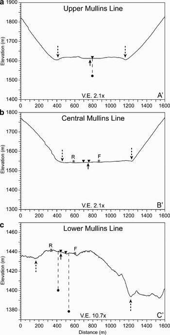
Cross-sectional topographic profiles extracted from LIDAR DEM across each of the survey sites. Upward-pointing solid arrows show intersection of the ice thickness profile in Fig. 8, long dashed lines with arrows show margins of the debris-covered glacier, downward pointing triangles show location of geophone spread, asterisks show maximum source offsets for forward (F) and reverse (R) orientations, and solid circles with dashed lines indicate ice thickness estimates from seismic reflections. a. Profile across superposed meltwater ice at the Upper Mullins Transverse Line. Note the general convex-upward shape of the glacier surface at this location. The downward-pointing triangle represents the location of the Upper Mullins Longitudinal Line with ~90 m ice thickness estimate. b. Profile across the Central Mullins Transverse Line. c. Profile across Lower Mullins Transverse Line. Note the significantly higher vertical exaggeration (10.7x) for this profile and the lack of steep valley walls on either side of the debris-covered glacier. Ice thickness estimates plotted for reverse (~40–45 m) and forward (~60–65 m) shots at their respective midpoints. All elevation data given as height above WGS 1984 geoid.

The occurrence of near-surface glacier ice in Beacon Valley has been known for decades (Linkletter et al. Reference Linkletter, Bockheim and Ugolini1973, Potter & Wilson Reference Potter and Wilson1984), but its depth, age, and source(s) are poorly constrained and are the subject of current debate (Ng et al. Reference Ng, Hallet, Sletten and Stone2005). Given this debate, as well as the fact that debris-covered glaciers have the potential to store long-term climate records (Clark et al. Reference Clark, Steig, Potter, Fitzpatrick, Updike and Clark1996, Steig et al. Reference Steig, Fitzpatrick, Potter and Clark1998, Konrad et al. Reference Konrad, Humphrey, Steig, Clark, Potter and Pfeffer1999) and serve as terrestrial analogues for features interpreted as debris-covered glaciers on Mars (Head & Marchant Reference Head and Marchant2003, Head et al. Reference Head, Hiesinger, Kreslavsky, Milkovich, Neukum, Werner, Van Gasse, Jaumann, Hauber, Hoffmann, Carr, Masson and Foing2005, Shean et al. Reference Shean, Head and Marchant2005, Reference Shean, Head, Marchant and Fastook2007, Milkovich et al. Reference Milkovich, Head and Marchant2006), we re-examine the Mullins Valley debris-covered glacier to refine estimates for its ice thickness and debris content and to set the stage for detailed analyses of ice cores from this glacier.
Prior estimates of ice thickness
As a first step towards understanding the ice dynamics within this system, Rignot et al. (Reference Rignot, Hallet and Fountain2002) utilized synthetic aperture radar interferometry (InSAR) to measure surface displacement over a 3.3 year period (1996–1999) for the Mullins Valley debris-covered glacier. From these data they estimated maximum horizontal surface velocities of ~40 mm yr-1 near the valley head to “vanishingly small” velocities (< 1 mm yr-1, approaching error estimates) on the floor of central Beacon Valley. Given the surface slope of the glacier and these horizontal velocity estimates, they derived preliminary ice thickness estimates of ~20 to > 80 m (fig. 3 from Rignot et al. Reference Rignot, Hallet and Fountain2002).
Survey descriptions and data collection
In November 2004, we completed six shallow seismic reflection surveys along the Mullins Valley debris-covered glacier. Data were collected for a minimum of two lines at each of the three major survey sites (termed Upper, Central, and Lower); lines parallel to the valley centreline are designated “longitudinal”, and those perpendicular, “transverse” (Fig. 2). All surveys were completed using a 12-channel Geometrics Geode seismograph with 14 Hz, vertical geophones. The geophone spacing for these surveys was 5 m with a sampling interval of 1/16 ms.
In locations where the ice was not directly accessible, the sublimation till was removed to expose the underlying glacial ice. A tapered drill bit was used to drill pilot holes in the ice and the geophones were set firmly into these holes, where they froze into place. The geophone and takeout cables were then secured with stakes and surface rocks to minimize noise from wind.
Based on shallow reflection survey results reported for Matanuska Glacier (Baker et al. Reference Baker, Pyke, Strasser, Evenson, Lawson and Bigl2003) and previous estimates for ice thicknesses in Mullins Valley (Rignot et al. Reference Rignot, Hallet and Fountain2002), we concluded that a sledgehammer source would be sufficient to image the ice/bedrock interface. Thus, the source for all shots was a 5.45 kg (12 lb.) sledgehammer struck on a 20 × 20 cm aluminium plate set directly on the glacier surface. We employed a source-moveout survey design, with a stationary geophone array and a moving source repositioned at 0, 5, 30, 60, 90 and 105 m offsets along the axis of the geophone array. Each line was shot in both forward and reverse orientation with an additional shotpoint located in the centre of the geophone array. Typically, data were recorded for individual shots and then as stacks of 5, 10, 15 and 20 shots. Due to the preponderance of surface irregularities (polygon furrows, boulders, sand-wedges truncating near surface ice), the locations of some geophones and/or shotpoints were offset from prescribed intervals by 10–20 cm with only a few offset by > 20 cm.
Data processing
All data were processed with the open source SeisUnix software package developed by the Center for Wave Phenomena at the Colorado School of Mines (Stockwell Reference Stockwell1999). For each line, the data collected for all source offsets were combined to produce common offset stacks (pseudowalkaway plots), allowing for analysis of the entire line in one plot (see Fig. 5). The processing flow for these plots included the following steps: 1) bad trace removal, 2) trace offset correction (position and time), 3) filtering (typically bandpass w/ linear taper), 4) stacking by offset, 5) gain adjustment, 6) windowing (time), and 7) muting. This method assumes that the subsurface velocities are laterally homogeneous and vertically layered relative to the surface (Vincent et al. Reference Vincent, Steeples, Tsoflias and Sloan2005).
Although the survey design only provided a ~2–3 trace fold, common midpoint plots were produced to complement the pseudowalkaway plots. The processing flow for the common midpoint plots was similar to that for the common offset stacks. After filtering, the data were: 1) muted to remove ground roll, 2) corrected for normal move-out (NMO), 3) sorted by common midpoint, 4) stacked by common midpoint (~2–3 trace fold), 5) scaled, and 6) windowed. For each line, a range of possible NMO velocities were tested before a final NMO correction was applied. This effectively corrected traces with non-zero offsets for the additional traveltime from source to receiver using the given NMO velocity, resulting in a plot where the reflector is shown as if both the source and receiver were directly above the reflection point for the entire profile.
The frequency content of each line was unique despite the fact that the same hammer source was used for all surveys. This may be attributed to different team members swinging the hammer on different days and/or to the nature of the surface beneath the plate at each site. As a result, customized filters were applied to data from each line during processing and analysis. In most cases, the frequency content of the surface waves (ground roll) was similar to that of the direct waves and reflected arrivals, rendering most attempts to remove ground roll unsuccessful. This factor combined with the low fold number (~2–3) reduced the coverage of common-midpoint plots.
Results and discussion
As described below, two of the surveys on the debris-covered glacier within Mullins Valley show clear reflections interpreted to represent the ice/bedrock interface. These reflections are visible at large source offset distances, where pulse-like, high-amplitude ground roll arrives well after the reflected phases. After the ground-roll arrivals, all traces are dominated by low frequency, high amplitude arrivals that obscure later arrivals, despite several filtering attempts.
Upper Mullins longitudinal line
This survey was performed parallel to the centreline of the debris-covered glacier (Figs 2–4). The geophone array was located at the head of Mullins Valley in a region with little surface debris, such that all forward shotpoints were situated on the superposed meltwater ice and all reverse shots were located on exposed glacial ice farther upvalley (Figs 2 & 4).
a. Context photograph of the Upper Mullins Longitudinal Line, looking upvalley (in direction of reverse shots) from the edge of the superposed meltwater ice. The geophone spread is oriented along the tape in the centre of the image running approximately along the valley centreline. Note the exposed glacial ice between dolerite cobbles and boulders from rockfall along the cliffs surrounding the accumulation zone of the glacier. b. Context photograph of the Lower Mullins site, looking north-east (in direction of forward shots) towards Taylor Glacier. Note the continuous debris cover with large boulders (some > 1–1.5 m across) and relatively uneven surface. White arrow points to person for scale.

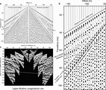
Analysis of the common offset stack (Fig. 5), produced with high shot stack numbers (n = 15) at offsets > 60 m, reveals four distinct phases. These include the direct wave (~3800 m s-1), a reflected phase with intercept at ~47 ms (forward) and ~51 ms (reverse), and an S-wave phase (~2000 m s-1) that splits from the ground roll phase (~1850 m s-1) at larger offsets due to its higher velocity (Fig. 5). The measured P-wave velocity, S-wave velocity, and VP/VS of these data are consistent with previous estimates for pure ice (Kohnen Reference Kohnen1974, Lee et al. Reference Lee, Hutchinson, Collett and Dillon1996).
a. Common offset stack for Upper Mullins Longitudinal Line after a 100–650 Hz bandpass filter with 100 Hz linear taper, 3 ms window AGC, and clipping at 95%. Arrows highlight the reflected phases on both the forward and reverse lines. b. Annotated sub-section of common offset stack for large forward offsets. c. Common midpoint plot with depth plotted for a NMO velocity of 3800 m s-1. Position on reflector is relative to the zero for forward shots. Dashed line shows interpreted reflector depth across the length of the profile ranging from ~88–97 m with greater depths upvalley.

After normal move-out (NMO) correction for a velocity of 3800 m s-1, the reflected phase yields a depth of ~88 m for the forward shots and ~97 m for the reverse shots. The common midpoint plot (Fig. 5) shows the depth at different locations on the surface of the reflector. The reflector appears relatively flat, with a slight downward dip upvalley. We interpret the reflected arrivals observed in both forward and reverse shots to represent the interface between the glacial ice and bedrock (most likely sandstone or dolerite). These depth estimates for the ice/bedrock interface agree with previous estimates from ice flow modelling (Rignot et al. Reference Rignot, Hallet and Fountain2002) and with valley wall extrapolation in cross-sectional profiles for a typical U-shaped glacial valley (Fig. 3). We cannot distinguish any layering within the ice at this location based on these initial data.
The depth estimates for the Upper Mullins Longitudinal Line are of high-confidence based on the strength and coherence of the observed reflected phase, the observation of similar reflections in both forward and reverse orientations, and a best-fit NMO velocity consistent with relatively cold, pure ice (3800 m s-1). These data confirm that the debris-covered glacier within Mullins Valley contains a ~90–95 m thick homogeneous layer of pure ice above a coherent reflector at this location.
Lower Mullins transverse line
The Lower Mullins survey site was located where the Mullins Valley debris-covered glacier enters Beacon Valley proper (Fig. 2). Surface conditions at this location are very different from the relatively clean, exposed glacial ice and superposed frozen meltwater ice at the Upper Mullins site. The sublimation till at this site is ~40 cm thick and large dolerite boulders are present at the till surface (Fig. 4). Sublimation-type polygons are widespread, and the troughs delineating such polygons approach a depth of ~1 m (Levy et al. Reference Levy, Head and Marchant2006).
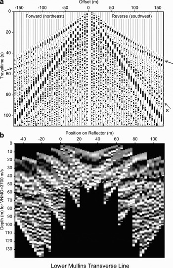
The common offset stack for the transverse line at the Lower Mullins site shows reflected phases in both forward and reverse shots (Fig. 6). The forward shots were oriented to the north-east of the geophone array, closer to the actual centreline of Mullins Valley (Figs 2–4). The best fit for the direct wave arrivals in the forward shots corresponds to a P-wave velocity of ~3640 m s-1. An apparent reflected phase is observed at large source offsets (90, 105 m) for the forward shots (left side of Fig. 6). For a best-fit NMO velocity of 3700 m s-1, this phase has an intercept of ~33 ms, yielding depth estimates of ~60–65 m.
a. Common offset stack for Lower Mullins Transverse Line with a 700 Hz highpass filter with 100 Hz linear taper and clipping at 85%. Solid arrows highlight the reflected phases on both the forward and reverse lines. Dashed arrow highlights the S-wave phase observed for the reverse shots with a velocity of ~1950 m s-1. b. Common midpoint plot with depth plotted for a NMO velocity of 3700 m s-1. Position on reflector is relative to zero for forward shots. Dashed line shows interpreted reflector depth across the length of the profile ranging from ~40 m in reverse shots and ~60–65 m in forward shots. This northward dip is consistent with the dip of the western wall of Mullins Valley.

A higher amplitude, shallower phase is observed for the reverse shots (right side of Fig. 6), with an intercept of ~23 ms for an NMO velocity of 3700 m s-1. This shallow phase in the reverse shots may represent reflected arrivals, refracted arrivals, or a combination of the two. Based on the observed arrival times, velocities, and the survey geometry, the reflected and refracted phases should arrive at approximately the same time, with a crossover distance of ~95–105 m. If these arrivals represent a reflected phase, then depth estimates of ~40–45 m are obtained. Alternatively, if the phase represents a refraction, then the velocity obtained for the lower layer (bedrock beneath an ice layer with a velocity of ~3700 m s-1) is approximately ~5300 m s-1, which is consistent with fractured basalt (Burger Reference Burger1992). Extrapolation of the bedrock stratigraphy exposed in the valley walls suggests that the bed beneath the ice should be Ferrar Dolerite, a fractured intrusive sill of mafic composition (Fig. 2). For this velocity structure, the arrival times of the potential refracted phase give depth estimates of ~40 m, similar to the depth predicted for the reflected phase. Thus, we interpret the available data to suggest that the depth to bedrock is ~40–45 m beneath the reverse shots.
On the basis of these depth estimates, (~60–65 m for the forward shots and ~40–45 for the reverse shots), it appears that the reflector at the lower Mullins Transverse Line is dipping ~10°N, which is not an ideal configuration for a pseudowalkaway plot. With this in mind, we produced a common midpoint plot (CMP, for an NMO velocity of 3700 m s-1), assuming that both phases are reflections from the same interface (Fig. 6). The CMP suggests that the interface shows a general increase in depth from the south-west to the north-east (Figs 2 & 6).
Unlike the case for the Upper Mullins Longitudinal Line, the difference between modelled depths for the forward (~60–65 m) and reverse (~40–45) shots on the Lower Mullins Transverse Line is significant. In order to understand this disparity, we considered the location of this line with respect to the valley walls (Figs 1–3). Figure 2 shows that the reverse shots are relatively close to the western wall of Mullins Valley, whereas the shots on the forward line are at considerably greater distances from the valley wall. Thus, the shallower bed depths inferred for the reverse shots (closer to the western wall) would be expected. In addition, the Lower Mullins survey site is situated near the location where the debris-covered glacier makes a distinct northward turn as it enters Beacon Valley (Figs 1 & 2). This notable change in flow direction may have originated due to interactions with the Friedman Valley debris-covered glacier (Fig. 1), bedrock control, or some combination of the two. The relatively steep bedslope of ~10°N inferred from the common-midpoint plot is consistent with reasonable estimates of sub-ice topography beneath the Lower Mullins Site (Fig. 3).
Central Mullins
We conducted additional shallow seismic surveys at the Central Mullins site (Fig. 2). Although the data are generally of lower quality, a potential reflected phase may be present at ~65 m, but the results are inconclusive.
P-wave velocity variation and ice properties
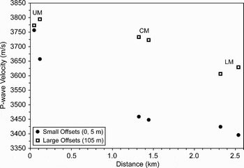
In addition to the estimates of ice thicknesses obtained from reflected arrivals, we can obtain information about the nature of the ice through P-wave velocity analysis. At each line, P-wave velocities were extracted from direct wave arrivals in unstacked data for large-distance (105 m) and small-distance (0 or 5 m) source offsets. Measurements from the forward and reverse shots at each line were similar, and the values plotted in Fig. 7 represent averages for forward/reverse measurements.
Plot of P-wave velocities (extracted from direct wave arrivals) for the two lines at each survey site (UM = Upper Mullins, CM = Central Mullins, LM = Lower Mullins). Note the large velocity difference (~200–300 m s-1) between small (solid circles) and large (open squares) source offsets at the Central and Lower Mullins sites, suggesting the presence of faster ice at greater depths for these sites. Also note the general decrease in velocity for both small and large source offsets with increasing distance along the glacier within Mullins Valley, suggesting that the nature of the ice is changing with distance downvalley.

The first result is the noticeable difference in the P-wave velocity when comparing the small versus large offsets, (note especially Central and Lower Mullins sites; Fig. 7). This suggests that the larger-distance offsets are sampling faster ice at greater depths (more than a few metres) and that the shorter-distance offsets are sampling a thin layer of near-surface ice with slower velocities. The slower near-surface velocities at the central and lower Mullins sites may arise from 1) variations in ice-surface morphology (e.g. polygons), 2) open air cracks at polygon troughs, 3) debris-filled cracks situated at polygon troughs and scattered across the glacier surface (Levy et al. Reference Levy, Head and Marchant2006), 4) warmer near-surface ice temperatures (e.g. Kohnen Reference Kohnen1974), or some combination of these factors. At the Upper Mullins site, the similarity between the velocity measurements (Fig. 7) suggests that relatively uniform ice conditions are present, with minimal open-air or debris-filled cracks near the surface; an assertion that is consistent with visual inspection of shallow ice cores (~10 m) at this location.
In addition to the velocity difference observed for small and large offsets (sampling shallow and deeper ice, respectively), the results show a general decrease in all velocity measurements downglacier (Fig. 7). We interpret this decrease as a result of the greater concentration of open-air or debris-filled cracks with distance downvalley (Lorrey Reference Lorrey2005, Levy et al. Reference Levy, Head and Marchant2006). This general velocity decrease may also be related to a change in the material properties of the ice, which could be the result of greater debris content downvalley, a conclusion that is consistent with visual inspection of near-surface ice and shallow ice cores (~5 m deep) along the length of the Mullins Valley debris-covered glacier.
Ice thickness profiles
Using surface velocities derived from ERS-1/ERS-2 InSAR and surface topography from a USGS 30 m resolution Digital Elevation Model (DEM), Rignot et al. (Reference Rignot, Hallet and Fountain2002) calculated ice thickness for a flow line oriented approximately along the centreline of the Mullins Valley debris-covered glacier (see Fig. 2 for profile location). After Konrad et al. (Reference Konrad, Humphrey, Steig, Clark, Potter and Pfeffer1999), the ice thickness, h, at any position along a flowline can be estimated using:

assuming mass conservation (very small sublimation, e.g. Kowalewski et al. Reference Kowalewski, Marchant, Levy and Head2006) and no basal sliding where u is the surface velocity, n is the flow exponent, ρ is ice density (917 kg m-3), α is surface slope, g is the acceleration of gravity, and A is the flow parameter (ice hardness). We ignore the negligible mass contribution of the sublimation till (< 100 cm thick).
The flow parameter
We can use the observed thicknesses from our seismic surveys, to constrain estimates for the flow parameter, A. Rearranging Eq. (1) (assuming n = 3.0), we obtain a value for A of 2.34 × 10⁻²⁴ s-1Pa-1/3 for the Upper Mullins Longitudinal Line (h = 92), and 1.27 × 10⁻²⁵ s-1Pa-1/3 for the Lower Mullins Transverse Line (h = 40, where the flowline intersects the transverse line). These values for A are consistent with the calculated value of 1.36 × 10⁻²⁴ s-1Pa-1/3 for pure ice at -23°C, the mean annual temperature in Beacon Valley proper (Rignot et al. Reference Rignot, Hallet and Fountain2002).
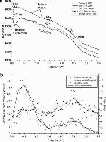
As noted above, the reduction in P-wave velocity with distance downglacier suggests a change in the material properties of the ice. As a result, values for A should change downglacier as well. While Rignot et al. (Reference Rignot, Hallet and Fountain2002) used a constant A, we assume that the flow parameter values calculated from seismic thicknesses are good estimates for the ice at their respective locations. We compute a linear fit between these two values (2.34 × 10⁻²⁴ s-1Pa-1/3 at the Upper Mullins site and 1.27 × 10⁻²⁵ s-1Pa-1/3 at the Lower Mullins site), with a constant A for all distances beyond the Lower Mullins Transverse line to avoid negative estimates for A. Using Eq. (1), we plot two ice thickness profiles - one using this variable A technique and the other for a constant value of A (2.34 × 10⁻²⁴ s-1Pa-1/3) assumed along the entire flowline (Fig. 8).
a. Profile along the centreline of Mullins Valley (as defined by Rignot et al. (Reference Rignot, Hallet and Fountain2002)), see Fig. 2 for context. Upper surface (grey line) is topography extracted from LiDAR DEM with two predicted bed surfaces shown, one for a constant flow parameter calibrated using the ~92 m ice thickness from the Upper Mullins Longitudinal Line (dashed line) and the other using a variable flow parameter calibrated to both the ~92 m thickness at the Upper Mullins Longitudinal Line and the ~40 m thickness at the Lower Mullins Transverse Line (solid line, see text). The locations of the three longitudinal lines are plotted on the surface with asterisks representing 105 m shot offsets and downward pointing triangles representing geophone spreads. The intersections of the transverse lines with the profile are shown with upward pointing arrows and the dashed lines with solid circles represent seismic ice thickness estimates. Note the surface ridges and the bedrock depression beneath the Upper Mullins Site. b. Plot of horizontal velocity (open circles) and slope data (crosses) with smoothed fits used as inputs for Eq. 1. Unfortunately, the Upper Mullins site is located within ~60 m of the beginning of the velocity profile extracted by Rignot et al. (Reference Rignot, Hallet and Fountain2002) (Fig. 2), where velocities are less accurate and large data gaps exist within the interferogram, reducing the quality of ice thickness estimates in these regions. In addition, the three points at distances of ~110–160 m along the profile are located on the flat, superposed meltwater ice bounded by the first ridge at the head of the glacier (Fig. 2). The flat slopes calculated for these three points are not representative of the actual glacial surface, yielding anomalously fast horizontal velocities, and anomalously large ice thickness estimates. Several attempts were made to account for this anomaly, including the use of multiple smoothing algorithms with windows ranging from ~150–400 m; however, we found that simply removing these three points provided the best results. No matter which smoothing approach is utilized (both with or without the lake surface points), we observe large ice thicknesses beneath the Upper Mullins site that decrease just downvalley of the first surface ridge.

As shown in Fig. 8, ice thicknesses predicted for the two definitions of the flow parameter, A, begin to diverge near the valley head. For the profile calculated with a constant A (calibrated only to the Upper Mullins seismic thickness), predicted ice thickness decreases from ~50–60 m just beyond the upper Mullins site to ~20 m near the Lower Mullins site. In contrast, ice thicknesses prescribed using a variable A suggest an ice thickness near the lower Mullins site of ~40 m, consistent with direct measurements from our seismic data. The good fit at the Lower Mullins site is expected based on the calibration scheme, but by utilizing a changing flow parameter we also produce a realistic and relatively constant ice thickness averaging ~40–50 m for most of the glacier (Fig. 8). These results suggest that modelling efforts using a variable flow parameter, A, provide better estimates of ice thicknesses than those employing a constant flow parameter for the Mullins Valley debris-covered glacier. Additional measurements for ice thickness along the profile will help to better constrain how A varies with position along the glacier.
Updated DEM's, smoothing efforts, and flow exponent considerations
To produce more accurate estimates for ice thickness along the centreline of Mullins Valley, we incorporated new topographic data (2 m spatial resolution DEM for Beacon and Mullins valleys derived from LiDAR data with ~0.1–0.2 m vertical accuracy (Schenk et al. Reference Schenk, Csatho, Ahn, Yoon, Shin and Huh2004)) into our profile. Surface slopes derived from this 2 m DEM, and published horizontal-ice velocity data (from Rignot et al. Reference Rignot, Hallet and Fountain2002) were both smoothed using a moving average function with a ~300 m window. These smoothed data were input into Eq. (1) (with the two definitions of A) to yield the continuous ice-thickness profiles in Fig. 8.
In producing these ice thickness profiles, we also considered the effect of variable flow exponents, using both n = 3 and n = 1.8. The value of n = 1.8 was included based on the results of recent laboratory studies that show that under the low stress and low temperature conditions present in Mullins Valley, grain-boundary sliding becomes the rate-controlling creep mechanism for ice flow (Goldsby & Kohlstedt Reference Goldsby and Kohlstedt2001). However, for the measured surface slopes and horizontal ice velocities (from Rignot et al. Reference Rignot, Hallet and Fountain2002), ice thickness estimates for n = 3 and n = 1.8 are generally similar. The largest differences are observed where velocities are highest (at distances of ~0.2–1.0 km, Fig. 8), with predicted ice thicknesses using n = 1.8 of ~15–20% greater than those predicted for n = 3.0. Differences also occur where velocities approach zero (at distances of ~2.9–3.5+ km), with the predicted ice thicknesses for n = 1.8 being approximately ~10–20% lower than for the case with n = 3.0. However, the two curves are almost identical at all other locations, and in Fig. 8 we only plot estimated bed depths for n = 3.0.
Synthesis
One important result of the profiles presented here is the prediction of large ice thicknesses near the head of Mullins Valley. While this may appear anomalous upon first inspection, the large thickness estimates are directly related to decreasing surface slopes and increasing velocities at these locations (Fig. 8). Although the actual magnitude and shape of this variation are not well constrained, the data strongly suggest that a bedrock depression exists just beyond the headwall of Mullins Valley. This depression may reflect glacial erosion (e.g. cirque formation) beneath an ancestral, wet-based alpine glacier under warmer climate conditions.
The downvalley transition from this predicted bedrock depression to shallower bedrock depths, in conjunction with decreasing ice-surface slopes and increasing flow velocities (from Rignot et al. Reference Rignot, Hallet and Fountain2002) may provide the physical setting for ice-compression and/or thrusting necessary to produce the arcuate ridges observed on the glacier surface (e.g. Wahrhaftig & Cox Reference Wahrhaftig and Cox1959, Potter Reference Potter1972, Kaab & Weber Reference Kaab and Weber2004). We note that the first and most prominent surface ridge is present just downvalley from the inferred bedrock depression (Fig. 8). Aside from a progressive downvalley increase in the thickness of the overlying sublimation till (unrelated to ridge formation), we speculate that once these ridges form, they move passively downvalley with little or no modification (Martin & Whalley Reference Martin and Whalley1987). If the above explanation is correct, then these surface ridges could be accentuated during periods of higher ice flux, and could therefore be related to climate changes, possibly over glacial-interglacial (or stadial/interstadial) time scales.
Summary and conclusions
Using a hammer source for our shallow seismic surveys, we obtained good results for ice thickness measurements on the relatively thick (~40–100 m) debris-covered glacier within Mullins Valley. We were able to identify reflected phases in both forward and reverse shots for the longitudinal line at the Upper Mullins Site and the transverse line at the Lower Mullins Site. We interpret these reflections as the interface between relatively pure glacial ice (VP ~3700–3800 m s-1) that overlies sandstone/dolerite bedrock, with ice thicknesses of ~90–95 and ~40–65 at the two sites, respectively. Data obtained for the Central Mullins site were inconclusive.
Analyses of direct wave arrivals show significant variation (~200–300 m s-1) in P-wave velocities for long-distance (105 m) and short-distance (0 m, 5 m) source offsets. We suggest that the relatively fast velocities measured for long-distance source offsets are sampling cleaner glacier ice at depth, while the short-distance source offsets reflect near-surface ice with relatively low velocities due to 1) greater concentration of open or sand-filled thermal contraction cracks, 2) variable debris and/or gas content, 3) irregularities associated with polygon morphology, 4) warmer near-surface ice temperatures, or some combination of the above. In addition, we observe a general decrease in all measured velocities with increasing distance from the head of Mullins Valley. We attribute this relationship to changes in material properties of the ice, ranging from younger, relatively pure, crack-free ice near the Upper Mullins Site to older, debris-rich, cracked ice cut by polygons near the Lower Mullins Site.
We use the measured ice thicknesses to calibrate an ice thickness profile for the entire debris-covered glacier within Mullins Valley, using horizontal velocities from Rignot et al. (Reference Rignot, Hallet and Fountain2002) and new LiDAR 2 m DEM slope measurements. The results show thicker ice towards the head of Mullins (~90–100 m) with decreased thickness downvalley (~40–50 m). The results also show a bedrock depression near the Upper Mullins site, which we suggest may be instrumental in the production of the prominent arcuate ridge-and-furrow surface topography of the Mullins Valley debris-covered glacier.
Our results are generally consistent with the ice thickness estimates published by Rignot et al. (Reference Rignot, Hallet and Fountain2002). We do not employ their iterative approach, instead choosing to calibrate ice thickness estimates using our measured ice thickness at two locations. We also consider ice thickness for different flow regimes (n = 1.8, 3.0), a variable that appears to be of secondary importance relative to other factors. Our results suggest that improved estimates of horizontal-ice velocity could yield better estimates for ice thicknesses within the Mullins Valley debris-covered glacier.
Lastly, the significant thickness of relatively pure ice over the entire length of the glacier suggests that a high-quality palaeoclimate record may be preserved beneath relatively dirty, near-surface glacier ice and sublimation till in Mullins Valley.
Acknowledgements
We would like to thank G. Baker for assistance with survey planning and preliminary data analysis, D. Forsyth for assistance with data interpretation, and J.L. Fastook for assistance with profile generation, E. Rignot for access to InSAR and velocity profile data, and A. Lewis, D. Kowalewski, J. Levy, K. Swanger, and R. Parsons for assistance during data acquisition. This work was sponsored by National Science Foundation grant OPP-0338291 to DRM, which is gratefully acknowledged.
Glossary
Common midpoint plot – a plot stacking traces from different source offsets that share the same geometric midpoint between source and receiver (the location of the true common-reflection point for a horizontal reflector).
Common offset stack–a plot stacking traces that share the same offset relative to the receiver. See pseudowalkaway plot.
Normal move-out – difference in reflection travel-times from a horizontal reflecting surface due to variations in the source-receiver distance.
Offset – see source/shot offset.
Normal move-out correction – a procedure used to correct traces with non-zero offsets for their additional traveltime from source to receiver based on a given velocity. The result is a plot where the reflector is shown as if the source and receiver were directly above each point along the profile (all offsets are zero).
Pseudowalkaway – a technique for displaying data from a source-moveout survey where traces with large offsets are plotted as if the geophone spread was moved away from the source, when in reality the source was moved while the geophones remained stationary. Assumes that the subsurface consists of laterally homogeneous flat layers. A pseudowalkaway survey differs from a true walkaway survey in which the geophone spread is moved while the location of the shotpoint remains constant.
Receiver – a geophone in the spread.
Shotpoint – location of the source for a particular shot. See source/shot offset.
Source/shot offset – location of the source relative to the geophone spread.
Source-moveout survey – a shallow seismic survey technique where the geophone spread remains stationary while the shot offset is increased.
Takeout cable – the cable to which all geophones are connected.
Trace fold – the number of traces incorporated into a stack from multiple shots for a particular location or offset. For a common-midpoint plot, the number of traces included for a particular location on the surface of the reflector.