1. Introduction
Wheeled mobile robots, due to their simpler construction and lower cost of transportation compared to legged and aerial robots, are the most desirable robotic configuration to date. The performance of wheeled robots is generally better on engineered surfaces or flat terrains. However, on unstructured terrains, legged robots are suitable for adapting to the terrain. But legged robots are complex due to their stability issues, which make their control complex compared to wheeled ones. But if the best features of wheeled robots and legged robots are merged, we can obtain a system that is easy to build and control. With this central idea, in this paper, the dynamics of a wheeled-legged robot and its wheel reconfiguration mechanism are discussed. These robots mainly employ reconfigurable wheels to transform from wheel mode to legged mode/wheg (wheel-leg) mode. For this transition, wheels are not made of solid one-piece objects like regular wheels; instead, these wheels are made with multiple objects or bodies. These multiple bodies are arranged in a particular order so that they can morph from a circular wheel into a spoked or toothed type wheel to mimic legs. The transition from wheel to leg is generally complex and is mainly executed with the help of some planar mechanisms. Like the wheel transformer [Reference Kim, Jung, Kim, Cho and Chu1] uses a slider crank mechanism to transform from wheel to leg mode. The primary advantage of using a planar mechanism is that these are mostly one degree of freedom and hence require only one controllable input in general. Second, there is well-developed literature [Reference Norton and Han21] available in many resources for these mechanisms. So, using basic planar mechanisms, various other innovative configurations can be produced as per the application or requirement at hand. These transformable wheels can also be made with the help of multiple slider crank mechanisms together in a wheel [Reference She, Hurd and Su2]. These multiple mechanisms help to fold and unfold the wheel like an umbrella whenever it is necessary to reconfigure from wheel to leg mode. There are other variations also to transform a wheel into legs, like the Claw wheel [Reference Pan, Kuo, Huang and Chou3]. This robot has four claw-shaped legs and an articulation at the center of the robot frame. This articulation helps the robot transform from the leg mode to the wheel mode. However, in leg mode, it behaves like a four-legged mobile robot, but in wheel mode, four legs become two wheels only, and hence the robot becomes a two-wheel differential drive robot. Similarly, the TurboQuad [Reference Chen, Lin, Lin and Lin6] robot is proposed. In this robot, the wheel is made of two semicircular arcs. In wheel mode, these two arcs join together and form a circle. But in legged mode, these two arcs are made to slip in opposite directions in the wheel plane. Due to this slipping, now two arcs behave as legs of the robot. Some researchers have augmented the wheel and leg modes with a track mode, also, like Faliang et al. [Reference Zhou, Xu, Xu and Zhang4]. The author has proposed a wheel, which is made up of four arc segments. These segments have an envelope of a track belt from the outside, which helps the robot to move in wheel, leg, and track modes. The extra advantage of this robot, compared to other wheeled-legged robots, is that it can also perform track mode. Tao Sun et al. [Reference Sun, Xiang, Su, Wu and Song5] have proposed a T-shaped spoked wheel-legged robot, which can transform from wheel to legged mode. Each wheel has three slider crank mechanisms, and the coupler of each mechanism is extended greater than the wheel radius to ensure the legged motion when it is in leg mode. Aditya et al. [Reference Vijaychandra, Alex, Mathews and Sathar7] have proposed an amphibious robot, in which each wheel is made up of two inner and outer segments. Each segment of the wheel has four spokes, and at the end of each spoke, there is an arc. So during the leg mode, inner and outer segments are in phase with each other and ensure legged motion. And when these two segments are out of phase, then all the arcs make a complete circle and confirm the wheel motion. Also, as per the author, this type of wheel can provide the propeller effect when tested in water. In certain instances, the power source is connected to the reconfiguration mechanism’s links via rigid links [Reference Bai, Li, Sun, Zheng and Chen11–Reference Zhang, Yao, Wang, Liu, Xu and Zhao13, Reference Fu, Xu, Li and Guo19], while in other cases, a flexible link is employed [Reference Liu, Dai, Liu, Zhou and Jia14]. A four-bar mechanism is also employed in certain reconfigurable wheels to transition between the wheel and leg modes of the robot [Reference Bai, Guan, Chen, Hou and Duan8–Reference Merty”uz, TanyıldızıA, Taşar, Tatar and Yakut10]. The primary benefit of using a four-bar mechanism in reconfiguration is the reduction to a single controlled input [Reference Kim, Shim, Kang, Kim and Kim20] corresponding to this approach. Nevertheless, several researchers have attempted reconfiguration through the seven-bar mechanism [Reference Lee, Ryu, Won, Kim, Kim and Seo15], which includes two control inputs. But the higher degree of freedom increases the number of control inputs and requires additional actuators [Reference Wang, Chen, Yu and Lin16]. Therefore, reconfiguration using one controllable input-based mechanism is commonly used by the researchers.
There are other variations also in the strategy of reconfiguration, like Yuan Tao et al. [Reference Tao, Gao, Shi, Li, Zhang and Liu17] have used a spring and a magnet in the wheel, spring, for the restoration of the link’s initial position, and magnets to hold the leg at a particular position. Similarly, in
 $\alpha$
-WaLTR [Reference Zheng, Sane, Lee, Kalyanram and Lee18], a torsional spring is used to absorb the shock coming from the wheel when it is in motion.
In a reconfigurable wheeled legged robot, there is another aspect called reconfiguration index, as suggested by X. Yamile et al. [Reference Sandoval-Castro, noz-Gonzalez Mu, Garcia-Murillo, Ferrusca-Monroy and Ruiz-Torres22]. This index assigns a maximum value of 3 if there are three legs and keeps on decreasing as the number of legs increases. However, less number of legs cause the rough overall motion of the robot due to a non-circular circumscribed polygon, formed by the end points of the legs. Additionally, varying the number of legs or spokes on the wheel also affects the obstacle negotiation capability of the wheel, as suggested by Jinfu Li [Reference Li, Liu, Yu, Guan, Zhao, Zhuang and Sun27]. As per the author, three legs or spokes have the highest obstacle negotiation capability with the least ride quality, and 8 spokes have the least obstacle negotiation capability with the highest ride quality. However, the five-spoke wheel was an optimum choice with medium obstacle negotiation capability and ride quality. Moreover, a greater number of spokes also increases the fabrication complexity and the overall system cost. Nevertheless, two-legged [Reference Pan, Kuo, Huang and Chou3], three-legged [Reference Kim, Jung, Kim, Cho and Chu1], four-legged [Reference Vijaychandra, Alex, Mathews and Sathar7], and a few five-legged non-reconfigurable [Reference Comin and Saaj23] wheg robots have already been explored. Therefore, in this work, it is decided to use the five legs with a corresponding reconfiguration index of 1.82 and a pentagon as the circumscribed polygon. For the reconfiguration of the wheel, this study employs a slider-crank mechanism for the reconfiguration of a wheel-legged robot, among several available methods. Additionally, a single actuator is used to change the front two wheels of the robot, while the rear two wheels consist only of passive casters. The reduction of actuators in the system could reduce circuit complexity, weight, energy consumption, and the entire system cost. Additionally, to the author’s knowledge, there is not much information about the selection of actuators necessary for the reconfiguration process depending on the contact force between the wheel and the ground. The scope of the present work is stated as follows:
-
1. Selection of an actuator for reconfiguration, using the torque demanded by the motor based on a specified typical reaction on the wheel.
-
2. To design the linkages of the mechanism through the dynamic analysis of the reconfiguration mechanism.
-
3. To examine the torque requirement of the reconfiguration mechanism under the vehicle’s rolling and pitching motion scenarios.
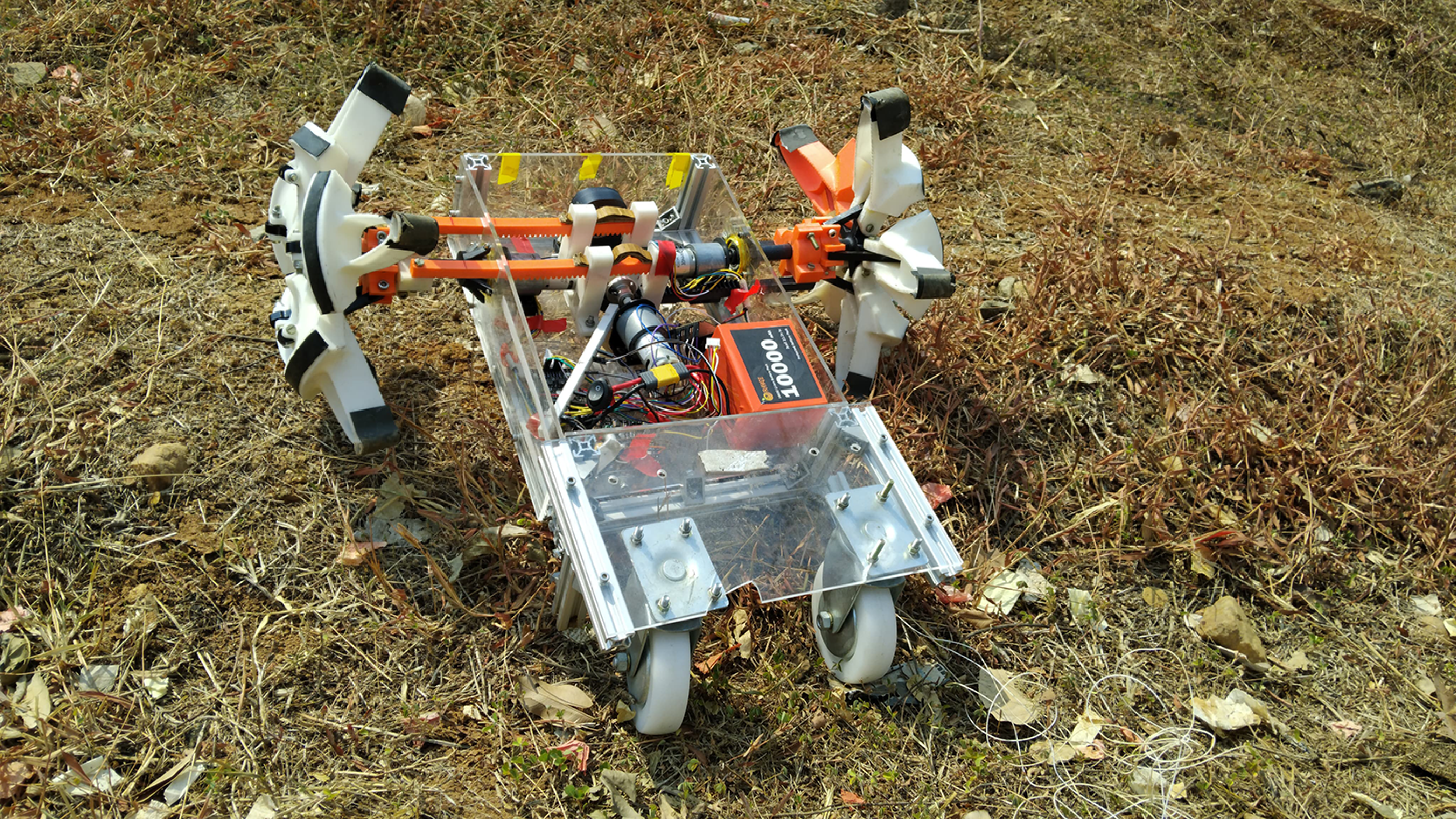
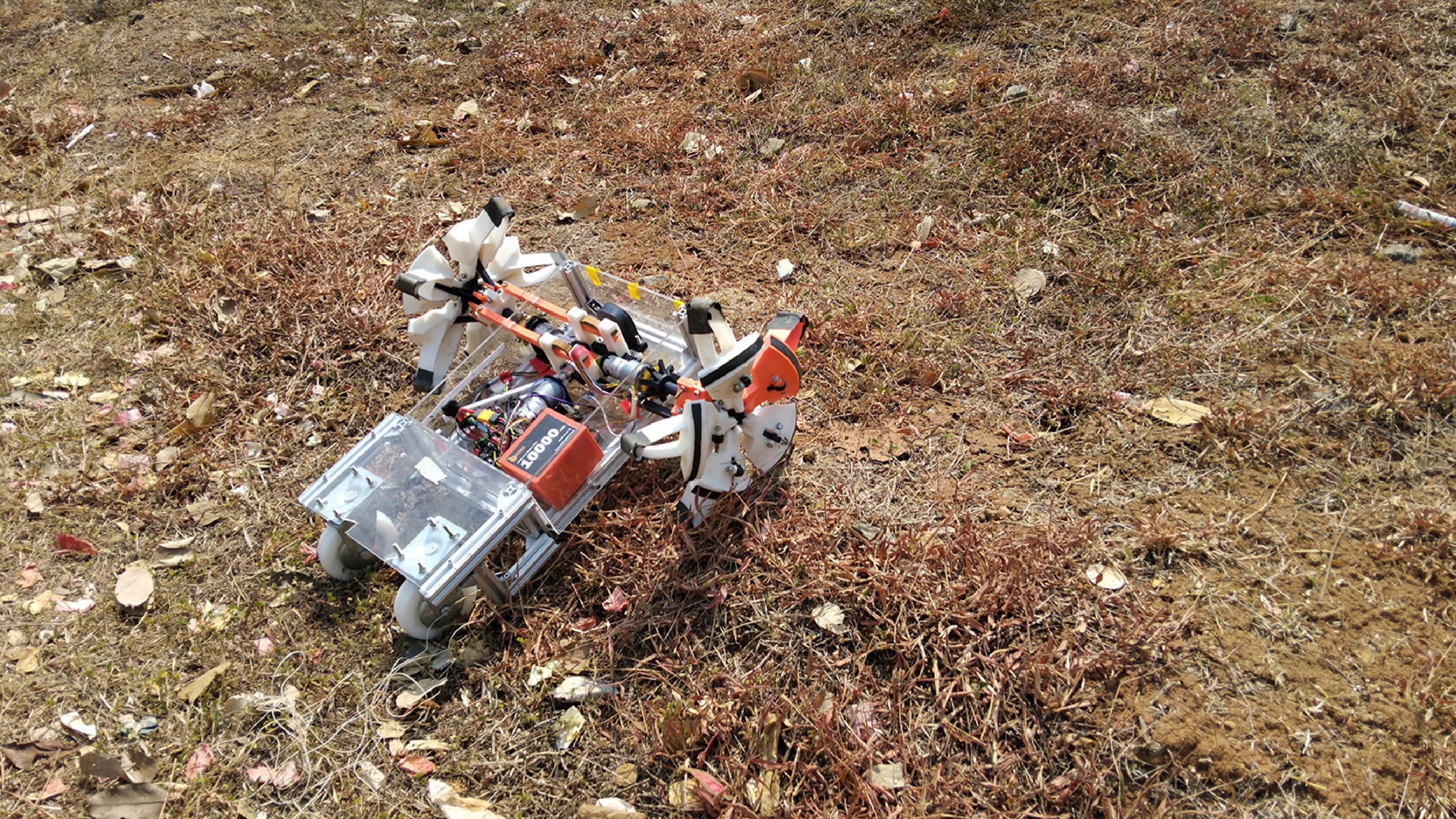
Close-up view of the actual robot.

This paper proposes a method of selection of the actuator required for a mobile robot using three-dimensional dynamic analysis of the whole system. For controlling the robot’s motion to ensure that the robot can follow the desired trajectory, the computed input (Torque) control method is used. Similarly, for driving the robot, two 12-volt, 30 RPM geared DC motors are used, and for the actuation of the wheel reconfiguration mechanism, one 12-volt, 20 RPM DC geared motor is used. Moreover, the CYTRON MDD3A motor driver is used to regulate the current required by the motor. ESP-32 microcontroller is used as the main controller of the robot. The robot platform is powered by a 10,000 mAh Li-ion battery. The subsequent sections of this work are organized as follows. Section 2 describes the method of calculation of wheel and ground normal contact reaction force under longitudinal and lateral dynamics conditions. Section 3 describes the force and torque calculation required by the reconfiguration mechanism used in the wheel of the robot. Section 4 describes the motion of the robot in a three-dimensional environment. Section 5 describes the controller used in the system. Section 6 describes the robot’s hardware integration along with its technical details. Finally, section 7 discusses the simulation results and provides the specification of the actuator required for the reconfiguration.
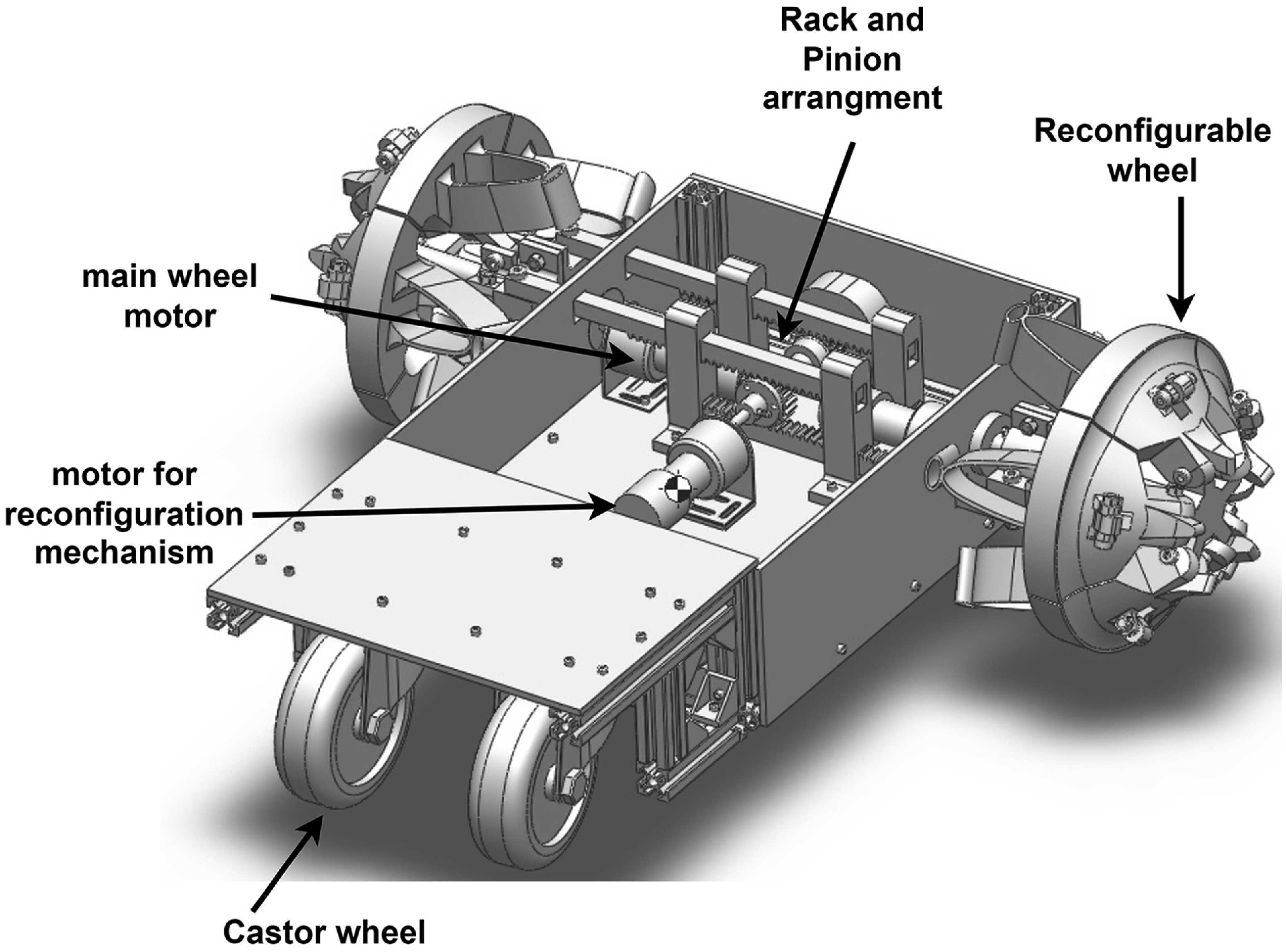
CAD model of the robot.

2. System dynamics
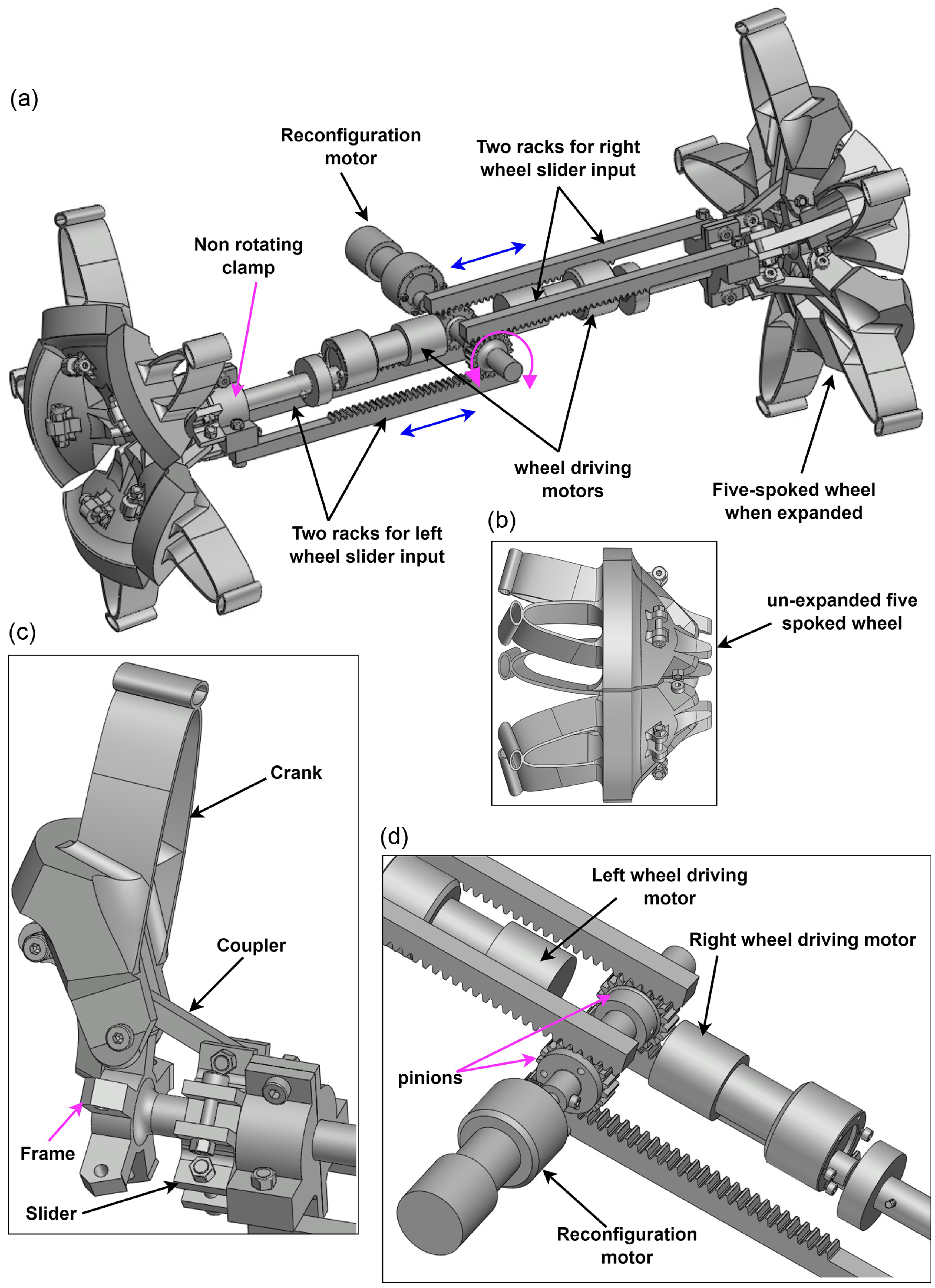
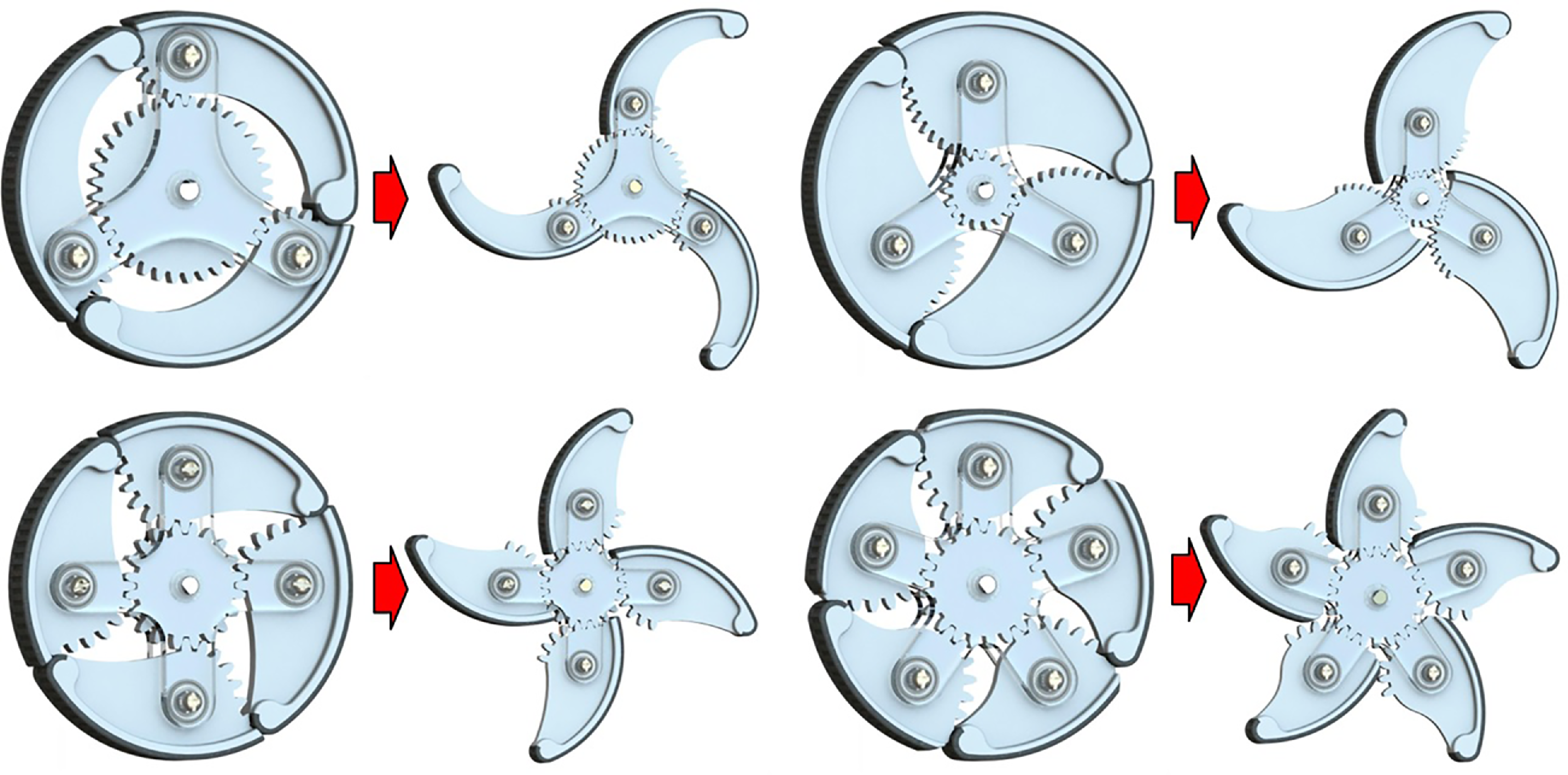
In this work, a slider crank-based reconfiguration mechanism is used in the two front wheels of the robot. Location of these wheels can be seen in the actual picture of the robot as shown in Figure 1 along with the corresponding CAD model in Figure 2. The rear two wheels of the robots are passive caster wheels. The reconfigurable wheel used in this study has two modes of operation. One is wheel mode and another is leg mode. In wheel mode, the front two wheels and rear two caster wheels work together as a four-wheeled mobile robot. However, in legged mode, the front two wheels will turn into a five-spoked wheel and behave as if five legs are rotating around the center of the wheel. The actuation of these legs (wheg mode) is the main role of the reconfiguration mechanism and is shown in Figure 3. There are many variations of reconfiguration mechanisms, through which a normal wheel can be transformed into a spoked one, as discussed in the introduction section. In general, spoke wheel design variations can be broadly classified into out-of-the-wheel-plane reconfiguration and in-the-wheel-plane reconfiguration. In the in-plane-wheel reconfiguration design, spokes of the wheel before reconfiguration and after reconfiguration remain in the same plane, as shown in Figure 4. The advantage of this design is that it is compact, less complex, and requires less number of intermediate links for the transformation, when compared with the out-of-wheel-plane reconfiguration design. However, this design may not be able to sustain the lateral load coming onto the wheel during locomotion in an undulated terrain and may fail due to the absence of any supporting link in this direction. On the contrary, in out-of-wheel-plane reconfiguration design, the transformation of the wheel from a normal wheel to a spoked wheel takes place in a three-dimensional space and requires a larger number of links. Particularly in the present study, five sets of slider crank mechanisms are used in one wheel, which jointly make the one full reconfigurable wheel when assembled, as shown in Figure 3. In each of the wheels, the crank is connected to the corresponding coupler link, the coupler link is connected to the slider, and the slider is connected to the two racks (rack gears). These racks are engaged with the pinion gear, and the pinion gear is directly mounted onto the output shaft of the reconfiguration motor. When the motor rotates the pinion gear, it converts the rotary motion into linear motion of the rack and consequently the slider. For more understanding, an animation of the working mechanism can be seen with this link. Once the sliders on either side of the wheel start moving outward, the wheel expands into the spoked configuration in a three-dimensional space like an umbrella and confirms the legged configuration of the system. Since in this configuration there are multiple links like couplers of each mechanism, which can easily handle the lateral load coming on the wheel due to the terrain undulation, and hence can provide sturdiness to the wheel. Also, to make sure that the wheel can sustain those external loads, particularly lateral loads, the full dynamics of the wheel and its supporting mechanism will be discussed in the reconfiguration dynamics section. This section explores the dynamics of the robot as a four-wheeled vehicle traversing longitudinal and lateral slopes. This study will elucidate the relationship between the contact reaction force of the wheel and the ground under the vehicle’s rolling and pitching circumstances. The normal reaction force will primarily be used to calculate the motor torque necessary for the wheel reconfiguration process, which will be addressed in the reconfiguration dynamics section. Furthermore, in the robot dynamics section, the vehicle’s motion will be simulated along a 3D trajectory, allowing for a comparison of the torque requirements of the actuator under longitudinal and lateral gradient circumstances, so facilitating the finalization of motor selection.
Out of the plane reconfiguration of the spoked wheel. (a) The front two reconfigurable legged-wheels are in legged mode, (b) wheel in compact form. (c) One set of a two-dimensional slider crank mechanism. (d) Close-up view of the rack and pinion arrangement for both front right and front left sides of the wheel with one reconfiguration motor.

Planar reconfiguration of the spoked wheel [Reference Zheng and Lee24].

2.1. Longitudinal dynamics
2.1.1. Robot is in wheel mode
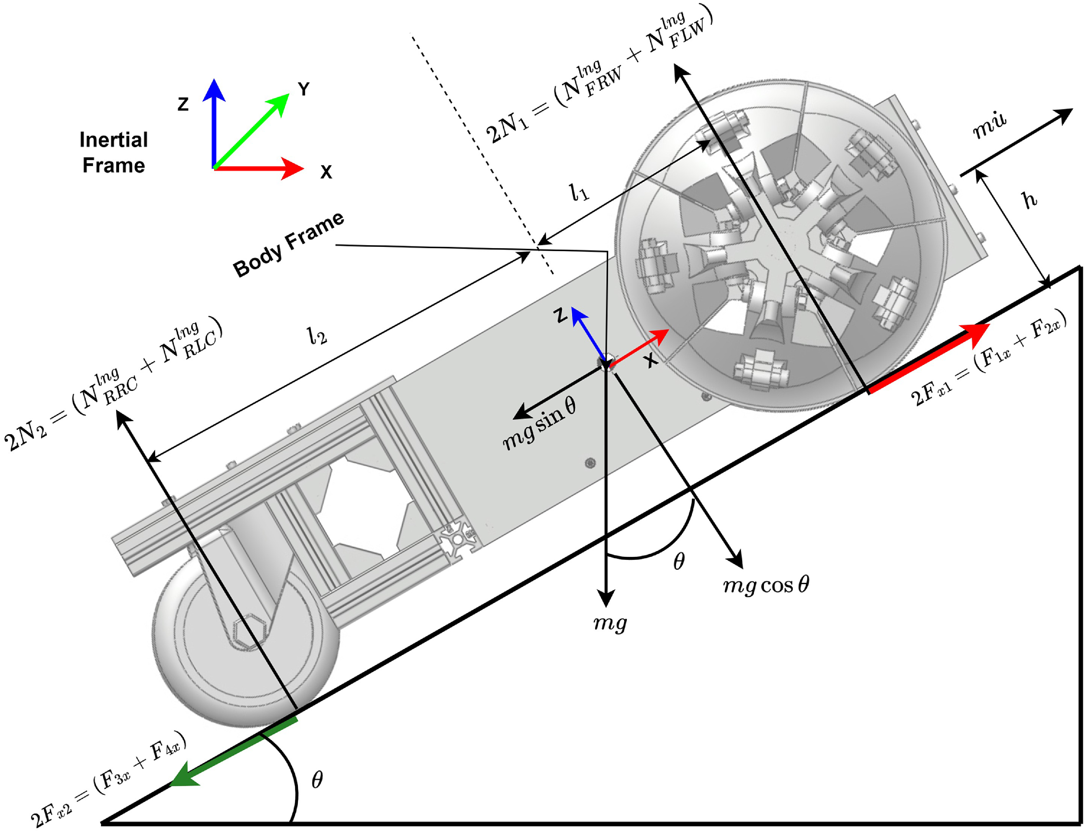
In this case, the front wheels of the robot are not reconfigured, and the robot is considered in the wheel mode. Here, it is assumed that the vehicle or robot is moving on an inclined plane, with a wedge angle of ‘
 $\theta$
’. In addition, this angle can be considered as the vehicle’s pitch motion about the Y-axis of the inertial frame. Here, it is assumed that there is equal normal reaction (i.e.
 ${\mathbf{N_{2}}}$
) on a pair of two caster wheels located on the rear side; similarly, the normal reaction (i.e
 ${\mathbf{N_{1}}}$
) is equal on a pair of front reconfigurable wheels located on the front side of the robot. So, considering the dynamic equilibrium of the system in the x-z plane as shown in Figure 5.
 \begin{equation} \sum F_{x}=m\dot {u} \,:\, 2F_{x1}-2F_{x2}-mgsin\theta = m\dot {u} \end{equation}
where
 $F_{x1}$
is the traction force in the positive
 $X$
direction on the front powered wheels.
 $F_{x2}$
is the friction force on the rear caster wheels and will be in the negative
 $X$
direction.
 $m$
is the total mass of the system, and
 $\dot {u}$
is the linear acceleration component of the robot in the X direction with respect to the body frame of the robot. Force,
 $F_{x1}=F_{1x}=F_{2x}=\mu _{x}{\mathbf{N_{1}}}$
, where
 $\mu _{x}$
is the coefficient of friction between the wheel and surface contact point along the
 $X$
axis of the vehicle frame. Since in our system, only the front two wheels are powered by motors, the rear caster wheels receive the traction or driving force indirectly from the front two wheels, so for the rear caster wheels, we have
 $F_{x2} = F_{3x}=F_{4x}\leq \mu _{x}{\mathbf{N_{2}}}$
, which ensures no slip condition or perfect rolling condition. Therefore, we can write
 \begin{equation} \sum F_{z}=0 \,:\, 2{\mathbf{N_{1}}}+2{\mathbf{N_{2}}}-mgcos\theta =0 \end{equation}
 \begin{equation} \sum M_y^{COM}=0 \,:\, 2{\mathbf{N_{1}}}l_{1}-2{\mathbf{N_{2}}}l_{2}+2F_{x1}h-2F_{x2}h=0 \end{equation}
Longitudinal dynamics in wheel mode.

 $M_{y}^{COM}$
denotes the moment at the center of mass (COM) about
 $Y$
-axis of the vehicle frame.
 $l_{1}$
and
 $l_{2}$
denote the distances from the COM to the center of the front wheel and the center of the rear caster, respectively, along the
 $X$
-axis of the vehicle frame. Likewise,
 $h$
denotes the height of the COM above the ground. Eqs. (1), (2) and (3) are reduced into two independent equations in two variables
 ${\mathbf{N_{1}}}$
and
 ${\mathbf{N_{2}}}$
, which can be represented in matrix form as:
 \begin{equation} \begin{bmatrix} 2 & 2\\[2pt]2l_{1} & -2l_{2} \end{bmatrix}\begin{bmatrix} {\mathbf{N_{1}}}\\[2pt]{\mathbf{N_{2}}} \end{bmatrix}=\begin{bmatrix} mg\cos {\theta }\\[2pt]-mgh\sin {\theta }-m\dot {u}h \end{bmatrix} \end{equation}
which on solving gives
 \begin{equation} {\mathbf {N}_{1}}={\mathbf {N}}_{FRW}^{lng}={\mathbf {N}}_{FLW}^{lng}=\frac {mgl_{2}\cos {\theta }}{2l}-\frac {m\dot {u}h+mgh\sin {\theta }}{2l} \end{equation}
and
 \begin{equation} {\mathbf {N}}_{2}={\mathbf {N}}_{RRC}^{lng}={\mathbf {N}}_{RLC}^{lng}=\frac {m\dot {u}h+mgh\sin {\theta }}{2l}+\frac {mgl_{1}\cos {\theta }}{2l} \end{equation}
 ${\mathbf {N}}_{FRW}^{lng}$
denotes the normal reaction on the front right wheel in longitudinal dynamics,
 ${\mathbf {N}}_{FLW}^{lng}$
signifies the normal reaction on the front left wheel in longitudinal dynamics,
 ${\mathbf {N}}_{RRC}^{lng}$
represents the normal reaction on the rear right caster in longitudinal dynamics, and
 ${\mathbf {N}}_{RLC}^{lng}$
indicates the normal reaction on the rear left caster in longitudinal dynamics. Furthermore,
 $ l_{1} + l_{2} = l$
, representing the entire length from the center of the front wheels to the center of the rear casters along the longitudinal direction of the vehicle. Moreover, here it is important to note that the normal reactions on the front two pair wheels are assumed to be equal, and so is with the rear two castors. Since in the present analysis, gradient of the terrain is considered only about the Y-axis of the inertial frame; however, if the gradient is present in both about X- and Y-axes of the inertial frame, in case of a highly unstructured terrain, then the normal reactions obtained in longitudinal dynamics and lateral dynamics (discussed in lateral dynamics subsection) must be compared and whichever appears higher in magnitude, should be considered as final.
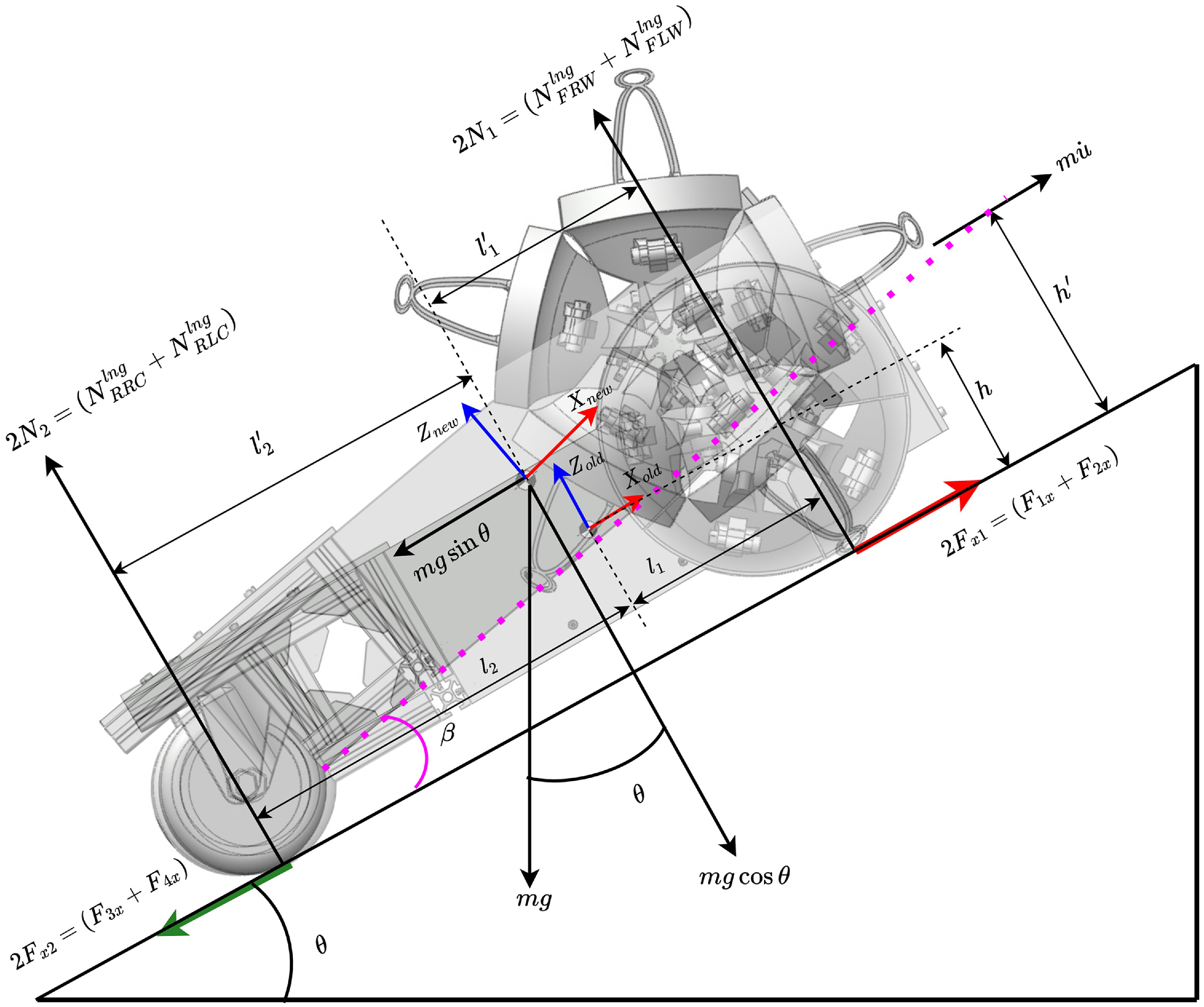
Longitudinal dynamics in legged mode.

2.1.2. Robot is in leg mode
The front two wheels of the robot are regarded in the legged mode upon reconfiguration, as seen in Figure 6. Due to the reconfiguration of the wheel, altering the position of the COM and therefore the normal reaction forces on the wheels, the normal reaction on the front and rear wheels will be recalculated, based on the new COM location for the leg mode. The COM shift arises from the unfolding of the front two wheels, resulting in the robot body rotating around the contact point of the rear caster wheels and the ground by an angle of
 $\beta =10.25^\circ$
, in an anti-clockwise direction around the vehicle frame’s
 $Y$
-axis. Consequently, to get the new coordinates of the COM, we may multiply the previous coordinates of the COM by the rotation matrix corresponding to the angle (
 $-\beta$
) around the
 $Y$
-axis of the vehicle frame. So, we now possess two frames, old and new, corresponding to the robot’s previous and current COM. The updated coordinates of the new COM, relative to the world frame, may be computed as follows:
 \begin{equation} \begin{bmatrix} X_{new}\\[2pt]Y_{new}\\[2pt]Z_{new} \end{bmatrix}=\begin{bmatrix} \cos {(-\beta )} &\quad 0 &\quad \sin {(-\beta )}\\[2pt] 0 &\quad 1 &\quad 0\\[2pt] -\sin {(-\beta )} &\quad 0 &\quad \cos {(-\beta )} \end{bmatrix}\begin{bmatrix} l_{2}\\[2pt]0\\[2pt]h \end{bmatrix} \end{equation}
through which we can obtain the expression for
 $l_{2}^{\prime}$
,
 $l_{1}^{\prime}$
, and
 $h^{\prime}$
as follows:
 \begin{equation} l^{\prime}_{2}=l_{2}cos\beta -hsin\beta \end{equation}
 \begin{equation} h^{\prime}=l_{2}sin\beta +hcos\beta \end{equation}
where
 $l_{1}^{\prime}=l-l^{\prime}_{2}$
, since
 $l_{1}+l_{2}=l=l_{1}^{\prime}+l^{\prime}_{2}$
. Now substituting the expression of
 $l_{1}^{\prime}$
,
 $l^{\prime}_{2}$
, and
 $h^{\prime}$
in place of
 $l_{1}$
,
 $l_{2}$
, and
 $h$
, respectively, from Eqs. (8) and (9) into Eqs. (5) and (6). Which gives us new expressions for the normal reactions in leg mode, as given below
 \begin{equation} {\mathbf {N}}_{1}={\mathbf {N}}_{FRW}^{lng}={\mathbf {N}}_{FLW}^{lng}=\frac {mgl_{2}^{\prime}\cos {\theta }}{2l}-\frac {m\dot {u}h^{\prime}+mgh^{\prime}\sin {\theta }}{2l} \end{equation}
 \begin{equation} {\mathbf {N}}_{2}={\mathbf {N}}_{RRC}^{lng}={\mathbf {N}}_{RLC}^{lng}=\frac {m\dot {u}h^{\prime}+mgh^{\prime}\sin {\theta }}{2l}+\frac {mgl_{1}^{\prime}\cos {\theta }}{2l} \end{equation}
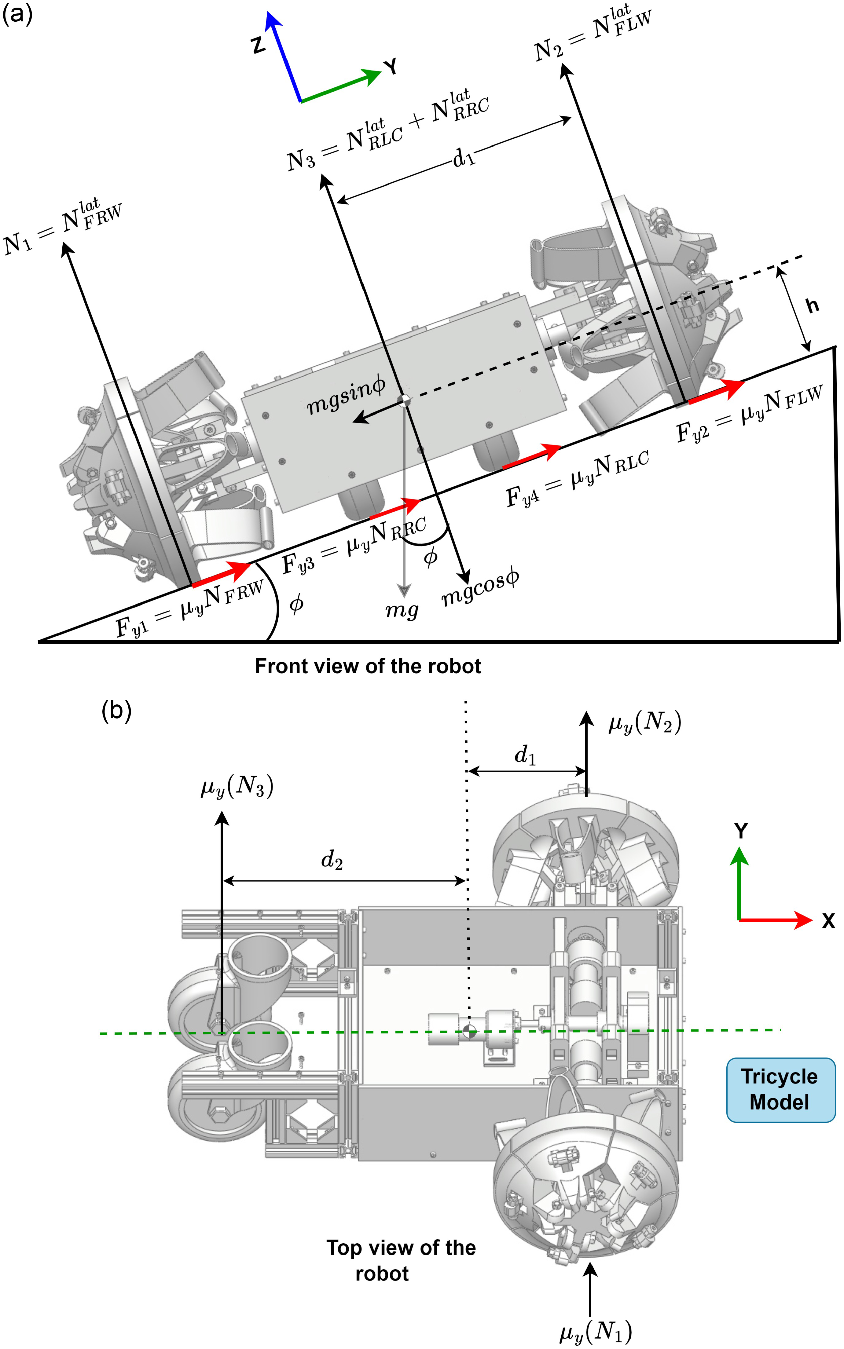
Robot is in wheel mode and resting on the banked surface.

2.2. Lateral dynamics
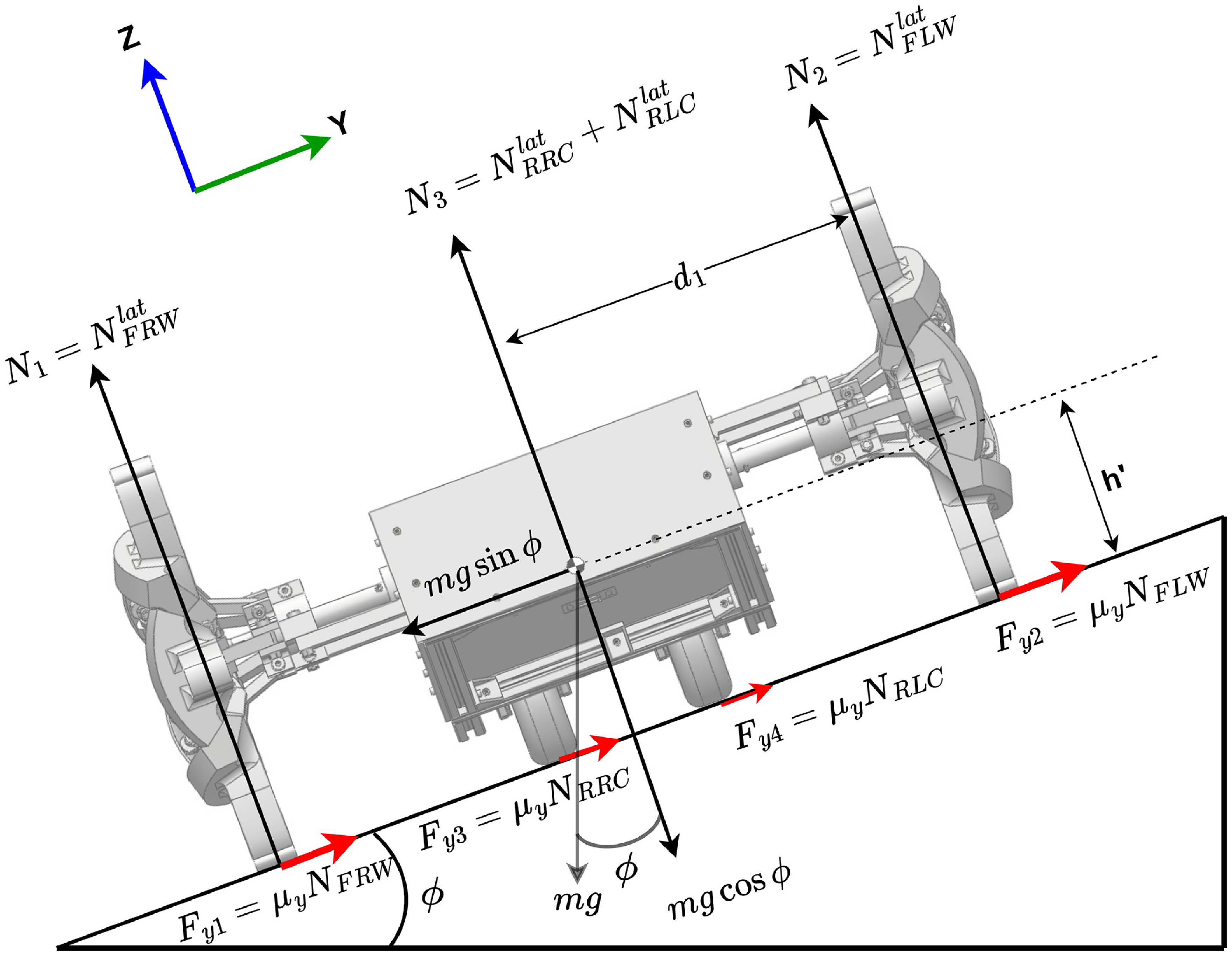
This section aims to elucidate the robot’s rolling dynamics. In this case, since the robot is inclined on a banked surface laterally which the normal reaction on the right side wheel and left side wheel will be different. Additionally, robot’s front wheels and rear wheels, which are casters in the present case, are not inline like an ordinary passenger vehicle, therefore reaction on the left side (both front and rear) wheels cannot be considered equal to the right side (both front and rear) wheels, and hence all four wheels will have different normal reactions. Moreover, in the lateral dynamics case, the robot can be considered in the Y-Z plane, and only three independent equations can be obtained through equilibrium equations corresponding to four unknowns, and hence closed-loop analytical solution for all four normal reactions is not possible. Therefore, it is decided to consider the present case of lateral dynamics by assuming the four wheel robot model as a three wheel tricycle model, since rear two passive caster wheels of the robot are very close to the centerline (6 cm away) or the longitudinal axis, compared to front two wheels, which are 21.6 cm away from the longitudinal axis. So in the lateral dynamics study, the rear two casters are considered as one caster located along the centerline or the longitudinal axis of the system. Additionally, we need three independent equations to find three normal reactions, for which the robot’s top view is also considered to get the third independent equation required for the solution. Now, the height of the COM from the ground in wheel mode is denoted as
 $h$
, whereas in legged mode it is represented as
 $h'$
, as seen in Figs. 7 and 8, respectively. Moreover, as previously shown in the longitudinal dynamics, the reconfiguration of the robot’s wheel will result in changes only to
 $l_{1}$
,
 $l_{2}$
, and
 $h$
, while the remaining expressions will stay unchanged. Therefore, in this section, we will derive the mathematical expressions for the normal reaction in legged mode directly, and by substituting the angle
 $\beta$
with
 $\beta =0$
, the result will correspond to the wheel mode. So, now considering the equilibrium conditions:
 \begin{equation} \sum {F_{y}}= 0 \,:\, \mu _{y}({\mathbf{N_{1}}}+{\mathbf{N_{2}}}+\mathbf{N_{3}})-mg\sin {\phi }= 0 \end{equation}
 \begin{equation} \sum F_{z}= 0 \,:\, {\mathbf{N_{1}}}+{\mathbf{N_{2}}}+{\mathbf{N_{3}}}-mg\cos {\phi }= 0 \end{equation}
 \begin{equation} \sum M_{x}^{COM}= 0 \,:\, -{\mathbf{N_{1}}}d_{1}+{\mathbf{N_{2}}}d_{1}+mgh^{\prime}\cos {\phi }= 0 \end{equation}
Robot is in the leg mode and resting on the banked surface.

Eqs. (12), (13), and (14) are two independent equations in three variables
 ${{\mathbf {N}}_{1}}$
(normal reaction on the front right wheel),
 ${\mathbf {N}}_{2}$
(normal reaction on the front left wheel) and
 ${\mathbf {N}}_{3}$
(normal reaction on the two rear casters). So one more independent equation is required to solve for three variables, and this equation can be found from the sub-figure (b) of the Figure 7, by taking the moment about the Z axis of the vehicle frame at the COM, as given below:
 \begin{equation} \sum M_{z}^{COM}=0 \,:\, \mu _{y}({\mathbf{N_{1}}}+{\mathbf{N_{2}}})l_{1}-\mu _{y}\mathbf{N_{3}}l_{2}=0 \end{equation}
Now, arranging the three independent equations in the matrix form as:
 \begin{equation} \begin{bmatrix} 1 &\quad 1 &\quad 1\\[2pt]-d_{1} &\quad d_{1} &\quad 0\\[2pt] \mu _{y}l_{1} &\quad \mu _{y}l_{1} &\quad -\mu _{y}l_{2} \end{bmatrix}\begin{bmatrix} {\mathbf{N_{1}}}\\[2pt]{\mathbf{N_{2}}}\\[2pt] {\mathbf{N_{3}}} \end{bmatrix}=\begin{bmatrix} mg\cos {\phi }\\[2pt]-mgh'\sin {\phi }\\[2pt] 0 \end{bmatrix} \end{equation}
On solving Eq. (16), normal reactions on all three wheels can be represented as given below:
 \begin{equation} {{\mathbf {N}}_{1}}={\mathbf {N}}_{FRW}^{lat}= \frac {mgd_{1}l_{2}\cos {\phi }+h^{\prime}l_{1}\sin {\phi }+h^{\prime}l_{2}\sin {\phi }}{2d_{1}(l_{1}+l_{2})} \end{equation}
 \begin{equation} {\mathbf {N}}_{2}={\mathbf {N}}_{FLW}^{lat} = \frac {-mgh^{\prime}l_{1}\sin {\phi }+d_{1}l_{2}\cos {\phi }+h^{\prime}l_{2}\sin {\phi }}{2d_{1}(l_{1}+l_{2})} \end{equation}
 \begin{equation} {\mathbf {N}}_{RRC}^{lat} = {\mathbf {N}}_{RLC}^{lat}=\frac {{\mathbf {N}}_{3}}{2}=\frac {mgl_{1}\cos {\phi }}{2(l_{1}+l_{2})} \end{equation}
where
 ${\mathbf {N}}_{FRW}^{lat}$
,
 ${\mathbf {N}}_{FLW}^{lat}$
,
 ${\mathbf {N}}_{RRC}^{lat}$
, and
 ${\mathbf {N}}_{RLC}^{lat}$
are the normal reaction on the front right wheel, front left wheel, rear right caster, and rear left caster in the lateral dynamics, respectively. Additionally,
 $\mu _{y}$
is the coefficient of static friction between the wheel and ground along the Y-axis of the vehicle frame. Normal reaction calculated in lateral and longitudinal dynamics, as derived above, will be useful to assess the stability of the robot in motion and to calculate the amount of input force required in the reconfiguration mechanism, used in both front wheels of the robot, which is discussed in the next section.
Reconfiguration mechanism in assembled and free state.

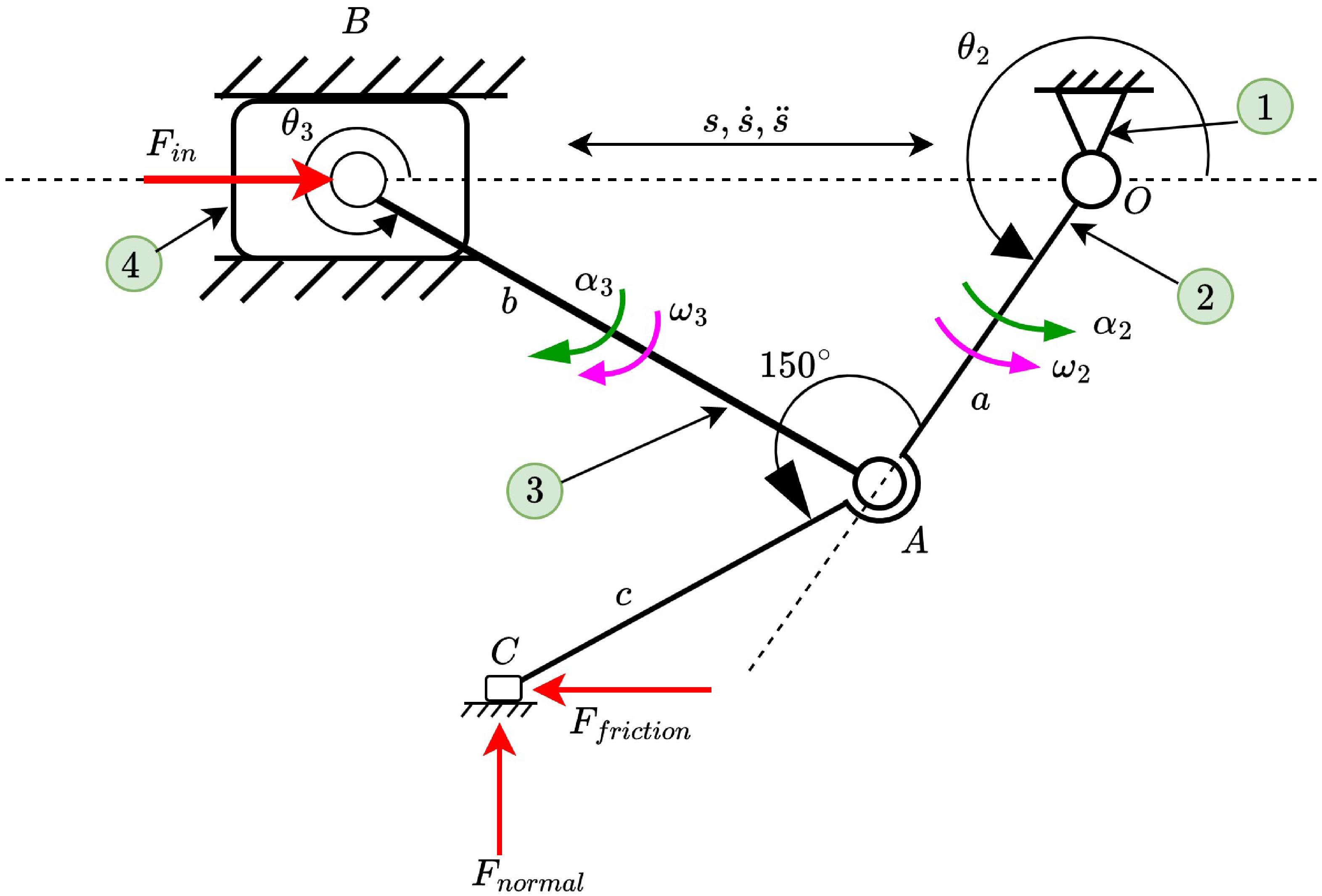
Kinematic diagram of slider crank mechanism.

3. Reconfiguration dynamics
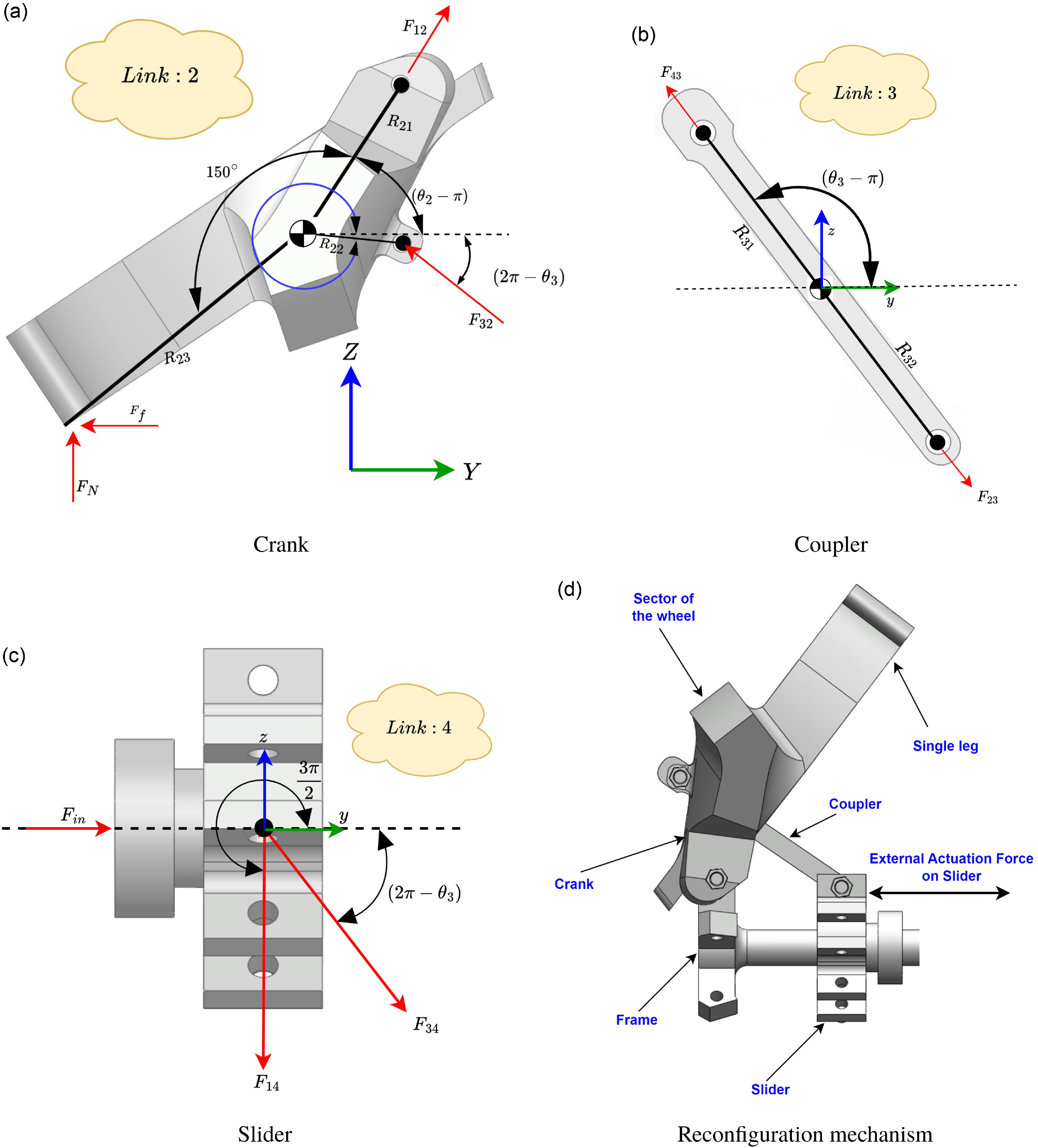
This section elucidates the dynamics of the mechanism used for wheel reconfiguration. This study employs the slider crank mechanism for reconfiguration, as seen in Figure (9d). Five such identical mechanisms are used in each wheel to provide smooth opening and closing of the same. Each mechanism is activated by the external force applied to the slider, facilitated by a motor and a rack and pinion mechanism housed inside the main body. The output shaft of the reconfiguration motor is connected to two pinion gears, which are connected to the same shaft since a single motor operates both side wheels. The slider obtains the input force from the reconfigurable motor through the rack and pinion mechanism connecting the slider and the motor. The coupler link converts the slider’s linear motion into the crank’s angular motion, as seen in Figure 10. The crank’s design integrates the characteristics of the wheel and the legs, relying only on the crank’s angular position. The angular position of the crank is dependent upon the slider. Consequently, this dynamic study aims to determine the input force necessary for the actuation of the reconfiguration mechanism, considering the normal reaction on the wheel and the frictional force between the wheel and the ground. During the reconfiguration process, the frictional force acting between the wheel and the ground will counteract the motion generated by the mechanism. Consequently, it is essential to determine the input force necessary at the slider for the effective implementation of the reconfiguration mechanism. Upon calculating this force, it will facilitate the selection of the appropriate motor for the reconfiguration procedure. In the dynamic analysis, each link is analyzed individually to determine the forces acting on the respective joints. From Figure (9a), we may formulate the equilibrium equations for the crank as follows:
 \begin{equation} F_{12y}-F_{32y}=m_{2}a_{2y}+\mu _{y}{\mathbf{F_{N}}} \end{equation}
 \begin{equation} F_{12z}+F_{32z}=m_{2}a_{2z}-{\mathbf{F_{N}}} \end{equation}
 \begin{equation} R_{21y}F_{12z}-R_{21z}F_{12y}+R_{22y}F_{32z}-R_{22z}F_{32y}=\mu R_{23z}{\mathbf{F_{N}}}-R_{23y}F_{N}+I_{2}\boldsymbol{\alpha _{2}} \end{equation}
where
 ${\mathbf{F_{12}}}$
is the force on link 2 due to link 1,
 ${\mathbf{F_{32}}}$
is the force on link 2 due to link 3,
 $I_{2}$
is the moment of inertial of link 2,
 ${\mathbf{a_{2}}}$
and
 $\boldsymbol{\alpha _{2}}$
are the linear and angular acceleration of the link 2, and
 ${\mathbf{F_{N}}}$
is the normal contact reaction force at the wheel. Now, corresponding to the Figure (9b), for coupler, we can write as:
 \begin{equation} F_{23y}-F_{43y}=m_{3}a_{3y} \end{equation}
 \begin{equation} F_{43z}-F_{23z}=m_{3}a_{3z} \end{equation}
 \begin{equation} R_{31y}F_{43z}-R_{31z}F_{43y}-R_{32y}F_{32z}+R_{32z}F_{32y}=I_{3}\boldsymbol{\alpha _{3}} \end{equation}
where
 ${\mathbf{F_{43}}}$
is the force on link 3 due to link 4,
 ${\mathbf{F_{23}}}$
is the force on link 3 due to link 2,
 $I_{3}$
is the moment of inertia of link 3, and
 ${\mathbf{a_{3}}}$
and
 $\boldsymbol{\alpha _{3}}$
are the linear and angular acceleration of link 3. Likewise, corresponding to Figure 9c, for slider, we can write as:
 \begin{equation} {\mathbf{F_{in}}}-\mu _{y}sign(\boldsymbol{\dot {s}})|F_{14z}|+F_{34y}=m_{4}a_{4y} \end{equation}
 \begin{equation} F_{34z}+F_{14z}=0 \end{equation}
where
 ${\mathbf{F_{in}}}$
is the input force to the slider,
 ${\mathbf{F_{14}}}$
is the force on link 4 due to link 1,
 ${\mathbf{F_{34}}}$
is the force on link 4 due to link 3,
 $\boldsymbol{\dot {s}}$
is the slider velocity, and
 ${\mathbf{a_{4}}}$
is the slider acceleration. In the case of a slider, due to its exclusively linear motion, its angular acceleration is therefore zero, i.e.,
 $\boldsymbol{\alpha _{4}}$
= 0. Furthermore, owing to its constrained motion along the y-axis, there will be no acceleration in the z-direction; hence,
 $a_{4z}=0$
. All the aforementioned dynamic equations for the mechanism are articulated within the same reference frame as the vehicle frame, meaning that the individual axes of the vehicle frame align with the respective local coordinate frames of the links. Consequently, no additional transformation is necessary, allowing for the direct resolution of these equations. Now, since Eqs. (20) through (27) are required to be solved simultaneously. Therefore, these equations are arranged in the matrix form as shown below:
 \begin{equation} \begin{bmatrix} 1 & 0 & -1 & 0 & 0 & 0 & 0 & 0\\[3pt] 0 & 1 & 0 & 1 & 0 & 0 & 0 & 0\\[3pt] -R_{21z} & R_{21y} & -R_{22z} & R_{22y} & 0 & 0 & 0 & 0\\[3pt] 0 & 0 & -1 & 0 & -1 & 0 & 0 & 0\\[3pt] 0 & 0 & 0 & 1 & 0 & 1 & 0 & 0\\[3pt] 0 & 0 & R_{32z} & -R_{32y} & -R_{31z} & R_{31y} & 0 & 0\\[3pt] 0 & 0 & 0 & 0 & -1 & 0 & -\mu _{y} sign(\dot {\mathbf {s}}) & 1\\[3pt] 0 & 0 & 0 & 0 & 0 & 1 & -1 & 0 \end{bmatrix}\begin{bmatrix} F_{12y}\\[3pt]F_{12z}\\[3pt]F_{32y}\\[3pt]F_{32z}\\[3pt]F_{43y}\\[3pt]F_{43z}\\[3pt]F_{14z}\\[3pt] {\mathbf{F_{in}}} \end{bmatrix}=\begin{bmatrix} m_{2}a_{2y}+\mu _{y} {\mathbf{F_{N}}}\\[3pt]m_{2}a_{2z}-{\mathbf{F_{N}}}\\[3pt]R_{23z}\mu _{y} {\mathbf{F_{N}}}-R_{23y}{\mathbf{F_{N}}}+I_{2}\boldsymbol{\alpha _{2}}\\[3pt]m_{3}a_{3y}\\[3pt] m_{3}a_{3z}\\[3pt]I_{3}\boldsymbol{\alpha _{3}}\\[3pt]m_{4}a_{4y}\\[3pt]0 \end{bmatrix} \end{equation}
Upon resolving Eq. (28), we may ascertain all the joint forces inside the mechanism, including the
 ${\mathbf{F_{in}}}$
, which represents the input force necessary at the slider. Additional joint forces derived from this equation can be used to design the individual link by specifying the necessary cross-sectional area, suitable material, and safety factor. The expression for
 ${\mathbf{F_{in}}}$
is shown below:
 \begin{eqnarray} {\mathbf{F_{in}}} &=& \frac {\mathbf{F_{N}}(\sigma _{1}-\mu _{y}\sigma _{2})+I_{3}\boldsymbol{\alpha _{3}}\sigma _{3}+m_{2}\sigma _{4}+m_{3}\sigma _{5}+m_{4}\sigma _{6}+sign(\dot {\mathbf {s}})\mu _{y}\sigma _{7}}{2} \nonumber\\[8pt] && +\frac {\mathbf{F_{N}}\mu _{y}sign(\dot {\mathbf {s}})\sigma _{8}+\mu _{y}sign({\dot {\mathbf {s}}})\sigma _{9}+{\mathbf{F_{N}}}\mu _{y}^{2}sign(\dot {\mathbf {s}})\sigma _{10}}{2} \end{eqnarray}
where
 \begin{equation} \sigma _{1}=R_{32y}^2-R_{21y}R_{31y}-R_{21y}R_{32y}+R_{31y}R_{32y} \end{equation}
 \begin{equation} \sigma _{2}=R_{21z}R_{31y}+R{21z}R_{32y}-R_{31y}R_{32z}-R_{32y}R_{32z} \end{equation}
 \begin{equation} \sigma _{3}=R_{21y}-R_{22y}-R_{31y}-R_{32y} \end{equation}
 \begin{equation} \sigma _{4}=-R_{21z}R_{31y}a_{2y}+R_{21y}R_{31y}a_{2z}+R_{21y}R_{32y}a_{2z}-R_{21z}R_{32y}a_{2y} \end{equation}
 \begin{eqnarray} \sigma _{5} &=& -R_{21y}R_{31y}a_{2y}+R_{21z}R_{31y}a_{3y}+R_{21y}R_{32z}a_{3y}+R_{21z}R_{32y}a_{3y}+R_{22y}R_{31y}a_{3z} \nonumber\\[8pt] && +R_{22z}R_{31y}a_{3y}+R_{22y}R_{32z}a_{3y}+R_{22z}R_{32y}a_{3y} \end{eqnarray}
 \begin{eqnarray} \sigma _{6} &=& -R_{21y}R_{31z}a_{4y}-R_{21z}R_{31y}a_{4y}-R_{21y}R_{32z}a_{4y}-R_{21z}R_{32y}a_{4y} \nonumber\\[8pt] && +R_{22y}R_{31z}a_{4y}-R_{22z}R_{31y}a_{4y}+R_{22y}R_{32z}a_{4y}-R_{22z}R_{32y}a_{4y} \end{eqnarray}
 \begin{eqnarray} \sigma _{7} &=& -R_{21y}R_{31z}a_{2z}+R_{21z}R_{31z}a_{2y}-R_{21y}R_{32z}a_{2z}m_{2}+R_{21z}R_{32z}a_{2y}m_{2}+R_{21y}R_{31z}a_{3z}m_{3} \notag \\[8pt] && -R_{21z}R_{31z}a_{3y}m_{3}+R_{21y}R_{32z}a_{3z}m_{3}+R_{21z}R_{32y}a_{3y}m_{3}\\[8pt] \notag && -R_{22y}R_{31z}a_{3z}m_{3}-R_{22z}R_{31z}a_{3y}m_{3}-R_{22y}R_{32z}a_{3z}m_{3}+R_{22z}R_{32y}a_{3z}m_{3} \end{eqnarray}
 \begin{equation} \sigma _{8}=R_{21y}R_{31z}+R_{21y}R_{32z}-R_{31z}R_{32y}-R_{32y}R_{32z} \end{equation}
 \begin{equation} \sigma _{9}=I_{3}\boldsymbol{\alpha _{3}}(R_{21z}R_{22z})+I_{2}\boldsymbol{\alpha _{2}}(R_{31z}+R_{32z}) \end{equation}
 \begin{equation} \sigma _{10}=R_{21z}R_{31z}+R_{21z}R_{32z}+R_{31z}R_{32z} \end{equation}
Since the expression for the input force (
 ${\mathbf{F_{in}}}$
) contains the linear and angular acceleration terms, which have already been determined from the study of position, velocity, and acceleration analysis. These accelerations and angular velocities are also provided below:
 \begin{equation} \boldsymbol{\alpha _{2}}=\frac {a\cos ({\theta _{3}-\theta _{2}})\boldsymbol{\omega _{2}}^{2}-b\boldsymbol{\omega _{3}}^{2}-\ddot {\mathbf {s}}\cos {\theta _{3}}}{a\sin ({\theta _{3}-\theta _{2}})} \end{equation}
 \begin{equation} \boldsymbol{\alpha _{3}}=\frac {-a\boldsymbol{\omega _{2}}^{2}+b\cos ({\theta _{2}-\theta _{3}})\boldsymbol{\omega _{3}}^{2}-\ddot {\mathbf {s}}\cos {\theta _{2}}}{b\sin ({\theta _{2}-\theta _{3}})} \end{equation}
 \begin{equation} a_{2y}=-R_{21}\boldsymbol{\omega _{2}}^{2}\cos {\theta _{2}}-R_{21}\boldsymbol{\alpha _{2}}\sin {\theta _{3}} \end{equation}
 \begin{equation} a_{2z}=-R_{21}\boldsymbol{\omega _{2}}^{2}\sin {\theta _{2}}+R_{21}\boldsymbol{\alpha _{2}}\cos {\theta _{2}} \end{equation}
 \begin{equation} a_{3y}=-a\boldsymbol{\omega _{2}}^{2}\cos {\theta _{2}}-a\boldsymbol{\alpha _{2}}\sin {\theta _{2}}-R_{32}\boldsymbol{\omega _{3}}^{2}\cos {\theta _{3}}-R_{32}\boldsymbol{\alpha _{3}}\sin {\theta _{3}} \end{equation}
 \begin{equation} a_{3z}=-a\boldsymbol{\omega _{2}}^{2}\sin {\theta _{2}}+a\boldsymbol{\alpha _{2}}\cos {\theta _{2}}-R_{32}\boldsymbol{\omega _{3}}^2\sin {\theta _{3}}+R_{32}\boldsymbol{\alpha _{3}}\cos {\theta _{3}} \end{equation}
Similarly, acceleration terms depend on the angular velocities of the links. Therefore, expressions for the angular velocities are given below:
 \begin{equation} \boldsymbol{\omega _{2}}=\frac {b\cos {\theta _{3}}\dot {\mathbf {s}}}{a\cos {\theta _{2}(b\tan {\theta _{2}}\cos {\theta _{3}}}- b\sin {\theta _{3}})} \end{equation}
 \begin{equation} \boldsymbol{\omega _{3}}=\frac {\dot {\mathbf {s}}}{b\tan {\theta _{2}}\cos {\theta _{3}} - b\sin {\theta _{3}}} \end{equation}
In this section, the objective of calculating the input force (
 $F_{in}$
) is to find out the torque required at the reconfiguration motor end, which provides the required input force for executing reconfiguration. Therefore, as we have the expression for the force required at the slider end of the mechanism, we can now calculate the minimum torque required at the motor, as shown below:
 \begin{equation} \boldsymbol{\tau _{m}}=2(r_{p}{\mathbf{F_{in}}}) \end{equation}
where
 $\boldsymbol{\tau _{m}}$
is the torque required by the reconfiguration motor, and
 $r_{p}$
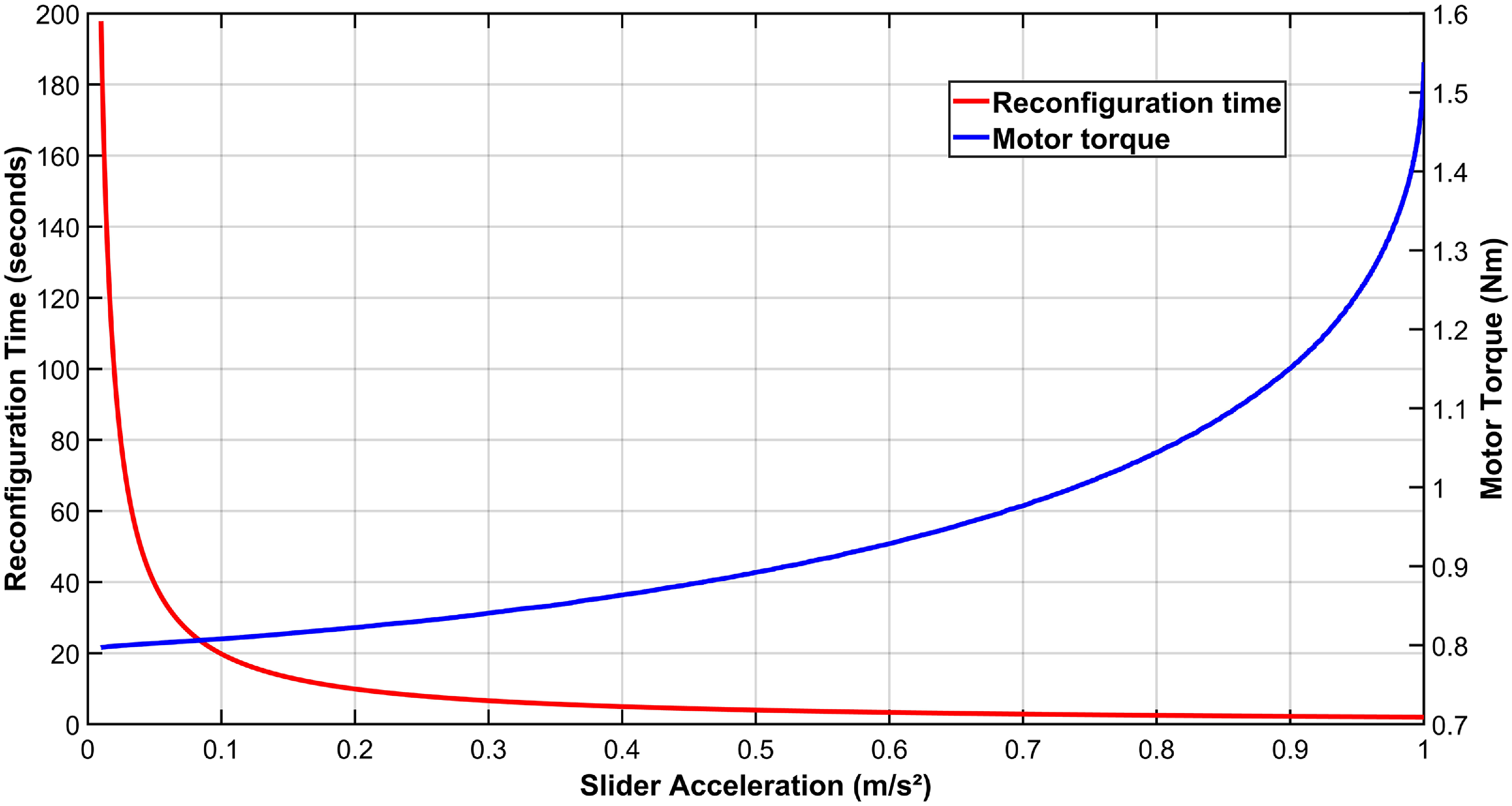
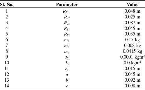
is the radius of the pinion gear (pitch circle radius of the gear) attached to the reconfiguration motor. Since we have two reconfigurable wheels on either side of the motor, and only one motor is used for this purpose, therefore, two times. Now, as the input force required at the slider in Eq. (29) is a function of slider acceleration and the normal reaction at the wheel, which indicates that, if normal reaction onto the wheel increases, so is the motor torque, or vice versa. Furthermore, increasing the slider acceleration can result in reduced reconfiguration time while simultaneously elevating motor torque. This we can verify from the Figure 11. From the figure, we can observe that as the slider acceleration is increased from 0.01 m/s2 to 1 m/s2, reconfiguration time is decreased from 197.78 s to 2 s. Similarly, motor torque corresponding to the 0.01 m/s2 is 0.79 Nm, and corresponding to 1 m/s2, it is 1.58 Nm. For this analysis, a normal reaction of 15 Newtons on each of the front two wheels is considered, and other physical parameters of the reconfiguration mechanism used for this verification are provided in Table VI.
Graphical representation of the actuator selection criterion based on slider acceleration and transformation time.

4. Robot dynamics
In this section, we will be describing the robot’s motion using the Newton–Euler approach for three-dimensional space. There is plenty of work in the two-dimensional planar dynamic modeling of wheeled mobile robots, but very limited work on 3D dynamic modeling [Reference Jaskot, Posiadała and ’Spiewak25, Reference Zeidis and Zimmermann26]. Therefore, in this work, robot is modeled for a 3-dimensional space to get the normal contact reaction force observed at the wheel and ground contact frame due to the rolling and pitching motion of the vehicle. Consequently, it will help to calculate the torque required at the actuator level precisely. For this modeling, certain assumptions are taken, like:
-
1. There is no slipping between the surface and the wheel, i.e., perfect rolling.
-
2. The ground is rigid enough to support the weight of the robot, without any deformation in the surface or in the wheel.
-
3. Aerodynamic forces are very small due to the small frontal area and low velocity, and hence are neglected.
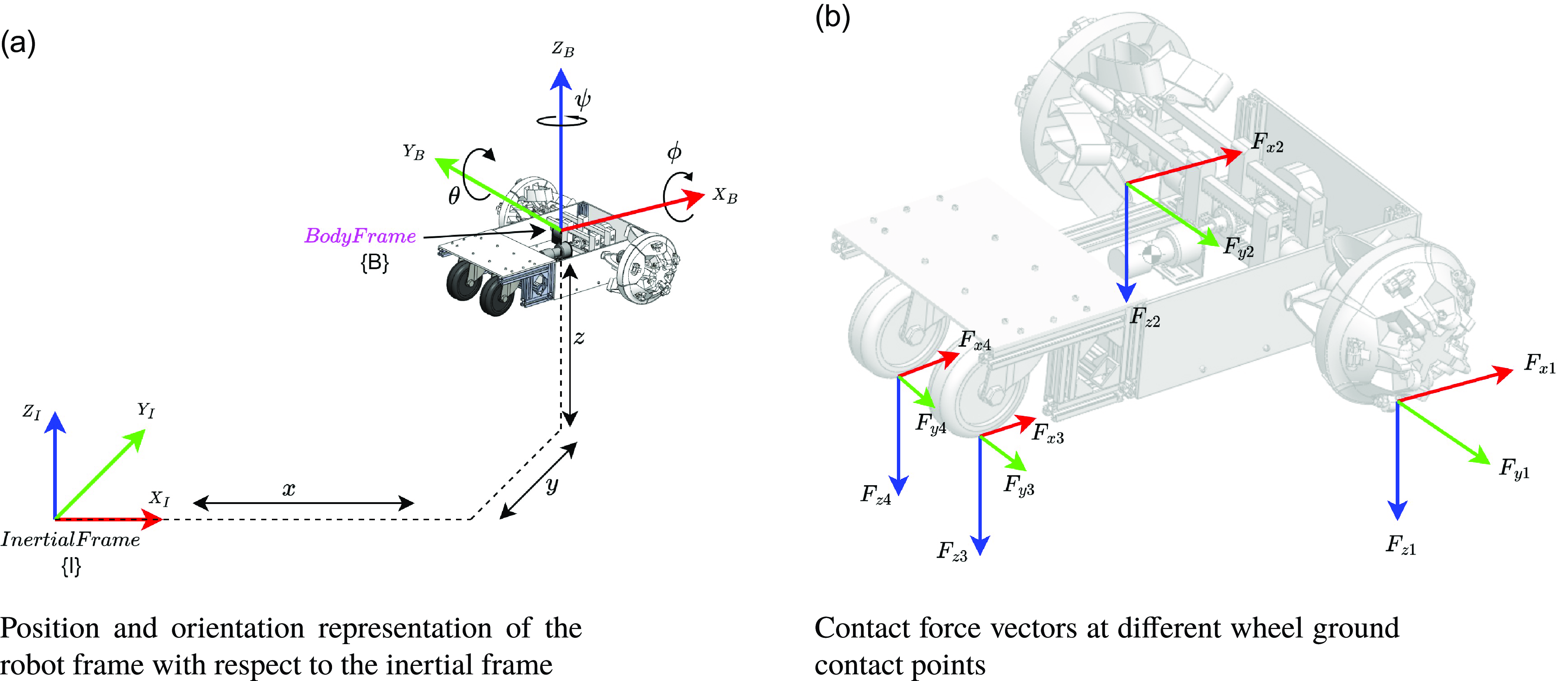
Position, orientation, and contact forces on the robot with respect to the Inertial frame.

Position and orientation of the robot body frame, with respect to the inertial frame, can be described by a vector,
 $\boldsymbol{\eta }=[x,y,z,\phi ,\theta ,\psi ]^{\text{T}}$
, as shown in Figure (12a). The linear and angular velocity vector of the robot is denoted by
 $\boldsymbol{\nu }=[u,v,w,p,q,r]^{\text{T}}$
. The vectors
 $\boldsymbol{\eta }$
and
 $\boldsymbol{\nu }$
are in the vector space
 ${\mathbb{R}}^{6}$
. Now the equation of motion for the robot can be written as:
 \begin{equation} {\mathbf {M}}\boldsymbol{\dot {\nu }}+{\mathbf {C}}(\boldsymbol{\nu })\boldsymbol{\nu }+{\mathbf {g}}(\boldsymbol{\eta })=\boldsymbol{\tau } \end{equation}
where
 ${\mathbf {M}}\in {\mathbb{R}}^{6X6}$
is the mass matrix,
 ${\mathbf {C}}(\boldsymbol{\nu })\in {\mathbb{R}}^{6X1}$
is the vector of centripetal and Coriolis forces,
 ${\mathbf {g}}(\boldsymbol{\eta }) \in {\mathbb{R}}^{6X1}$
is the gravity vector and
 $\boldsymbol{\tau }\in {\mathbb{R}}^{6X1}$
is the vector of input forces and moments on the robot, in body frame. From Eq. (49), the position and velocity of the robot obtained are in the body frame {B}, which needs to be mapped with respect to the inertial frame {I}. For this mapping, we need two transformation operators
 ${\mathbf {J}}_{1}({\boldsymbol{\eta _{2}}})$
for linear velocity transformation and
 $ {\mathbf {J}}_{2}(\boldsymbol{\eta _{2}})$
for angular velocity transformations, which are given below:
 \begin{equation} {\mathbf {J}}_{1}(\boldsymbol{\eta _{2}})=\begin{bmatrix} \cos {\psi }\cos {\theta } & -\sin {\psi }\cos {\phi }+\cos {\psi }\sin {\theta }\sin {\phi } & \sin {\psi }\sin {\phi }+\cos {\psi }\cos {\phi }\sin {\theta }\\[3pt] \sin {\psi }\cos {\theta } & \cos {\psi }\cos {\phi }+\sin {\phi }\sin {\theta }\sin {\psi } & -\cos {\psi }\sin {\phi }+\sin {\theta }\sin {\psi }\cos {\phi }\\[3pt] -\sin {\theta } & \cos {\theta }\sin {\phi } & \cos {\theta }\cos {\phi } \end{bmatrix} \end{equation}
 \begin{equation} {\mathbf {J}}_{2}(\boldsymbol{\eta _{2}})=\begin{bmatrix} 1 &\quad \sin {\phi }\tan {\theta } &\quad \cos {\phi }\tan {\theta }\\[3pt]0 &\quad \cos {\phi } &\quad -\sin {\phi }\\[3pt]0 &\quad \sin {\phi }/\cos {\theta } &\quad \cos {\phi }/\cos {\theta } \end{bmatrix} \end{equation}
In Eq. (49), the input vector is defined as
 $\tau =[F_{x},F_{y},F_{z},M_{x},M_{y},M_{z}]^{T}$
, where
 $F_{x}, F_{y},$
and
 $F_{z}$
represent the input forces along the
 $X, Y,$
and
 $Z$
axes, respectively, of the vehicle frame. Similarly,
 $M_{x}, M_{y}$
, and
 $M_{z}$
represent the moments around the
 $X$
,
 $Y$
, and
 $Z$
axes, respectively, of the vehicle frame. The equation of motion is defined in the robot’s body frame, which is situated at the vehicle’s COM. The force vector, including normal contact reaction, traction forces, and frictional forces, is located at the wheel and the ground contact frame and is in inertial frame {I}, but with a different orientation than the inertial frame. However, the moment vector is already computed with respect to the vehicle frame {B}, in the system dynamics section, and thus requires no further transformation. Therefore, before incorporating these contact forces into the
 $\boldsymbol{\tau }$
vector, it is necessary to transform them to the COM position or the body frame, via suitable transformations. In the present scenario, the contact force vector located at the wheel and ground contact frame will first be transformed to the Inertial frame using the required rotation matrices. After the force vector has been determined in the inertial frame, it can be transformed to the vehicle frame utilizing the
 ${\mathbf {J}}_{1}(\boldsymbol{\eta _{2}})$
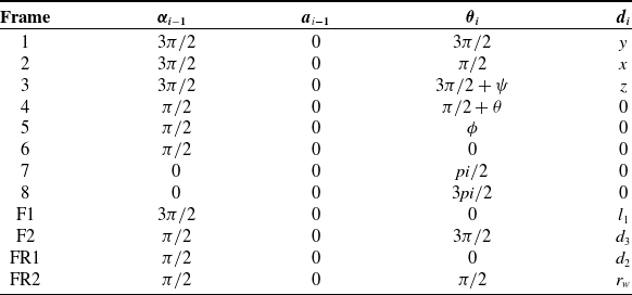
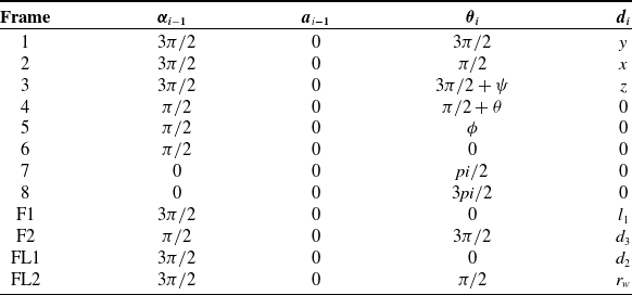
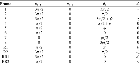
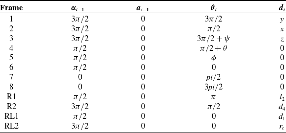
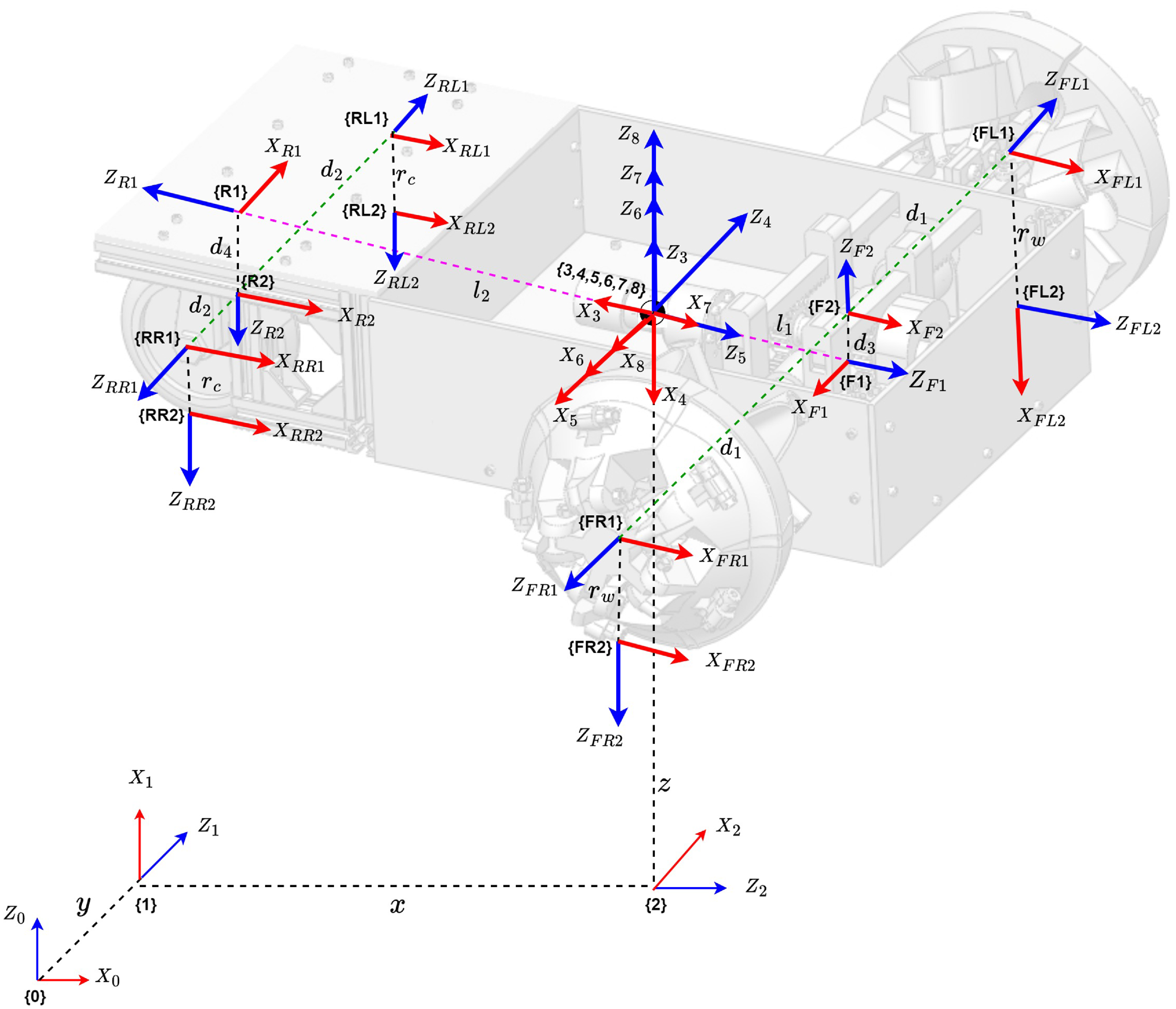
transformation function, as delineated in Eq. (50). Additionally, the rotation matrices required to transform force vectors from their respective contact frame to the inertial frame can be derived from the DH parameter Tables I, II, III, and IV, with the associated kinematic frame diagram illustrated in Figure 13.
DH Table for front right wheel.

DH Table for front left wheel.
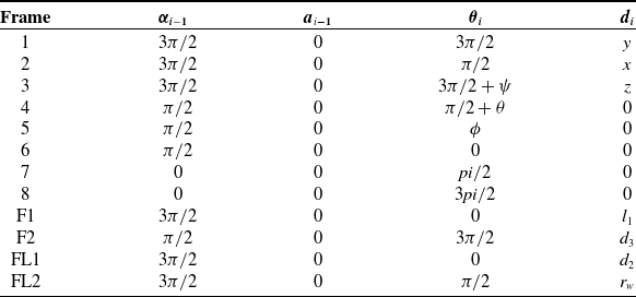
DH Table for rear right caster wheel.

DH Table for rear left caster wheel.

Kinematic frame diagram of the proposed robot.

Now since the contact frame of all four wheels, i.e. {FR2}, {FL2}, {RR2}, and {RL2} have the same orientation with respect to the body frame, which is frame {7} corresponding to the Figure 13. Therefore, the rotation matrix required to transform all four wheel contact frames with respect to the inertial frame (
 ${\mathbf {R}}_{w}^{I}$
) is given by Eq. (52).
 \begin{equation} {\mathbf {R}}_{w}^{I} = \begin{bmatrix} 1 &\quad 0 &\quad 0\\[3pt]0 &\quad -1 &\quad 0\\[3pt]0 &\quad 0 &\quad -1 \end{bmatrix} \end{equation}
Now, the components of the vector of input force with respect to the inertial frame can be computed as follows:
 \begin{equation} \begin{bmatrix} F_{x}\\[3pt]F_{y}\\[3pt]F_{z} \end{bmatrix}={\mathbf {R}}_{w}^{I}\begin{bmatrix} F_{x1}\\[3pt]F_{y1}\\[3pt]F_{z1} \end{bmatrix}+{\mathbf {R}}_{w}^{I}\begin{bmatrix} F_{x2}\\[3pt]F_{y2}\\[3pt]F_{z2} \end{bmatrix}+{\mathbf {R}}_{w}^{I}\begin{bmatrix} F_{x3}\\[3pt]F_{y3}\\[3pt]F_{z3} \end{bmatrix}+{\mathbf {R}}_{w}^{I}\begin{bmatrix} F_{x4}\\[3pt]F_{y4}\\[3pt]F_{z4} \end{bmatrix} \end{equation}
where
 \begin{equation} \begin{bmatrix} F_{x1}\\[3pt]F_{y1}\\[3pt]F_{z1} \end{bmatrix}=\begin{bmatrix} \frac {\tau _{m}}{r_{w}}-\mu _{x}{\mathbf {N}}_{FRW}\\[3pt]\mu _{y}{\mathbf {N}}_{FRW}\\[3pt] {\mathbf {N}}_{FRW} \end{bmatrix} \end{equation}
 \begin{equation} \begin{bmatrix} F_{x2}\\[3pt]F_{y2}\\[3pt]F_{z2} \end{bmatrix}=\begin{bmatrix} \frac {\tau _{m}}{r_{w}}-\mu _{x}{\mathbf {N}}_{FLW}\\[3pt]\mu _{y}{\mathbf {N}}_{FLW}\\[3pt] {\mathbf {N}}_{FLW} \end{bmatrix} \end{equation}
 \begin{equation} \begin{bmatrix} F_{x3}\\[3pt]F_{y3}\\[3pt]F_{z3} \end{bmatrix}=\begin{bmatrix} -\mu _{x}{\mathbf {N}}_{RRC}\\[3pt]\mu _{y}{\mathbf {N}}_{RRC}\\[3pt] {\mathbf {N}}_{RRC} \end{bmatrix} \end{equation}
 \begin{equation} \begin{bmatrix} F_{x4}\\[3pt]F_{y4}\\[3pt]F_{z4} \end{bmatrix}=\begin{bmatrix} -\mu _{x}{\mathbf {N}}_{RLC}\\[3pt]\mu _{y}{\mathbf {N}}_{RLC}\\[3pt] {\mathbf {N}}_{RLC} \end{bmatrix} \end{equation}
Utilizing Eqs. (54) through (57), in conjunction with Eq. (53), we can determine the necessary input force vector in the body frame as delineated in Eq. (58).
 \begin{equation} \begin{bmatrix} F_{x}\\[3pt]F_{y}\\[3pt]F_{z} \end{bmatrix}={\mathbf {J}}_{1}(\eta _{2})'\begin{bmatrix} \frac {2\tau _{m}}{r_{w}}-\mu _{x}({\mathbf {N}}_{FRW}+{\mathbf {N}}_{FLW}+{\mathbf {N}}_{RRC}+{\mathbf {N}}_{RLC})\\[3pt] -\mu _{y}({\mathbf {N}}_{FRW}+{\mathbf {N}}_{FLW}+{\mathbf {N}}_{RRC}+{\mathbf {N}}_{RLC})\\[3pt] {\mathbf {N}}_{FRW}+{\mathbf {N}}_{FLW}+{\mathbf {N}}_{RRC}+{\mathbf {N}}_{RLC} \end{bmatrix} \end{equation}
Similarly, we can articulate the input moment vector to the body frame as:
 \begin{equation} \begin{bmatrix} M_{x}\\[3pt]M_{y}\\[3pt]M_{z} \end{bmatrix}=\begin{bmatrix} d_{1}({\mathbf {N}}_{FLW}-{\mathbf {N}}_{FRW})-d_{2}({\mathbf {N}}_{RRC}-{\mathbf {N}}_{RLC})\\[3pt] -l_{1}({\mathbf {N}}_{FRW}+{\mathbf {N}}_{FLW})+l_{2}({\mathbf {N}}_{RRC}+{\mathbf {N}}_{RLC})-h(F_{x1}+F_{x2}-F_{x3}-F_{x4})\\[3pt] F_{x1}d_{1}-F_{x2}d_{1}-F_{x3}d_{2}+F_{x4}d_{2} \end{bmatrix} \end{equation}
In Eq. (59), if the system operates in wheel mode, we may use
 $l_{1}, l_{2}$
, and
 $h$
as specified in the equation. However, if the system is in legged mode, these lengths will be altered to
 $l_{1}^{\prime}, l^{\prime}_{2}$
, and
 $h'$
, as previously elucidated in Section 2. Additionally,
 $r_{w}$
denotes the radius of the front wheel, which varies across leg mode and wheel mode, i.e, 0.09 m in wheel mode and 0.16 m in legged mode. Additionally,
 $r_{c}$
denotes the radius of the caster wheel, whereas
 $\tau _{m}$
represents the motor torque supplied for propelling the front wheels.
5. Robot control
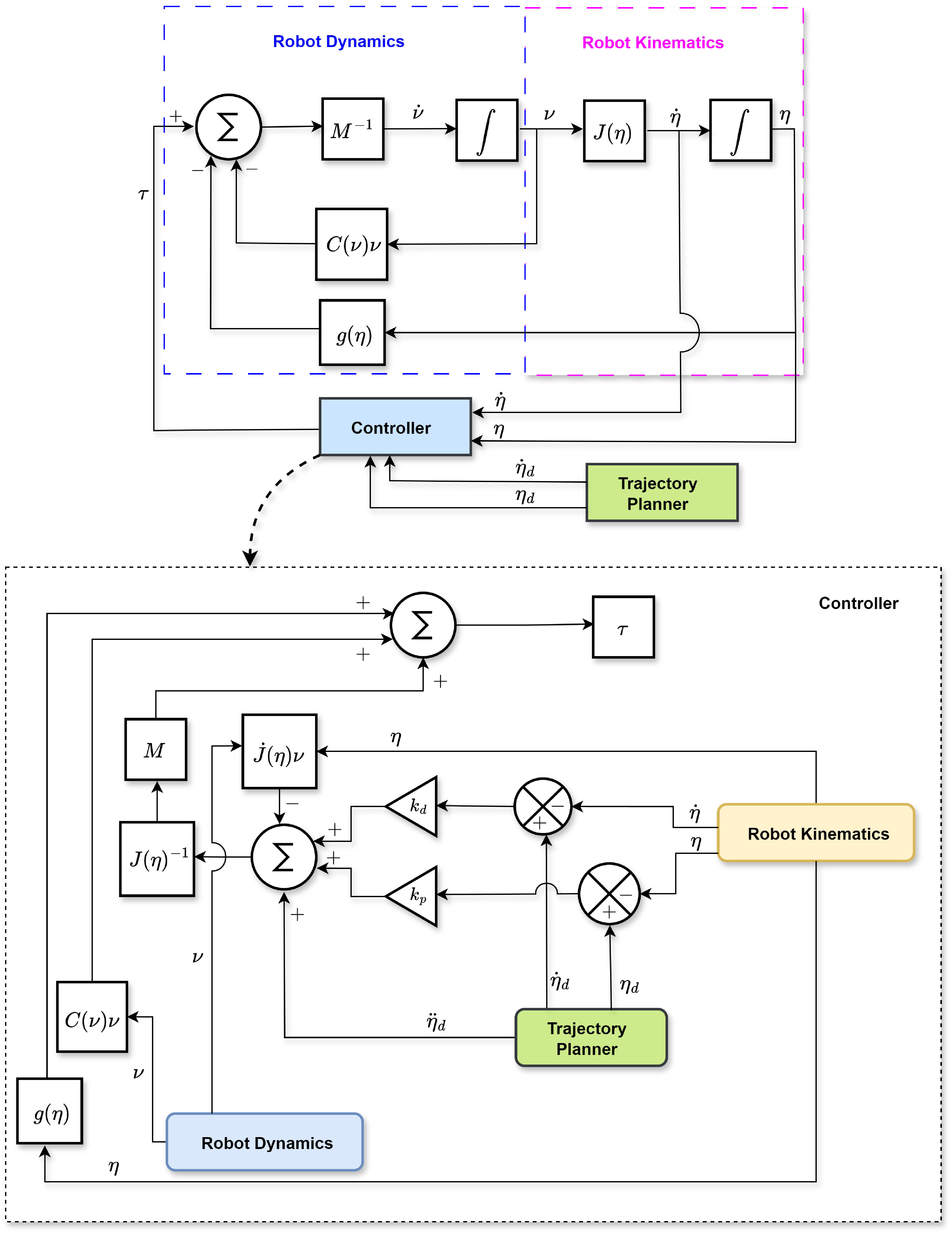
To examine the robot’s mobility, performance, and stability in various operating modes (legged or wheeled) over varied trajectories, a control plan must be developed to integrate with the system. This section will outline the control approach for managing the robot’s mobility over various trajectories. Moreover, this study primarily aims to examine the system’s dynamics under a certain control scheme, rather than to investigate the performance of many kinds of control systems on the robot [Reference Raikwar, Fehrmann and Herlitzius28–Reference Chen, Zhan, Jiang, Zhang, Rao, Wang and Li31]. Consequently, for this project, a computed input control system is used to control the motion of the robot, which fundamentally employs a Proportional Derivative (PD) control mechanism. To implement computed input control, it is assumed that the system exhibits exponential stability over time. Which means, as
 $ t \rightarrow \infty$
, it follows that
 $\boldsymbol{\tilde {\eta }} \rightarrow 0$
and
 $ \boldsymbol{\dot {\tilde {\eta }}} \rightarrow 0$
. where,
 $\boldsymbol{\tilde {\eta }}=\eta _{\text{desired}}-\eta _{\text{actual}}$
and
 $\boldsymbol{\dot {\tilde {\eta }}}=\dot {\eta }_{\text{desired}}-\dot {\eta }_{\text{actual}}$
. From the second-order error dynamic model, the basic error model can be articulated as:
 \begin{equation} \ddot {\boldsymbol{\eta }}+k_{d}\dot {\tilde {\boldsymbol{\eta }}}+k_{p}\tilde {\boldsymbol{\eta }}=0 \end{equation}
where
 $k_{p}\gt 0$
and
 $k_{d}\gt 0$
are the constants of proportional and derivative gains, respectively. However, these two are positive definite diagonal matrices, but for simplicity, they are represented as scalars here.
 \begin{equation} \ddot {\boldsymbol{\eta }}_{d}-\ddot {\boldsymbol{\eta }}+k_{d}\dot {\tilde {\boldsymbol{\eta }}}+k_{p}\tilde {\boldsymbol{\eta }}=0 \end{equation}
 \begin{equation} \ddot {\boldsymbol{\eta }}=\ddot {\boldsymbol{\eta }}_{d}+k_{d}\dot {\tilde {\boldsymbol{\eta }}}+k_{p}\tilde {\boldsymbol{\eta }} \end{equation}
but,
 \begin{equation} \ddot {\eta }={\mathbf {J}}(\boldsymbol{\eta })\dot {\boldsymbol{\nu }}+\dot {\mathbf {J}}(\boldsymbol{\eta })\boldsymbol{\nu } \end{equation}
and,
 \begin{equation} \dot {\boldsymbol{\nu }}={\mathbf {J}}^{-1}(\boldsymbol{\eta })[\ddot {\boldsymbol{\eta }}-\dot {\mathbf {J}}(\boldsymbol{\eta })\boldsymbol{\nu }] \end{equation}
using Eq. (49) we can write Eq. (64) as:
 \begin{equation} {\mathbf {M}}^{-1}[\boldsymbol{\tau } - {\mathbf {C}(\boldsymbol{\nu })\boldsymbol{\nu } + {\mathbf {g}}(\boldsymbol{\eta })}] = {\mathbf {J}}^{-1}(\boldsymbol{\eta })[\ddot {\boldsymbol{\eta }}-\dot {\mathbf {J}}(\boldsymbol{\eta })\boldsymbol{\nu }] \end{equation}
and now using Eq. (62) and (65), input vector
 $\tau$
can be written as:
 \begin{equation} \boldsymbol{\tau } = {\mathbf {M}}{\mathbf {J}}(\boldsymbol{\eta })^{-1}[\ddot {\boldsymbol{\eta }}_{d} + k_{d}\dot {\tilde {\boldsymbol{\eta }}} + k_{p}\tilde {\boldsymbol{\eta }}-\dot {\mathbf {J}}(\boldsymbol{\eta })\boldsymbol{\nu }]+ [{\mathbf {C}}(\boldsymbol{\nu })\boldsymbol{\nu } + {\mathbf {g}}(\boldsymbol{\eta })] \end{equation}
Eq. (66) represents the necessary control input supplied by the controller to the robot dynamics block, corresponding to the Figure 14, which illustrates a comprehensive control architecture. In this context, the forward dynamics is used to compute the system’s acceleration, which is then utilized by kinematics to determine the system’s position and orientation. The trajectory planner block supplies the intended position and orientation vector, in addition to the desired velocity and acceleration vector. The controller block computes the positional and velocity error, and using the corresponding
 $k_{p}$
and
 $k_{d}$
gains, it determines the necessary torque vector, which is then fed to the robot dynamics block, therefore completing the loop.
Control scheme of the robot.

6. System design and integration
This section addresses the system’s physical design. The robot design is developed using SolidWorks 2019 software, as seen in Figure 2. The robot comprises a total of four wheels: two passive caster wheels positioned at the back and two reconfigurable powered wheels situated at the front. The wheel reconfiguration employs a slider crank mechanism coupled with a rack and pinion arrangement on both front wheels. Three motors are used on the actuator side, two for operating the front wheels and one for triggering the reconfiguration mechanism. The primary chassis of the robot consists of 20 mm
 $\times$
20 mm aluminum profiles and 4 mm thick transparent acrylic sheets, as seen in Figure 1. The robot is equipped with two reconfigurable wheels and two standard caster wheels. The reconfigurable wheel consists of five sets of slider-crank mechanisms, functioning as the spokes of the wheel. These reconfigurable wheels are produced using 3D printing with PLA material. The reconfiguration mechanism of both wheels is connected to the reconfiguration motor via a rack and pinion assembly, which is fabricated using 3D printing technology. The robot comprises four racks and two pinions, with one pinion and two racks allocated to each wheel. Additional minor components, such as bearing holders and rack clamps, are also produced by 3D printing. The ESP-32 microcontroller serves as the primary controller for robot operation. To operate the robot, two 12V, 30 RPM DC geared motors equipped with encoders (Johnson motors from Orange company) are used. A 12V, 20 RPM DC geared motor (Johnson motor from Orange company) serves as the reconfiguration motor. Two CYTRON MDD3A motor driver boards are used to regulate the energy requirements of the motors and a 10,000 mAh Li-ion battery is used to power the robot. The robot utilizes micro-ROS for control, and the IMU MPU6050 is used for collecting accelerometer and gyroscopic data for determining the robot’s position. Following the assembly of all components into a final reconfigurable wheeled robot, it was evaluated inside the college campus in both wheel and legged modes across various indoor and outdoor environments, whose testing video is available at this link.
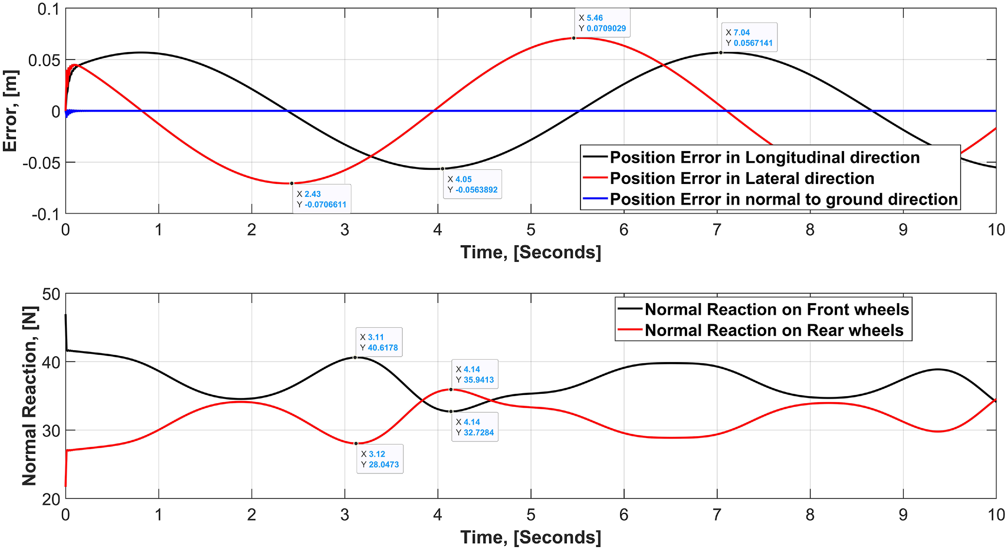
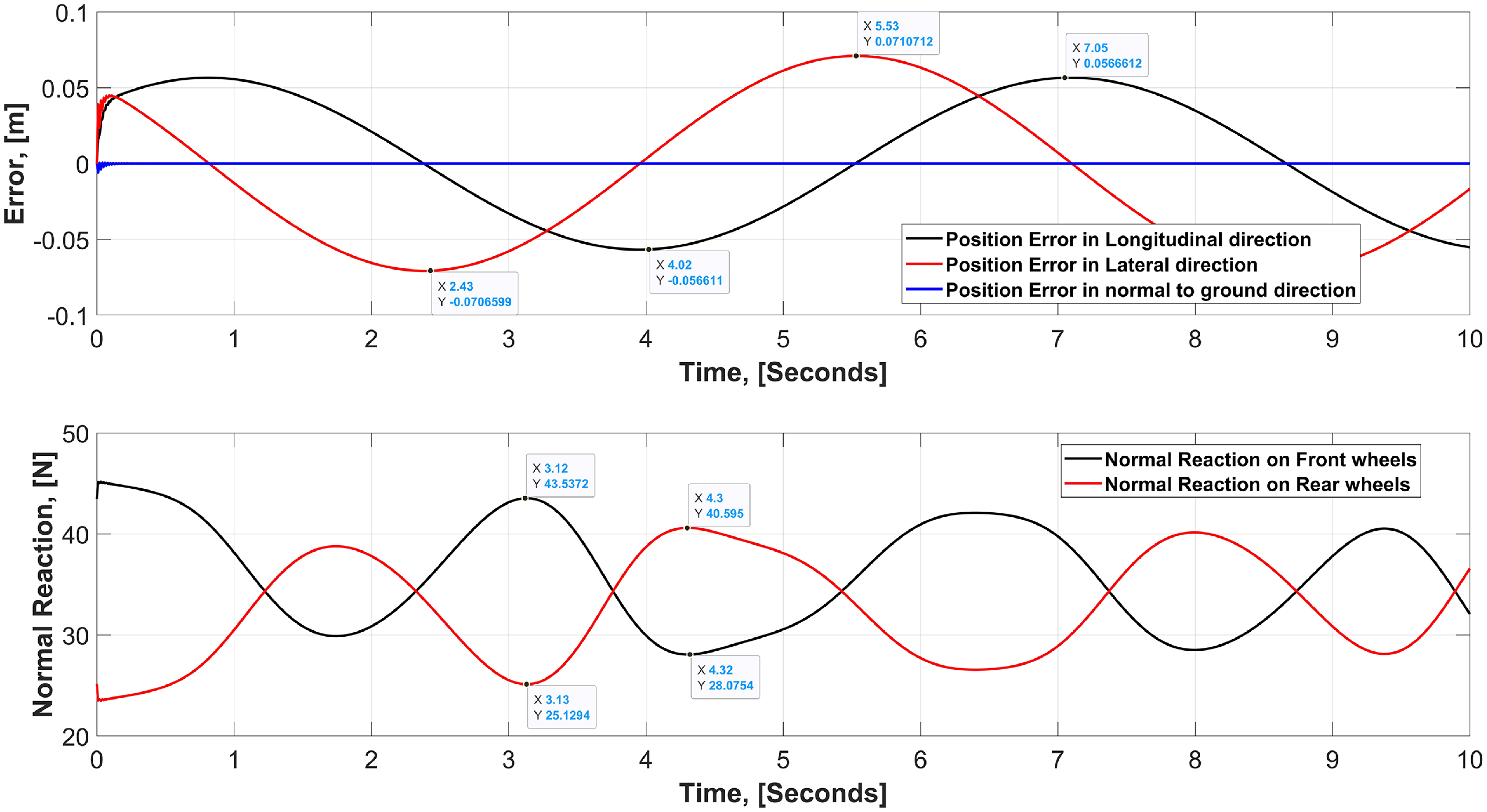
Temporal variation in normal reaction (bottom) and positional error (top) in wheel mode of longitudinal dynamics.

7. Results and discussion
This section will examine the robot’s stability and performance across various terrains and circumstances. In Section 2, we addressed the longitudinal dynamics, which encapsulate the impact of the robot’s pitching. Likewise, in lateral dynamics, we aimed to quantify the impact of the robot’s rolling on the normal reaction force exerted on various wheels of the system. Consequently, this part will demonstrate the system’s stability and the variation of normal reaction in both wheel mode and legged mode for longitudinal and lateral dynamics. Moreover, the force and torque required by the reconfiguration motor, discussed in the reconfiguration dynamics section, are also integrated into the program to assess the torque required by the reconfiguration motor under varying normal reaction on the wheels. All these findings are derived from the numerical simulation conducted using the MATLAB 2021b program.
7.1. Performance in longitudinal dynamics
7.1.1. Wheel mode
A helical trajectory (
 $[2\sin {t}, 2\cos {t}, 0.5t]^{\text{T}}$
) is selected for the assessment of the robot’s performance and stability in numerical simulation. Furthermore, to ensure the robot’s adherence to the specified trajectory, the computed input controller, as elaborated in Section 5, is used. The upper section of Figure 15 illustrates the positioning inaccuracy across all three dimensions: longitudinal, lateral, and vertical, with time. The robot demonstrates stability within 0.25 s of simulation time, exhibiting a positional error ranging from 0 to
 $\pm$
7 cm in the lateral and 0 to
 $\pm$
5.6 cm in longitudinal directions along with 0 to
 $\pm$
1 mm in the vertical direction. This error arises primarily from the centrifugal force exerted on the robot laterally during motion, causing the robot to drift outward owing to both the centrifugal force and the fluctuating sinusoidal trajectory over time. Second, rear wheels are passive casters and are free to rotate about their steering axis, due to which, during curved trajectory, these casters always create deviation and lateral drift in the robot’s overall motion. Additionally, due to the caster’s free motion about their steering axis, initially, when the robot’s controller starts controlling its motion, these casters take some time to get aligned with the active front wheel’s motion, and hence contribute in creating chattering at the beginning of the motion. Once these casters are aligned with the front wheel’s motion, then this chattering disappears automatically.
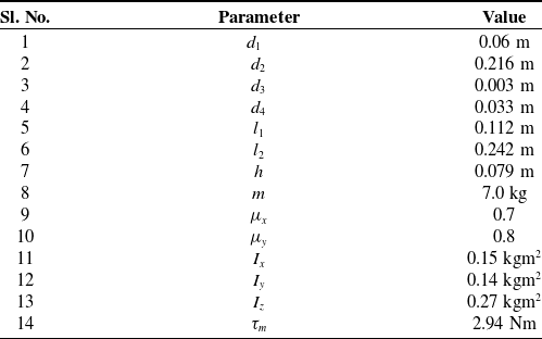
Likewise, the lower section of the picture illustrates the temporal variation of the normal reaction on the front and rear wheels. The longitudinal dynamic analysis of the robot presumes that the normal reaction on the front two wheels is uniform, as is the case for the rear two wheels. Consequently, just the variation of front and rear wheels is shown here. The primary observation is that the normal reaction on the rear wheels is consistently less than that on the front wheels for the whole simulation period, except few instances. This is attributable to the position of the COM toward the front axle, denoted as the distance
 $l_{1}$
in Table V. Secondly, it is evident that the controller is rectifying any positional drift of the robot in both longitudinal and lateral directions; nonetheless, this positional drift results in a change of the normal reaction curve throughout.
Robot’s physical and other parameters used in the simulation.

Reconfiguration mechanism’s physical parameters.

Position error (top) and normal reaction (bottom) variation with time in leg mode of longitudinal dynamics.

7.1.2. Leg mode
In leg mode, the COM of the system shifts along both the length and height of the robot’s body. Due to the rear wheels being casters and having a smaller diameter than the front wheels, the robot’s body is somewhat tilted toward the rear axle in leg mode. As a result of a rotation of
 $10.2^{\circ }$
around the contact point of the rear caster with the ground. This tilt results from the transition from wheel mode to leg mode. The top part of Figure 16 illustrates the positional inaccuracy across all three axes of the inertial frame as a function of time, while the lower section depicts the change in normal reaction forces on the front and rear wheels over time. Under leg mode, the error stabilizes once again after 0.25 s of simulation time. In the vertical direction, there is no inaccuracy after 0.1 s. The inaccuracy in the longitudinal direction ranges from 0 to
 $\pm 5.6$
cm, and in lateral direction it is 0 to
 $\pm 7$
cm after 1 s of simulation time. This error is again owing to the free movement of casters about the steering axis, centrifugal force, and a sinusoidal trajectory. It is also crucial to acknowledge that the shifting of the COM toward the geometric center of the robot’s body and the change in moment of inertial tensor of the overall system due to reconfiguration have resulted in increased normal reaction on the rear wheels in leg mode, compared to wheel mode, as shown in the bottom part of Figure 16. In wheeled mode, average normal reaction on the front and rear wheels was 37.15 N and 31.51 N, which in legged mode is 36.01 N and 32.64 N, respectively. This increase in normal reaction on the rear wheel and decrease in normal reaction on the front wheel due to the reconfiguration is approximately 3.46% variation, hence justifies the longitudinal dynamics formulation as described for the normal reactions in the system dynamics section.
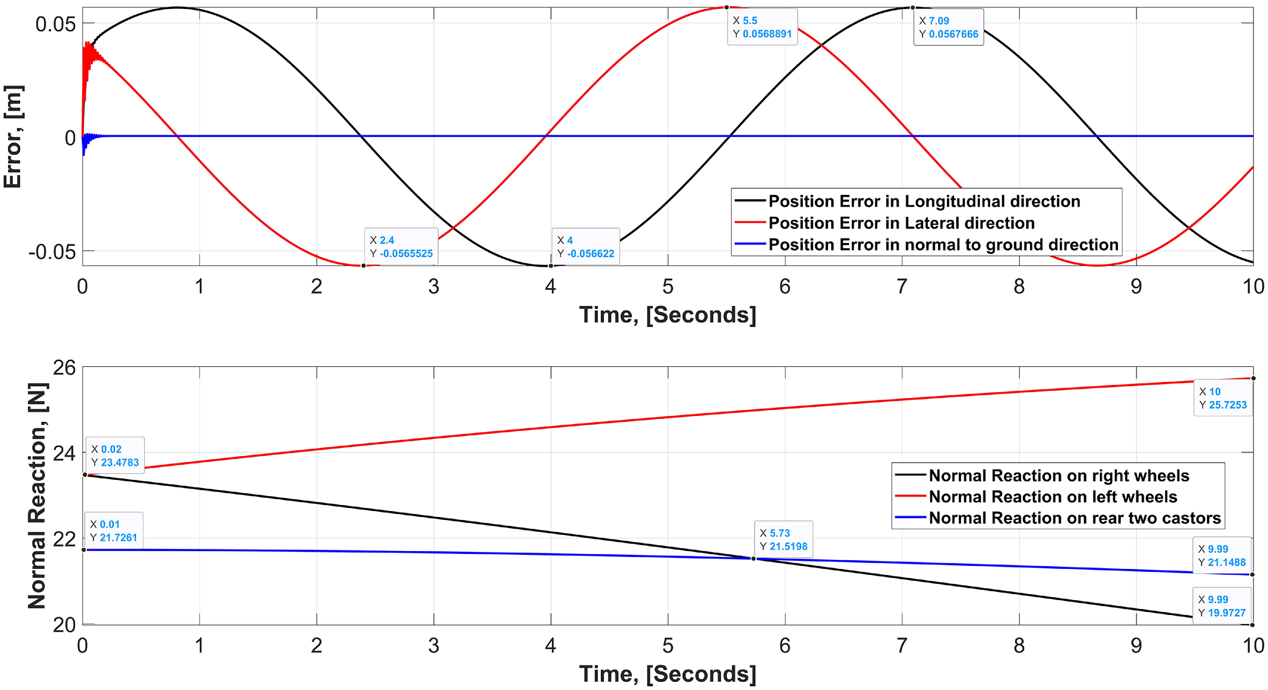
Position error and normal reaction variation with time in wheel mode of lateral dynamics.

7.2. Performance in lateral dynamics
7.2.1. Wheel mode
For lateral dynamics, the system is approximated as the tricycle model, as discussed in the system dynamics section, in which the rear two casters will have the same normal reaction. Now, referring to Figure 17, it is evident that the robot achieves stabilization around 0.25 s of the simulation time, with a maximum lateral and longitudinal positional error ranging from 0 to
 $\pm 5.6$
cm only. Conversely, an examination of the variation in the normal reaction force on the right and left side wheels, as depicted in the lower section of Figure 17, reveals that the left side wheels, or outer wheels, experience a greater normal reaction force than the inner wheels, or right side wheels, due to the influence of centrifugal force. In the simulation, a constant acceleration acts on the system, resulting in a continual increase in the normal reaction on the left wheel and a continuous decrease in the normal reaction of the right wheel. Nonetheless, the robot will remain upright, provided that both the right and left wheels get a positive normal reaction force from the ground. The average normal reaction on the front right and front left reconfigurable wheel is 21.76 N and 24.74 N, respectively. Additionally, the normal reaction on the rear two casters jointly is about 24.98 N in wheel mode. Now, it is evident that due to the rolling motion of the robot about it’s X-axis of the vehicle frame, left and right wheels are experiencing different normal reaction, while on rear casters, magnitude of the reaction is between the reaction on left and right wheel, hence, justifies our tricycle approximation for lateral dynamics satisfactorily.
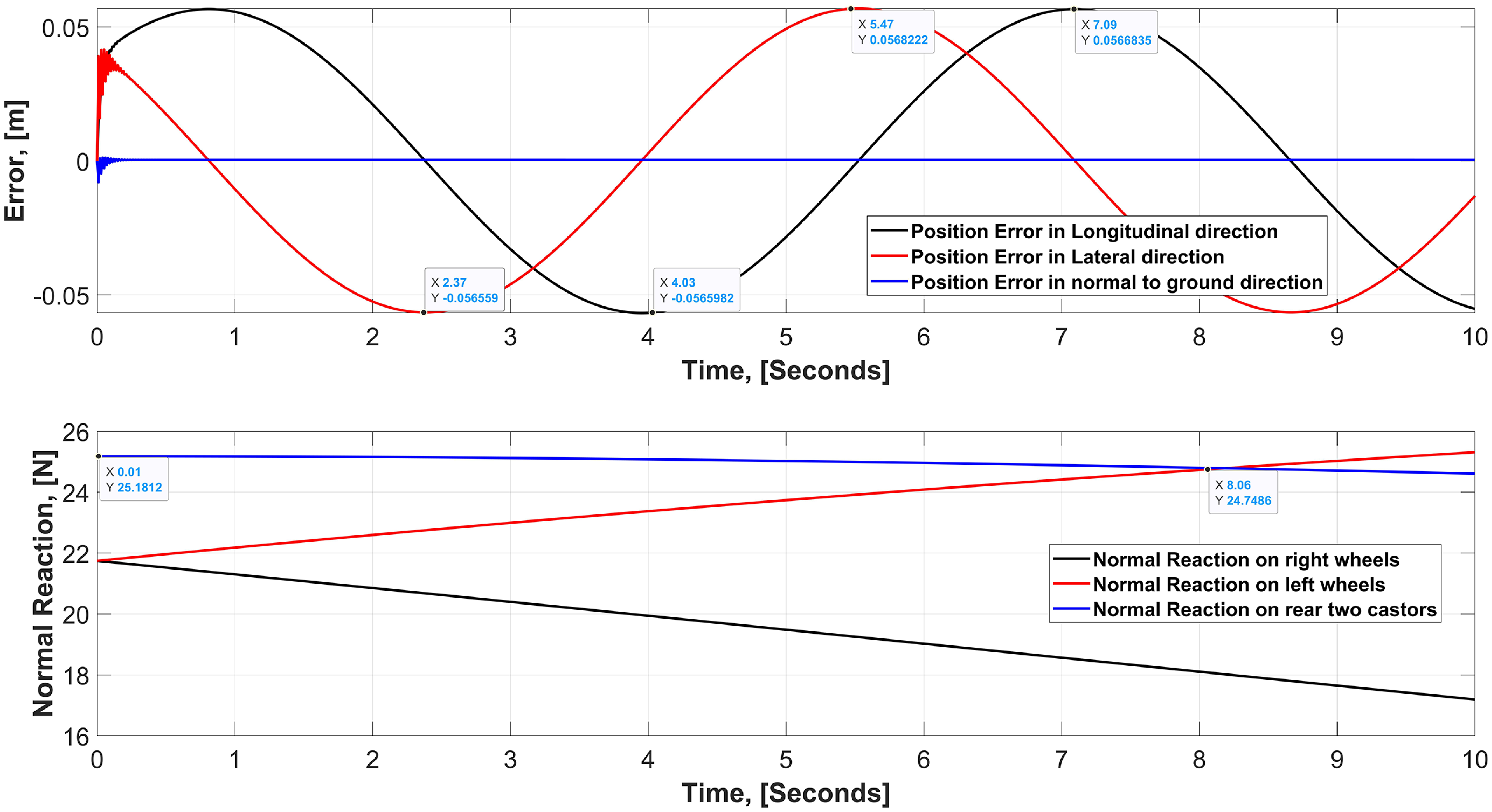
Position error and normal reaction variation with time in leg mode of lateral dynamics.

7.2.2. Leg mode
When the front left and right wheels of the robot are transformed into leg mode, the COM shifts within the X-Z plane of the robot’s frame, along with changes in the moment of inertia of the overall system. In lateral dynamics, only the elevation of the COM and the change in moment of inertia of the system influence the transition from wheel mode to legged mode. The impact of rotation about the x-axis is seen in the lower section of Figure 18, which also depicts the body roll in the robot. The normal reaction on the outer wheels, or left wheels, exceeds that on the inner wheels, or right wheels, owing to the influence of centrifugal force. Ground reaction force on the front right wheel and front left wheel is 19.47 N and 23.67 N, respectively, while on the rear two casters together it is about 24.98 N. This variation in normal reaction on inner and outer wheel is about 17.7% in the legged mode, while it was only 12% in the wheel mode. This discrepancy arises from the elevated COM of the robot, boosting the moment’s magnitude around the X-axis under rolling conditions.
Variation of motor torque in longitudinal dynamics.

7.3. Reconfiguration motor torque variation in longitudinal and lateral dynamics
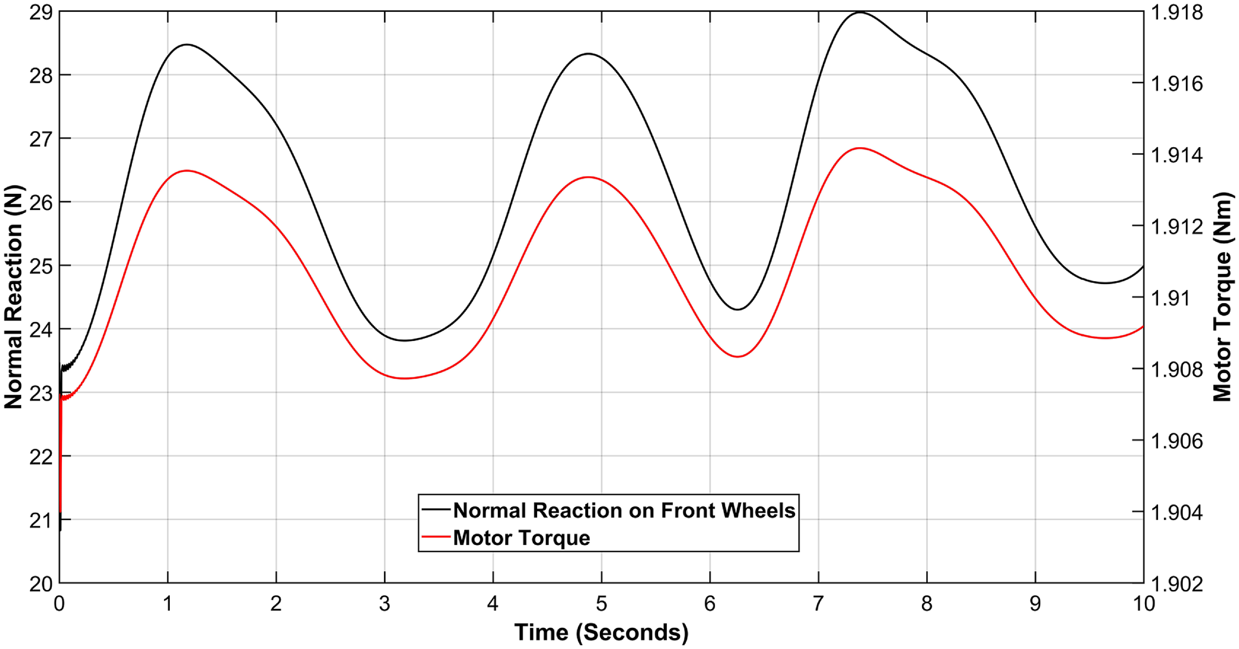
In Section 3, we analyzed the dynamics of the reconfiguration mechanism used in the robot’s front two wheels, using Eq. (48) alongside Eq. (29). This dynamic analysis estimates the torque required at the motor end, aiding in the selection of a suitable off-the-shelf motor. Now, reconfiguration of the wheel may be required at any point while the robot is in motion. Therefore, it is important to evaluate the maximum normal reaction imparted to the robot’s wheel during motion while selecting any actuator. Nonetheless, the normal reaction varies in accordance with the vehicle’s lateral and longitudinal dynamics, alongside the designated trajectory. Consequently, to include each of these aspects in the motor selection process, the motion of robots must be analyzed in both wheeled and legged configurations under longitudinal and lateral dynamic conditions. Therefore, under longitudinal dynamic conditions, from Figure 19, it is evident that the motor torque fluctuates over time in response to the fluctuation of the normal reaction on the transformable front wheel. From the same figure, it is also observed that the motor requires an average torque of 1.9 Nm to achieve a linear acceleration of 1 m/s2 on the slider, with a lateral coefficient of friction of 0.8 between the leg and the ground.
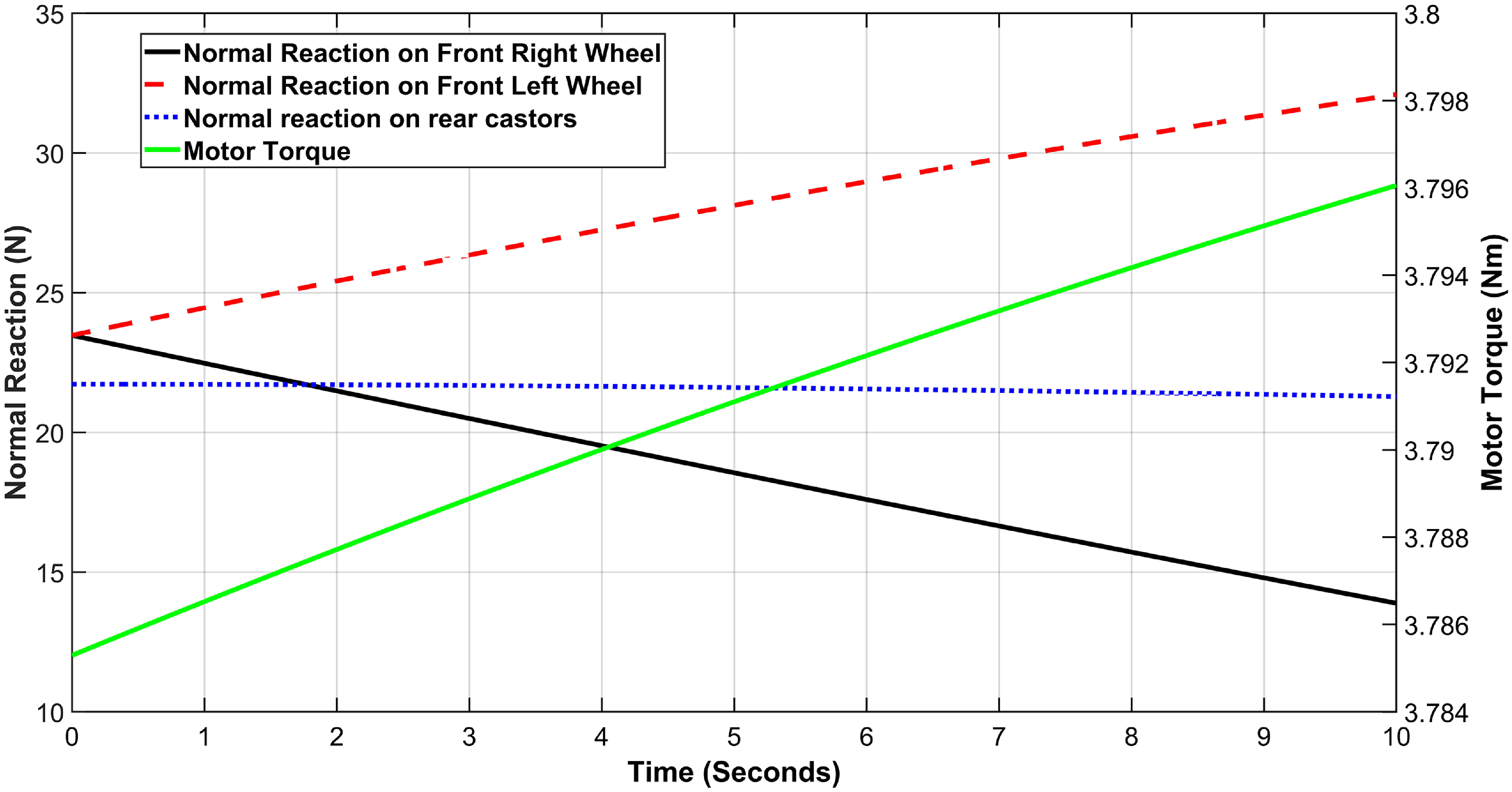
Likewise, Figure 20 illustrates the fluctuation of motor torque under lateral dynamics scenarios. The torque exhibits a small variation, with an average value of 3.7 Nm. Upon analyzing the torque requirements of the reconfiguration motor under lateral and longitudinal dynamic situations, it is essential to pick a motor capable of delivering a minimum torque of 3.7 Nm, which corresponds to a linear acceleration of 1 m/s2 and a reconfiguration duration of 2 s.
Variation of motor torque in lateral dynamics.

Actual robot in leg-mode.

8. Conclusion and future work
This study examines a reconfigurable, wheeled-legged, four-wheeled mobile robot. This robot is designed for outdoor, unstructured terrain; the front two wheels are adjustable, while the back two wheels are casters. Each reconfigurable wheel has five sets of slider-crank mechanisms to facilitate the transition from wheel mode to leg mode. To guarantee the robot’s stability in an unstructured environment, dynamic analyses of lateral and longitudinal movements are conducted in both wheel and legged modes. This analysis assists the controller in delivering the necessary input for the robot’s steady movement over uneven terrain. For the chosen helical trajectory, the positioning error is within
 $\pm$
7 cm, which is satisfactory as per the size of the robot. The reconfiguration dynamics and system dynamics together facilitated the selection of the motor necessary for wheel reconfiguration, as well as the motor needed for propulsion. According to the mathematical study, the motor must provide a minimum torque of around 3.7 Nm to achieve an acceleration of 1 m/s2 over a reconfiguration time of 2 s. However, in the actual system, the motor used for reconfiguration is capable of delivering a torque of 2.9 Nm, which is approximately the average torque of the lateral and longitudinal dynamic case, i.e, 2.8 Nm. Additionally, in a real robot, acceleration of 1 m/s2 is not desired, as it was initially developed for an undulated environment, where the robot’s stability is more crucial than agility. Furthermore, the robot components are constructed using PLA material just for testing purposes, which is inadequate for high-torque actuators. However, if the robot’s components are manufactured with light and robust materials like carbon fibr and aluminum alloys, then 3.9 Nm torque actuators may be employed. In future endeavors, all four wheels of the robot may be designed as reconfigurable kinds. Given that the current study focuses on the whole motion and dynamics of the system, future research might include testing the performance of the wheel on various obstacles across diverse real-world terrain conditions.
Author contributions
Mathematical modeling and article writing are done by Prashant Raturi. The hardware integration and testing of the robot are done by Shivansh Chaudhary. The conceptualization of the design and the overall direction of the project and the paper is done by Professor Santhakumar Mohan.
Financial support
This research was partially supported by the IIT Palakkad Technology IHub Foundation [Grant no: IPTIF/IP/09] and Anusandhan National Research Foundation [Grant no: CRG/2023/004646].
Competing interest
There is no conflict of interest among the authors.
Ethical approval
Not applicable in this work.