

1. Introduction
1.1 Frequentist statistics as model-based inference
Fisher’s (Reference Fisher1922) model-based statistics was a revolutionary recasting of Karl Pearson’s data-driven descriptive statistics (Yule Reference Yule1916) into modeling the stochastic mechanism that gave rise to the data
 ${{\bf{x}}_0}: = ({x_1},{x_2},...,{x_n})$
in the form of a parametric statistical model, generically specified as:
 $${{\cal M}_\theta }({\bf{x}}) = \{ f({\bf{x}};{\bf{\theta }}),\;{\bf{\theta }} \in \Theta \subset {{\mathbb R}^m}\} ,\;{\bf{x}} \in {\mathbb R}_X^n,\;n \gt m,$$
where
 $f({\bf x};{\bf\theta }),\ {\bf x}\mathit{\in }\mathbb{R}_{X}^{n}$
denotes the joint distribution of the sample
 ${\bf{X}}: = {\bf{(}}{X_1}, \ldots ,{X_n}{\bf{),}}$
 $\mathbb{R}_{X}^{n}$
denotes the sample space, and
 $\Theta $
the parameter space.
 ${{\cal M}_\theta }({\bf{x}})$
is chosen with a view to account for all the chance regularities in data
 ${{\bf{x}}_0}$
(see Spanos Reference Spanos2013a).
Example 1 The simple Normal model is specified by:
 $${{{{\cal M}_\theta }({\bf{x}}){\rm{:}}\,{{\rm{X}}_t}{\rm\sim NIID}(\mu ,{\sigma ^2}),{x_t} \in {\mathbb R},E({X_t}) = \mu \in {\mathbb R},Var({X_t}) = {\sigma ^2} \gt 0,\,t = 1,2,..,n, \ldots ,}}$$
where
 ${\rm{NIID}}$
stands for Normal, Independent, and Identically Distributed with mean
 $\mu $
and variance
 ${\sigma ^2}$
, which denote the probabilistic assumptions comprising (1).
The model-based approach to statistics began with Fisher (Reference Fisher1922, Reference Fisher1925) providing—almost single-handedly—an optimal theory of point estimation (see Hald Reference Hald2007). Neyman and Pearson (N-P) (Reference Neyman and Pearson1933) supplement that with the N-P theory of optimal testing by reformulating Fisher’s significance testing, and Neyman (Reference Neyman1937) provided an optimal theory of confidence intervals. The Fisher-Neyman-Pearson (F-N-P) paradigm has dominated modern frequentist statistics since the 1930s, but it has been plagued by several issues/problems:
[a] abuses/misapplications/misinterpretations of inferential procedures/results, such as p-hacking, multiple testing, cherry-picking, low-power studies, statistical misspecification, poor implementation of inference procedures, and unwarranted evidential interpretations of testing results (p-value, accept/reject
 ${H_0}$
), and
[b] genuine foundational problems, such as “the large (small) n problem,” establishing the statistical adequacy (the validity of the probabilistic assumptions comprising
${{\cal M}_\theta }({\bf{x}})$
(Spanos Reference Spanos1986), and a sound evidential interpretation of testing results.


These issues and problems have bedeviled the proper implementation of frequentist inference since the 1930s. Unfortunately, the current literature on the replication crisis often conflates [a] and [b], giving rise to additional confusions (see Ioannidis Reference Ioannidis2005). One of the aims of the discussion that follows is to distinguish clearly between [a] and [b] and explain how the error-statistical perspective on frequentist statistics can shed light on both.
1.2 Error statistics: A brief summary
In an attempt to address the statistical adequacy of
 ${{\cal M}_\theta }({\bf{x}})$
, error statistics refines the F-N-P approach to frequentist inference by separating the modeling from the inference facet. The modeling facet includes estimation, misspecification testing, and respecification in order to secure the statistical adequacy of
 ${{\cal M}_\theta }({\bf{x}}),$
before the inference facet, where one poses substantive questions of interest to the data (see Mayo and Spanos Reference Mayo and Spanos2004, Spanos Reference Spanos2018). In an attempt to address the evidential interpretation of testing results, error statistics extends the F-N-P approach by distinguishing between predata and postdata facets of frequentist testing with a view to supplement the original framing with a postdata severity evaluation of testing results to provide a sound evidential account (see Mayo Reference Mayo1996, Mayo and Spanos Reference Mayo and Spanos2006, Reference Mayo, Spanos, Gabbay, Thagard and Woods2011).
The paper focuses primarily on Rochefort-Maranda (Reference Rochefort-Maranda2020) calling into question the cogency of the postdata severity evaluation when practitioners use underpowered tests. It is argued that this is a case of conflating [a] with [b] above. Unpacking this argument has broader ramifications since it reveals several fundamental misconceptions, which are broadly held in the current literature on the replication crisis.
Section 2 discusses the question of what constitutes trustworthy evidence and how to secure it. Section 3 revisits Rochefort-Maranda’s (Reference Rochefort-Maranda2020) numerical example with a view to demonstrate the difference between trustworthy and untrustworthy evidence stemming from misapplying frequentist testing. Section 4 considers the claim that “the more powerful the test the better the evidence against the null.” Section 5 discusses the difference between estimation-based effect sizes and testing-based effect sizes and calls into question the trustworthiness of the former.
2. Frequentist testing and trustworthy evidence
2.1 Power and the large n problem
As a prelude to the discussion that follows, consider testing the hypotheses:
 $$\matrix{ {{H_0}{\rm{:}}\ \mu \le {\mu _0}\ {\rm{vs}}\ {\rm{.}}{H_1}{\rm{:}}\ \mu \gt {\mu _0},} \cr } $$
in the context of the simple Normal model in (1). An
 $\alpha $
-significance level Uniformly Most Powerful (UMP) test is defined by (Lehmann and Romano Reference Lehmann and Romano2005):
 $$\matrix{ {{T_\alpha }: = \{ \tau ({\bf{X}}) = {{\sqrt n ({{\overline X }_n} - {\mu _0})} \over s},\;{C_1}(\alpha ) = \{ {\bf{x}}{\rm{:}}\ \tau ({\bf{x}}) \gt {c_\alpha }\} \} ,} \cr } $$
where
 ${c_\alpha }$
is the
 $\alpha $
-significance level threshold based on a Student’s t distribution with
 $(n - 1)$
degrees of freedom (St
 $(n - 1)$
):
 $\mathbb{P}(\tau (\mathbf{X})\gt c_{\alpha };\ \mu \ \mathit{=}\ \mu _{0})\mathit{=}\ \alpha ,\ $
based on the central Student’s t distribution:
 $$\matrix{ {\tau ({\bf{X}}) = {{\sqrt n ({{\overline X }_n} - {\mu _0})} \over s}\mathop \sim \limits^{\mu \, = \, {\mu _0}} {\rm{St}}(n - 1).} \cr } $$
The power of
 ${T_\alpha }$
, defined by:
 $$\mathcal{P}(\mu _{1})\,\mathit{=}\,\mathbb{P}(\tau (\mathbf{X})\gt c_{\alpha };\ \mu \, \mathbf{=}\, \mu _{1}),\,{\rm{for \ all}}\ \mu _{1}\mathbf{\gt}\mu _{0},$$
is based on the noncentral Student’s t distribution:
 $$\matrix{ {\tau ({\bf{X}}) = {{\sqrt n \left( {{{\overline X }_n} - {\mu _0}} \right)} \over s}\mathop \sim \limits^{\mu \,= \,{\mu _1}} {\rm{St}}({\delta _1};n - 1),\;{\delta _1} = {{\sqrt n \left( {{\mu _1} - {\mu _0}} \right)} \over \sigma },{\rm{for \ all}}\ {\mu _1}\!{\bf{ \gt }}\!{\mu _0},} \cr } $$
where
 ${\delta _1}$
is the noncentrality parameter (see Lehmann and Romano Reference Lehmann and Romano2005).
The predata role of power. As emphasized by Neyman (Reference Neyman1952) and Cohen (Reference Cohen1988), inter alia, the proper implementation of N-P testing requires one to use the (predata) power to determine the appropriate choice of the sample size n needed to ensure that test
 ${T_\alpha }$
has sufficient capacity, say
 $0.8$
, to detect discrepancies of interest
 ${\gamma _1}$
by solving for n in
 ${\delta _1} = {{\sqrt n \left( {{\mu _1} - {\mu _0}} \right)} \over \sigma }$
the equation:
 $$\mathcal{P}(\mu _{1})\,\mathit{=}\,\mathbb{P}(\tau (\mathbf{X})\gt c_{\alpha };\ \mu \,\mathbf{=}\, \mu _{1})\,\mathit{=}\,0.8.$$
The large n problem. The distribution in (4) indicates that the power of the t-test increases monotonically with (i) discrepancies
 ${\gamma _1} = \left( {{\mu _1} - {\mu _0}} \right)$
for all
 ${\mu _1} \gt {\mu _0}$
, (ii)
 $\sqrt n $
, and (iii) decreases monotonically with
 $\sigma .$
For a “good” (consistent) test
 ${T_\alpha }$
the power
 ${\cal P}(\gamma )\mathop \to \limits_{n \to \infty } 1$
for any discrepancy
 $\gamma \ne 0,$
however small. This gives rise to the large n problem since for some
 $\gamma \ne 0$
, there will always be a large enough n to reject
 ${H_0},$
for any
 $\alpha \gt 0$
(see Mayo Reference Mayo2018, Spanos Reference Spanos2019).
The small n problem. There is always a “small enough”
 $n \ge 1$
to accept
 ${H_0},$
for any
 $\alpha \gt 0$
because test
 ${T_\alpha }$
does not have sufficient power to detect a particular discrepancy
 $\gamma \ne 0$
of interest.
These problems have been framed in terms of two fallacies (Mayo & Spanos Reference Mayo and Spanos2006).
The fallacy of rejection: evidence against
 ${H_0}$
is (mis)interpreted as evidence for the specific alternative
 ${H_1}$
considered in the framing of the hypotheses.
The fallacy of acceptance: no evidence against
 ${H_0}$
is (mis)interpreted as evidence for it. This can arise when the test has very low power to detect substantively large discrepancies from
 ${H_0}.$
Mayo and Spanos (Reference Mayo and Spanos2006) proposed the postdata severity evaluation of testing results as a way to provide a coherent evidential interpretation of the coarse accept/reject
 ${H_0}$
results that circumvents fallacious reasoning, including the fallacies of acceptance/rejection, as well as the foundational issue of statistical versus substantive significance (see Spanos Reference Spanos2019).
2.2 Trustworthy evidence and the “small n” problem
The main objective in frequentist inference revolving around
 ${\cal M}_{\bf\theta }({\bf{x}}) $
is to learn from data by narrowing down
 $\Theta $
as much as possible, ideally:
 ${\cal M}^{\ast}({\bf x})\mathit{=}\{f({\bf x;\theta }^{\ast })\},\ { \bf x\,\mathit{\in }}\ \mathbb{R}_{X}^{n},$
where
 ${\bf\theta ^ * }$
denotes the “true” value of
 $\bf\theta $
in
 $\Theta ;$
shorthand for saying that
 ${{\cal M}^ * }({\bf{x}})$
could have generated data
 ${{\bf{x}}_0}$
. The trustworthiness of evidence in model-based statistics is anchored on the reliability and effectiveness of inference (see Spanos Reference Spanos2019).
[i] The reliability of inference depends on establishing the statistical adequacy of the inductive premises,
 ${{\cal M}_{\bf\theta} }({\bf{x}}),$
using comprehensive misspecification testing. This is crucial because a misspecified
 ${{\cal M}_{\bf\theta} }({\bf{x}})$
renders pointless any discussion of power, significant results, p-hacking, multiple testing, and postdata severity evaluations, since the nominal error probabilities are likely to be different from the actual ones (see Spanos and McGuirk Reference Spanos and McGuirk2001). An important precondition for that is to ensure that n is sufficiently large for the misspecification testing to be effective; for examples 1 and 2, testing the NIID assumptions will require
 $n \ge 40$
. Why?
Typical realizations of the NIID data are given in figures 8–9 for
 $n = 150$
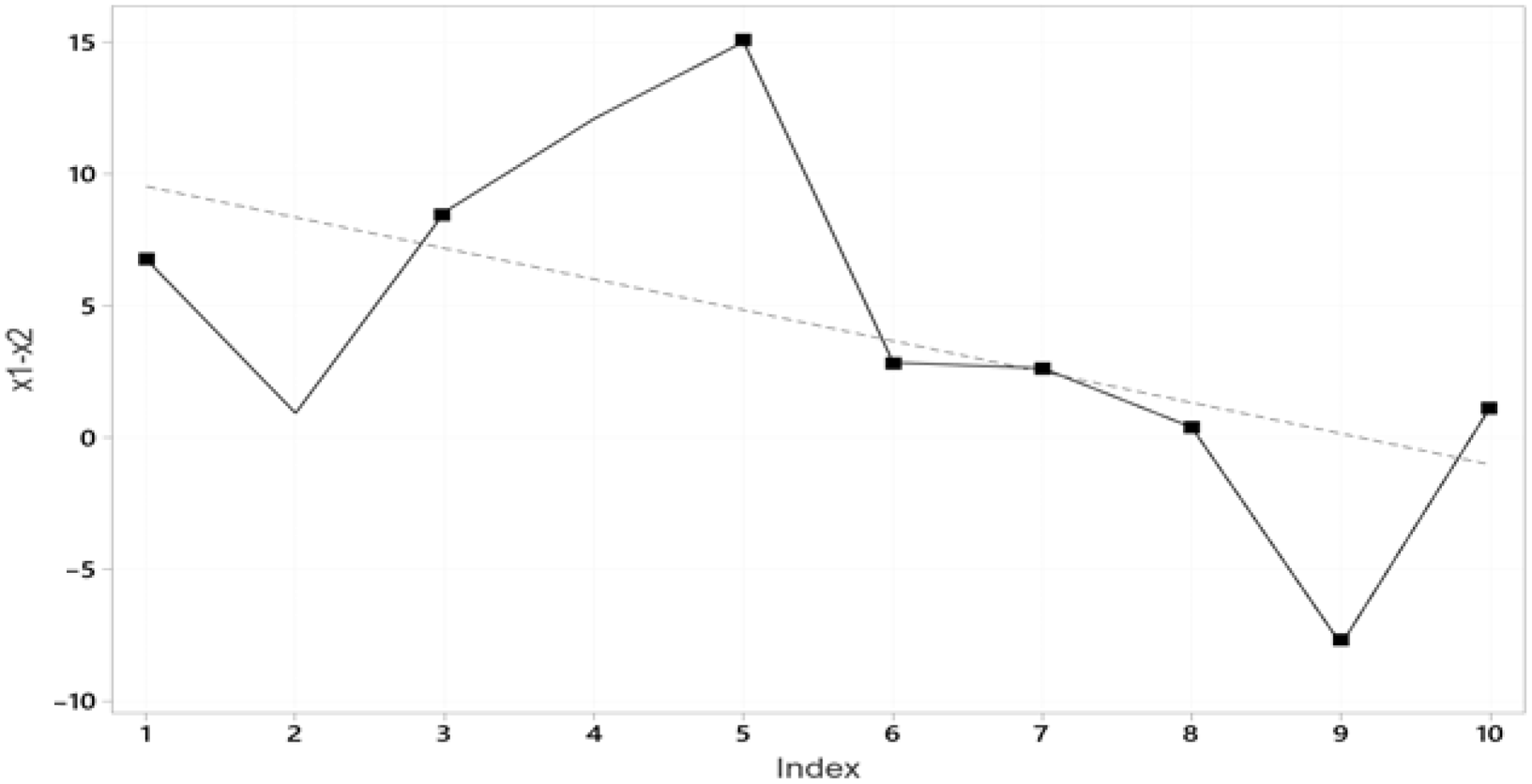
. Leaving Normality aside, a typical departure from the (ID) assumption often comes in the form of a trending mean (compare figures 2 and 3), and for the (I) assumption as irregular cycles (figure 2, from Yule Reference Yule1926) (see Spanos Reference Spanos2019, ch. 5). To detect the irregular cycles pattern in figure 1, a large enough n is needed for the cycles to recur (unfold) several times to establish a pattern; a chance regularity. For
 $n = 10,$
figure 1 would give the misleading impression of a trending mean, as opposed to
 $n \ge 40,$
where the cycles are clear.
t-plot of z t .

t-plot of y t = (x 1t – x 2t ), t = 1, 2, …, n.

Residuals from (11).

[ii] The effectiveness of inference for an estimator
 $\widehat \theta ({\bf{X}})$
is usually evaluated in terms of how well it pinpoints
 ${\theta ^ * },$
which is framed using optimal properties relating to its sampling distribution
 $f(\hat \theta ({\bf{x}});\theta ),\ {\bf{x}} \in {\mathbb R}_{\bf{X}}^{\bf{n}},$
with
 $E(\widehat \theta ({\bf{X}}))$
and
 $Var(\widehat \theta ({\bf{X}}))$
often as measure of its location and precision, respectively. The effectiveness of an N-P test or a Confidence Interval (CI) is also evaluated using their respective sampling distributions to calibrate their optimality in terms of the relevant error probabilities, type I, II, power for a test, and coverage for a CI. All these measures of effectiveness, however, presuppose [i]
 ${{\cal M}_{\bf\theta} }({\bf{x}})$
is statistically adequate so that all the relevant nominal (assumed) error probabilities (predata and postdata) approximate closely the actual ones. A crucial contributor to the ineffectiveness of inference is a “small n,” i.e., insufficient data information. Condition [ii] is needed to ensure that there is sufficient information in the particular data set
 ${{\bf{x}}_0}$
for the inference procedure to have adequate capacity to shed light on the substantive questions of interest. In particular, for an optimal N-P test
 ${T_\alpha }$
the predata error probabilities (type I and power) ensure that
 ${T_\alpha }$
has sufficient generic capacity (power) to detect discrepancies from the
 ${H_0}$
, especially the ones of substantive interest.
In conclusion, evaluating the postdata severity of untrustworthy evidence (stemming from
 $\neg $
[i], or/and
 $\neg $
[ii], where “
 $\neg $
” denotes negation) is pointless since the relevant actual error probabilities (including the p-value and severity) are likely to be different from the nominal (derived assuming
 ${{\cal M}_{\bf\theta} }({\bf{x}})$
is statistically adequate) ones.
2.3 Statistical adequacy and misspecification (M-S) testing
Establishing the statistical adequacy of
 ${{\cal M}_{\bf\theta} }({\bf{x}})$
calls for testing the validity of its probabilistic assumptions vis-a-vis data
 ${{\bf{x}}_0}$
, such as NIID in the case of (1). The most effective way to secure statistical adequacy is to separate the modeling, which includes (a) specification—the initial choice of
 ${{\cal M}_{\bf\theta} }({\bf{x}})$
, (b) M-S testing, and (c) respecification when any of its assumptions are found wanting, from the inference facet because (i) the latter presumes the statistical adequacy of
 ${{\cal M}_{\bf\theta} }({\bf{x}})$
and (ii) they pose very different questions to the data (see Spanos Reference Spanos and Rojo2006). The modeling facet aims to secure the validity of
 ${{\cal M}_{\bf\theta} }({\bf{x}})$
, presumed by the inference facet in ensuring the optimality of inference procedures with a view to secure the reliability and precision of inferential results. Treating the two as a single combined inference problem is akin to conflating the construction of a boat to given specifications (modeling) with sailing it in a competitive race (inference). The two are clearly related since the better the construction the more competitive the boat, but imagine trying to build a boat from a pile of plywood in the middle of the ocean while racing it.
Since inference presupposes the validity of
 ${{\cal M}_{\bf\theta} }({\bf{x}}),$
statistical adequacy needs to be secured before optimal inference procedures can be reliably employed. Neyman-Pearson (N-P) constitutes testing within
 ${{\cal M}_{\bf\theta} }({\bf{x}})$
aiming to narrow down
 $\Theta $
to a much smaller subset, presupposing its validity. In contrast, M-S testing poses the question whether the particular
 ${{\cal M}_{\bf\theta} }({\bf{x}})$
could have given rise to data
 ${{\bf{x}}_0}$
for any value of
 $\theta \in \Theta$
and constitutes testing outside
 ${{\cal M}_{\bf\theta} }({\bf{x}})$
since the default null
 ${{\cal M}_{\bf\theta} }({\bf{x}})$
is valid versus its negation
 $\neg {{\cal M}{\bf\theta} }({\bf{x}})\!\!: = \left[ {{\cal P}({\bf{x}}) - {{\cal M}_{\bf\theta} }({\bf{x}})} \right],$
i.e., some other statistical model in
 $\left[ {{\cal P}({\bf{x}}) - {{\cal M}_{\bf\theta} }({\bf{x}})} \right],$
where
 ${\cal P}({\bf{x}})$
is the set of all possible statistical models that could have given rise to
 ${{\bf{x}}_0}.$
The problem in practice is how to operationalize
 $\left[ {{\cal P}({\bf{x}}) - {{\cal M}_{\bf\theta} }({\bf{x}})} \right]$
to render possible comprehensive M-S testing (see Spanos Reference Spanos2018).
In addition to the above arguments, the separation of the modeling and inference facets can be formally justified in the case of statistical models whose underlying distribution belongs to the Exponential family, which includes the Normal, exponential, gamma, chi-square, beta, Bernoulli, Poisson, etc. As shown in Spanos (Reference Spanos2010), in that case
 $f({\bf{x}};{\bf\theta} ),$
in terms of which
 ${{\cal M}_{\bf\theta} }({\bf{x}})$
is specified, simplifies to:
 $$f({\bf{x}};{\bf\theta} ) = \left| J \right|\cdot f({\bf{s}},{\bf{r}};{\bf\theta} ) = \left| J \right|\cdot f({\bf{s}};{\bf\theta} )\cdot f({\bf{r}}),{\rm{ }}\forall \left( {{\bf{s}},{\bf{r}}} \right) \in {\mathbb R}_S^m \times {\mathbb R}_R^{n - m},$$
where
 $\left| J \right|$
denotes the Jacobian of the transformation
 ${\bf{X}} \to ({\bf{S(X),}}\;{\bf{R(X)}}),$
(a)
 ${\bf{R}}({\bf{X}})\!\!: = ({R_1},...,{R_{n - m}}{\bf{),}}$
is a complete sufficient statistic, (b)
 ${\bf{S(X}})\!\!: = ({S_1},...,{S_m}{\bf{)}}$
a maximal ancillary statistic, and (c)
 ${\bf{S(X)}}$
and
 $\;{\bf{R(X)}}$
are independent.
The clear separation of
 $f({\bf{s}};{\bf\theta} )\;$
and
 $f({\bf{r}})$
in (5) stemming from (c) implies that inference can be based exclusively on
 $f({\bf{s}};{\bf\theta} )$
, since the likelihood function reduces to
 $L({\bf\theta} {\bf{;}}\ {{\bf{x}}_0}) \propto f({\bf{s}};{\bf\theta} ),\;\forall {\bf\theta} \in \Theta .$
In contrast,
 $f({\bf{r}})$
can be used to validate
 ${{\cal M}_{\bf\theta} }({\bf{x}})$
using M-S testing since it is free of
 ${\bf\theta} $
, in terms of which all inferences are framed. It turns out that in the case of the simple Normal model in (1),
 ${\bf{S(X}}) = ({\overline X _n},{s^2})$
and
 ${\bf{R(X}}) = ({\widehat v_3},..,{\widehat v_n}),$
 ${\widehat v_k} = {\bf{(}}\sqrt n ({X_k} - {\overline X _n})/s),$
 $k\,{\bf{ =\, }}3,4,..,n,$
are the studentized residuals; see Spanos (Reference Spanos2018).
3. The Rochefort-Maranda example revisited
The case against the postdata severity evaluation by Rochefort-Maranda (Reference Rochefort-Maranda2020) is based on the following numerical example based on simulated data.
Example 2 Rochefort-Maranda. Consider the statistical model:
 $$\matrix{ {{{\cal M}_{\bf\theta} }({\bf{x}}){\rm{:\ }}{X_{1t}} \sim {\rm{NIID}}\,\left( {{\mu _1},{\sigma ^2}} \right),\;{X_{2t}} \sim {\rm{NIID}}\,\left( {{\mu _2},{\sigma ^2}} \right),\;t = 1,2,...,n,...,} \cr } $$
which for
 ${Y_t} = \left( {{X_{1t}} - {X_{2t}}} \right)$
becomes a special case of example 1 in (1):
 $$\matrix{ {{{\cal M}_{\bf\theta} }({\bf{y}}){\rm{:}}\ {Y_t} \sim {\rm{NIID}}\left( {\gamma ,2{\sigma ^2}} \right),\;t = 1,2,...,n,...,} \cr } $$
where
 $\gamma = \left( {{\mu _1} - {\mu _2}} \right)$
, and the hypotheses of interest are:
 $$\matrix{ {{H_0}{\rm{:}}\ \gamma \le {\gamma _0}\ {\rm{vs}}{\rm{.}}\ {H_0}{\rm{:}}\ \gamma \gt {\gamma _0},\;{\rm{for}}\ {\gamma _0} = 0.} \cr } $$
Hence, the test for (8) is a special case of the t-test in (3) with:
 $$\matrix{ {\tau ({\bf{Y}}) = [\sqrt {{n \over 2}} (\widehat \gamma - {\gamma _0})/{s_p}],\;{C_1}(\alpha ) = \{ {\bf{y}}{\rm{:}}\ \tau ({\bf{y}}) \gt {c_\alpha }\} ,\;\gamma = \left( {{\mu _1} - {\mu _2}} \right).} \cr } $$
Rochefort-Maranda (Reference Rochefort-Maranda2020) prespecified the significance level to be
 $\;\alpha = 0.05,\;{c_\alpha } = 1.833,$
and his statistical analysis is based on simulated data
 $\left\{ {({x_{1t}},{x_{2t}}),\;t = 1,2,...,n} \right\}$
for
 $n = 10$
using R (see his appendix), assigning the following values to the unknown parameters in (6),
 ${\mu _1} = 1.0,\;{\mu _2} = 1.01,\;$
 ${\sigma ^2} = 36,\gamma = 0.01.$
The resulting estimates of the parameters are:
 $$\matrix{ {\overline y = \left( {{{\overline x }_1} - {{\overline x }_2}} \right) = 2.689 - ( - 1.561) = 4.25,\;{s_p} = 4.965,} \cr } $$
yielding
 $\tau ({{\bf{y}}_0}) = {{\sqrt 5 (4.25)} \over {4.965}} = 1.914$
, with a p-value,
 $p({{\bf{y}}_0}) = 0.036$
, rejecting
 ${H_0}.$
A closer look at these numerical values raises several issues relating to the potential untrustworthiness of evidence that render the above example problematic on statistical adequacy and inference effectiveness grounds.
First, there is the issue relating to the statistical adequacy of
 ${{\cal M}_{\bf\theta} }({\bf{y}})$
in (7). Although the data come from simulation, there is always a chance that
 ${{\cal M}_{\bf\theta} }({\bf{y}})$
is misspecified for particular data
 ${{\bf{y}}_0}$
as a result of a “bad draw,” especially when
 $n = 10$
. A simple way to detect a “bad draw” is to look at the t-plot of the Rochefort-Maranda (Reference Rochefort-Maranda2020) data in figure 2, which indicates a mean-trend (decreasing) shown by the inserted trend line. To corroborate that, a simple regression of a scaled trend
 ${t_s} \in [ - 1,1]$
on
 ${y_t}$
yields:
 $$\matrix{ {{y_t} = \mathop {4.25}\limits_{(1.85)} - \mathop {5.26}\limits_{(2.90)} {t_s} + {{\widehat \varepsilon }_t},\;s = 5.861,} \cr } $$
where the standard errors, given in brackets underneath the estimates, indicate that both coefficients are statistically significant for
 $\alpha = 0.05$
. Corroborating evidence for trending data comes from comparing figures 2 and 3, the t-plot of the residuals from (11), as well as the t-plots of NIID data in figures 8–9. Although
 $n = 10$
is too small for effective misspecification testing, the above results are indicative of a departure from the ID assumption (see Spanos Reference Spanos2018).
More formally, the results in (11) indicate that
 ${{\cal M}_{\bf\theta} }({\bf{x}})$
in (6) is misspecified (ID is invalid), and the Rochefort-Maranda (Reference Rochefort-Maranda2020) estimates,
 $\overline y = 4.25$
and
 ${s_p} = 4.965,$
are based on inconsistent estimators since
 $E({Y_t}) = {\delta _0} + {\delta _1}{t_s}$
and
 $Var({Y_t}) = $
 $E{({Y_t} - {\delta _0} - {\delta _1}{t_s})^2}$
, whose values from consistent estimators are:
 $\widehat E({Y_t}) = $
 $4.25$
 $- 5.26{t_s}$
and
 $\widehat \sigma = 5.861;$
note that
 $\widehat \sigma $
is much closer to the true value
 $\sigma = 6$
than sp
. These inconsistencies will induce sizeable discrepancies between the actual and nominal error probabilities in testing and interval estimation (Spanos and McGuirk Reference Spanos and McGuirk2001), rendering his inference results untrustworthy.
Second, another way to corroborate that
 ${{\bf{y}}_0}$
in figure 2 is a “bad draw” is to evaluate the fragility of the Rochefort-Maranda (Reference Rochefort-Maranda2020) rejection result to two minor changes. The first is to increase n one observation at a time using his simulation program to see how
 $p({{\bf{y}}_0})$
changes. As shown below,
 $p({{\bf{y}}_0})$
changes drastically, reversing the rejection of
 ${H_0}$
when n increases by one data point, even though any data set
 ${{\bf{y}}_0}$
with
 $n \le 18$
is equally vulnerable to the “small n problem.”

A second potential contributor to a “bad draw” and the ensuing fragility of an inference result with a small n is a bad choice of the “seed” for the pseudorandom number generator (algorithm). The seed used by Rochefort-Maranda (Reference Rochefort-Maranda2020) for the data in figure 2 is “31,” which is an unfortunate choice due to its smallness (see Devroye Reference Devroye1986). It’s not obvious why the author did not use the seed “31” when simulating other NIID data in the same paper and instead replaced it with better choices “735653281” and “7356581”; much larger numbers. Replacing “31” with the other two seeds and simple variations on “7356581” by adding a digit, all the t-tests reverse the author’s result of rejecting
 ${H_0}$
, indicating how odd the choice of “31” is.

Third, even if one were to ignore the fact that
 ${{\cal M}_{\bf\theta} }({\bf{y}})$
in (6) is misspecified, the Rochefort-Maranda (Reference Rochefort-Maranda2020) estimation and testing results will be highly uninformative even with a “good draw” of data for
 $n = 10$
. Why? The point estimator
 $\left( {{{\overline x }_1} - {{\overline x }_2}} \right) = 4.25$
is 425 times larger than
 ${\gamma ^ * } = 0.01$
, and the one-sided 0.95 observed CI:
 $C{I_L}(\gamma ;{{\bf{y}}_0}) = [.4,\;\infty )$
excludes
 ${\gamma ^ * } = 0.01$
, rendering the point estimates hopelessly uninformative for any learning from data about
 ${\gamma ^ * }.$
The testing results are also uninformative since the power of the t-test in (9) to detect
 ${\gamma ^ * } = 0.01$
for
 $\alpha = 0.05$
is
 ${\cal P}(0.01) = 0.05034$
 $\alpha = 0.2$
 ${\cal P}(0.01) = 0.204$
 $\alpha = 0.5$
 ${\cal P}(0.01) = 0.505$
; i.e., the power for a discrepency 0.01 is slightly greater than
 $\alpha \;$
(figure 4), since the noncentrality parameter is tiny,
 ${\delta _1} = 0.0045$
.
Power curve (—true σ, - - -estimated σ) for γ > 0.

To evaluate the extent of the t-test’s ineffectiveness, one can use a predata calculation to reveal the n needed to ensure high enough power, say
 ${\cal P}(0.01) = 0.8,$
that yields:
 $$\mathcal{P}(0.01)\,\mathbf{\mathit{=}}\,\mathbb{P}([\sqrt {{n \over 2}}(\widehat{\gamma })/s_{p}]\gt-0.8834;\gamma _{1}\mathit{\,=\,}0.01)\mathit\,{=}\,0.8\rightarrow n\,\mathit{=}\, 3637900$$
There is worse, since
 $\sigma = 6$
is known one can evaluate the “true” power for
 ${\cal P}(0.01) = 0.8$
, which will increase the needed sample size to
 ${n^ * } = 5312800.$
The difference,
 ${n^ * } - n = 1674900$
, induces discrepancies between the true (
 $\sigma = 6$
—solid line) with the estimated (
 ${s_p} = 4.965$
—dashed line) power curves in figure 4 which increase with γ1.
The above unreliability and ineffectiveness associated with the Rochefort-Maranda (Reference Rochefort-Maranda2020) example renders learning from data about
 ${\gamma ^ * }$
an impossible task.
3.1 Severity curve and underpowered tests
Example 2 (continued). For
 $\tau ({{\bf{y}}_0}) = 1.914,$
reject
 ${H_0},$
the severity curve is:
 $$SEV(T_{\alpha };{\bf{y}}_{0};\gamma \mathit{\gt}\gamma _{1})\,\mathit{=}\,\mathbb{P}(\tau (\mathbf{Y})\leq \tau ({\bf{y}}_{0});\ \gamma \,\mathit{=}\,\gamma _{1}), \text{for} \text{all }\, \gamma _{1}\mathit{\geq }0\mathbf{,}$$
where the probability is attached to the relevant inferential claim
 $\gamma \gt {\gamma _1}$
, and not to
 ${\gamma _1}.$
In contrast to the power, this postdata evaluation is data-specific in the sense that it depends crucially on
 $\tau ({{\bf{y}}_0})$
. Instead of deriving the severity curve in (15) (figure 5, table 2), Rochefort-Maranda (Reference Rochefort-Maranda2020) cherry-picks a particular discrepancy
 ${\gamma _1} = 0.1,$
 $SEV(\gamma \gt 0.1) = .961$
, and misinterprets the assignment of probability
 $0.961$
meant for the inferential claim
 $\gamma \gt 0.1$
as an endorsement for
 ${\gamma _1} = 0.1$
; it is not! Also, the criticism ignores the fact that the severity curve (figure 5) reflects fully the uninformativeness and imprecision of the power curve (figure 4).
SEV curves (—true σ, - - -estimated σ) for γ > 0.

Power of t-test (9) with actual
 $\sigma = 6$
 $\mathop {\mathop {\gamma \gt 0}\limits^{\quad \quad } }\limits_{\quad \quad } $ |
0.01 | 0.1 | 0.2 | 0.5 | 1 | 2 |
|---|---|---|---|---|---|---|
 $\mathop {\mathop {{\cal P}(\gamma )}\limits_{\quad \quad } }\limits^{\quad \quad } = $ |
0.0503 | 0.0530 | 0.0562 | 0.067 | 0.0891 | 0.153 |
Severity of Reject
 ${H_0}$
:
 $\gamma = ({\mu _1} - {\mu _2}) = 0$
vs.
 ${H_1}$
:
 $\gamma \gt 0$
’ with (
 ${T_\alpha };{{\bf{y}}_0})$
 $\mathop {\mathop {\gamma \gt 0}\limits^{\quad \quad } }\limits_{\quad \quad } $ |
0.01 | 0.02 | 0.04 | 0.08 | 0.1 | 0.2 | 0.4 | 0.6 | 1.0 | 4.25 | 8.0 |
|---|---|---|---|---|---|---|---|---|---|---|---|
 $\mathop {\mathop {{\rm{Sev}}(\gamma \gt 0)}\limits_{\quad \quad } }\limits^{\quad \quad } = $ |
0.964 | 0.9636 | 0.9629 | 0.962 | 0.961 | 0.958 | 0.95 | 0.941 | 0.92 | 0.5 | 0.054 |
In addition, despite its uninformativeness, stemming from
 $n = 10,$
the severity curve gives a coherent account of evidence for all inferential claims
 $\gamma \gt {\gamma _1}$
since: (i)
 $SEV(\gamma \gt 0.01) = 0.964$
is larger than
 $0.961,$
as it should be. (ii)
 $SEV(\gamma \gt 4.25) = 0.5,$
which is clearly no endorsement of an “estimation-based effect size”
 ${\gamma _1} = 4.25$
; that would require severity 0.9 and above. (iii) The severity curve (figure 5) reflects a similar discrepancy between the true and estimated
 $\sigma \;$
curves, in the power curve (figure 4), whose insensitivity/uninformativeness is naturally reflected in the severity curve.
3.2 Untrustworthy evidence: Rochefort-Maranda example
The main conclusion about the Rochefort-Maranda (Reference Rochefort-Maranda2020) example is that the “bad draw” of simulated data (figure 2), with
 $n = 10$
, illustrates how one can generate untrustworthy evidence (stemming from inconsistent estimators of
 $\gamma $
and
 $\sigma $
and an underpowered test) and declare severity as the culprit for the ensuing dubious results and their evidential interpretation. His discussion ignores the two preconditions, [i] securing the statistical adequacy of
 ${{\cal M}_{\bf\theta} }({\bf{y}})$
, in combination with [ii] employing optimal inference procedures based on sufficiently large sample size n, to ensure the trustworthiness of evidence. Hence, the estimation and testing statistics, including
 $\tau ({{\bf{y}}_0}),$
 $p({{\bf{y}}_0})$
,
 ${\cal P}(.01)$
, and
 $SEV(\gamma \gt 0.01)$
, are both unreliable and imprecise, which is clearly reflected in the fragility of the p-value in (12).
Worse still, Rochefort-Maranda (Reference Rochefort-Maranda2020) proposes to address the low-power problem by increasing n, which will render the severity equally effective as the power! He also suggests that the use of replication can eliminate untrustworthy evidence. Replicating
 $n = 10$
many times, say
 $N = 10,000,$
will not address the inherent problem of untrustworthiness since the same preconditions, [i] statistical adequacy of
 ${{\cal M}_{\bf\theta} }({\bf{y}})$
, and [ii] effectiveness of inference procedures for a given n, for each replication, are required to secure the trustworthiness of the replication results. Implementing conditions [i]–[ii] and increasing n, however, will eliminate at the outset the problem of underpowered tests. This is also relevant for meta-analysis where the results of several individual studies are aggregated. Combining inferential results based on statistically adequate with those based on misspecified statistical models will result in untrustworthy evidence.
In concluding the discussion, it is important to emphasize the fact that even when
 ${{\cal M}_{\bf\theta} }({\bf{y}})$
is statistically adequate, detecting a tiny discrepancy
 $\left( {{\mu _1} - {\mu _2}} \right) = 0.01$
will still be a hopeless task with
 $n = 10$
. Intuitively, this amounts to attempting to use
 $n = 10$
data points to distinguish between two almost identical densities N
 $\left( {1.01,36} \right)$
and N
 $\left( {1,36} \right)$
(figure 6). Such a task seems worse than finding a needle in a haystack. Hence the huge sample size (
 ${n^ * } = 5312800$
) called for.
N(1, 36) vs. N(1.01, 36).

3.3 Trustworthy evidence: An example
To further illustrate the problems associated with the Rochefort-Maranda (Reference Rochefort-Maranda2020) example 2, consider contrasting its inference results with a better designed simulation example (figure 7), which is chosen to ensure that the inferential task is not as hopeless as that of figure 6.
N(1, 1) vs. N(1.3, 1).

Example 3 Consider the following simple Normal model:
 $$\matrix{{{{\cal M}_{\bf\theta}}({\bf{y}}){\rm{:}}}{{X_{1t}} \sim {\rm{NIID}}\left( {1.3,1} \right),\;{X_{2t}} \sim {\rm{NIID}}\left( {1.0,1} \right),\;t = 1,2,...,n,...,}\cr} $$
where
 $n = 150,$
 ${\mu _1} = 1.3,{\mu _2} = 1,{\sigma ^2} = 1,$
and discrepancy
 ${\gamma ^ * } = 0.3.$
Note that
 $n = 150$
ensures that
 ${\cal P}({\gamma ^ * } = \left( {{\mu _1} - {\mu _2}} \right) = 0.3) \ge 0.8.$
To avoid problems relating to (i) bad draws and (ii) nontypical realizations, one needs to plot the simulated data and perform a few misspecification tests to ensure the approximate validity of the NIID assumptions in (16).
Statistical adequacy. Looking at t-plots of the data in figures 8–9 one cannot detect any obvious departures; a conclusion affirmed by formal misspecification testing of NIID (see Spanos Reference Spanos2019).
Effective inference. The relevant statistics for testing the hypotheses in (8) are:
 $${\matrix{ {n = 150,\;\alpha = 0.05,\;{c_\alpha } = 1.645,\;\left( {{{\overline x }_1} - {{\overline x }_2}} \right) = \left( {1.294 - 0.9434} \right) = 0.351,\;{s_p} = 1.026.} \cr }} $$
The numerical values in (17) yield:
 $\matrix{ {\tau ({{\bf{y}}_0}) = {{\sqrt {75} (0.351)} \over {1.026}} = 2.963,\;p({{\bf{y}}_0}) = 0.002,} \cr } $
rejecting
 ${H_0}$
for any
 $\alpha \gt 0.002.$
t-plot of x 1t , t = 1, 2, …, n.

t-plot of x 2t , t = 1, 2, …, n.

In contrast to the Rochefort-Maranda (Reference Rochefort-Maranda2020) example 2:
(i) The power of the t-test, based on (17), to detect the true discrepancy
 ${\gamma ^ * } = 0.3$
is high,
 ${\cal P}({\gamma ^ * } = 0.3) = 0.812$
, in contrast to example 2 where
 ${\cal P}({\gamma ^ * } = 0.01) = 0.05034.$
It is also considerably more sensitive to discrepancies
 ${\gamma _1} \in (0,0.6)$
:
 ${\cal P}({\gamma _1} = 0.15) = 0.353,$
 ${\cal P}({\gamma _1} = 0.2) = 0.517,$
 ${\cal P}({\gamma _1} = 0.25) = 0.679, $
 $ {\cal P}({\gamma _1} = 0.3) =0.812$
,
 ${\cal P}({\gamma _1} = 0.5) = 0.994$
,
 ${\cal P}(2{\gamma ^ * }) = 1$
; see figure 10.
Power curve for example 3 in (17).

(ii) The one-sided
 $0.95$
 $C{I_L}(\gamma ;{{\bf{y}}_0}) = [.156,\infty ),$
includes
 ${\gamma ^ * } = 0.3$
, in contrast to example 2.
(iii) The severity curve (figure 11) is considerably more sensitive to small discrepancies on either side of
 ${\gamma ^ * } = 0.3$
:
 $SEV(\gamma \gt 0.15) = 0.955,\;$
 $SEV(\gamma \gt 0.2) = 0.9,$
 $SEV(\gamma \gt 0.25) = 0.802,$
 $SEV(\gamma \gt 0.3) = 0.667,$
 $SEV(\gamma \gt 0.4) = 0.339, $
 $SEV(\gamma \gt 0.5) = 0.104.$
SEV curve for γ > 0 based on (17).

Features (i)–(iii) describe what trustworthy evidence look like.
In conclusion, it is important to emphasize that the large (small) n problems create serious conundrums when testing results are to be transformed into evidence for or against
 ${H_0}$
. Worse, detaching accept/reject
 ${H_0}$
, at some
 $\alpha = 0.025,0.05,\;0.001,$
from its particular statistical context:
 $$ (i)\ {{\cal M}_{\bf\theta} }({\bf{y}}),\;(ii)\ {H_0}:\theta \in {\Theta _0}\ vs.\ {H_1}:\theta \in {\Theta _1},(iii)\ {T_\alpha }: = \{ d({\bf{Y}}),{C_1}(\alpha )\} ,(iv)\ \rm data\ {{\bf{y}}_0},$$
renders any evidential interpretation dubious. This has generated numerous misinterpretations of the p-value and contributed significantly to the misuse of frequentist testing (Spanos Reference Spanos2014), including underpowered tests. A key difference between severity and other attempts to provide an evidential interpretation of testing results is that the outputting of the warranted discrepancy
 $\gamma $
takes into account the statistical context in (18) that includes the power and n.
4. “The more power the better” for what?
4.1 Predata versus postdata error probabilities
This distinction was introduced by Hacking (Reference Hacking1965, 88), in the form of the initial (before-trial bets) versus final precision (after-trial bets) of N-P testing, calling into question the appropriateness of the predata error probabilities (type I and power) when used to evaluate evidentially the accept/reject
 ${H_0}$
results postdata. The Neyman-Pearson (Reference Neyman and Pearson1933) recasting of Fisher’s significance testing is sometimes presented as an inconsistent hybrid “burdened with conceptual confusion” (Gigerenzer Reference Gigerenzer1993, 323). There is an element of truth in this claim as it relates to the traditional recasting of the accept/reject
 ${H_0}$
rules in terms of the p-value:
[i] if
 $p({{\bf{y}}_0}) \gt \alpha ,\;$
accept
 ${H_0},$
[ii] if
 $p({{\bf{y}}_0}) \le \alpha ,\;$
reject
 ${H_0}.$
As argued in Spanos (Reference Spanos2019), however, the apparent inconsistency arises because the traditional definition of the p-value as “the probability of obtaining a result ‘equal to or more extreme’ than the one observed,”
 ${{\bf{y}}_0}$
, when
 ${H_0}$
is true, is misleadingly linked with N-P predata considerations since the clause “equal to or more extreme” is invariably interpreted with respect to
 ${H_1}$
. The link and the inconsistency disappear by adopting a postdata definition of the p-value as “the probability of all sample realizations
 ${\bf{y}}$
that accord less well with
 ${H_0}$
than
 ${{\bf{y}}_0}$
does, when
 ${H_0}$
is true”. This ensures that
 $p({{\bf{y}}_0})$
is always one-sided because the sign of
 $\tau ({{\bf{y}}_0})$
(and not
 ${H_1}$
) indicates the relevant direction of departure from
 ${H_0}$
(see Spanos Reference Spanos2013b, Reference Spanos2014).
4.2 The sample size (n) and evidence for or against
${H_0}$

The Rochefort-Maranda (Reference Rochefort-Maranda2020) slogan “the more power the better” is a sensible strategy predata, but postdata one needs to safeguard the results from the fallacies of acceptance and rejection by taking into account the generic (for any
 $\mathbf{y}\mathit{\in }\mathbb{R}_{Y}^{n}\mathbf{)}$
capacity of the particular test
 ${T_\alpha }$
, in outputting the warranted discrepancy
 $\gamma $
for data
 ${{\bf{y}}_0}$
. Intuitively, a test with high power could pick up even tiny discrepancies
 ${H_0}$
. In contrast, a test with low power could only detect sizeable discrepancies. When both find statistically significant discrepancies from
 ${H_0}$
, the less powerful test provides better evidence for the presence of a discrepancy.
Indeed, his followup claim that “the more powerful a test that rejects
 ${H_0}$
, the more the evidence against
 ${H_0}$
,” constitutes a misconception. This claim is based on misunderstanding the difference between aiming for “a large n” predata to increase the power of the test (a commendable strategy) and what the particular power implies, postdata (for a given
 ${{\bf{y}}_0}),$
in terms of evidence for or against
 ${H_0}$
.
Pratt (Reference Pratt1961, 166) pinpointed this misconception, arguing that: “the more powerful the test, the more a just significant result favors the null hypothesis.”
Example 4 To illustrate Pratt’s correct answer, consider testing the hypotheses in (2) for
 ${\mu _0} = 0.5$
in the context of (1) with
 $\sigma = 2$
and
 $\alpha = 0.025$
(
 ${c_\alpha } = 1.96$
), where:
 $$\eqalign{A - [n = 547480,\;\widehat \mu = 0.5053,\;\sqrt {Var(\widehat \mu )} = 0.0027]\ \cr{\rm and \ B} - [n = 50,\;\widehat \mu = 1.0572,\;\sqrt {Var(\widehat \mu )} = 0.28284]} $$
the two practitioners A and B with different n and
 $\widehat \mu $
find just significant results:
 $${\matrix{ {{\rm{(A)}}\;{d_1}({{\bf{x}}_0}) = \sqrt {547480} \,(.5053 - 0.5)/2 = 1.97,}\ {\rm{(B)}}\;{d_2}({{\bf{x}}_0}) = \sqrt {50} \,(1.0572 - .5)/2 = 1.97.}} $$
According to Rochefort-Maranda (Reference Rochefort-Maranda2020), test (A) provides stronger evidence against
 ${H_0}$
:
 ${\mu _0} = 0.5$
because
 ${n_1} \gt {n_2}$
. Does it? Instead of using severity, which will clearly confirm Pratt’s claim, consider their
 $0.95$
one-sided observed CIs for
 $\mu $
:
 $${\rm (A)}\ C{I_L}(\mu ;\ {{\bf{x}}_0}) = [.50001,\;\infty ),\ {\rm(B)}\ C{I_L}(\mu ;\ {{\bf{x}}_0}) = [.50283,\;\infty ).$$
The
 $C{I_L}(\mu ;{{\bf{x}}_0})$
for (A)-(
 $n = 547480)$
confirms Pratt since its lower bound is closer to
 ${H_0}$
:
 ${\mu _0} = 0.5$
than that of (B)-(
 $n = 50)$
(see also Mayo Reference Mayo2018).
5. Estimation-based versus testing-based effect sizes
The Rochefort-Maranda (Reference Rochefort-Maranda2020) example revolves around
 $\left( {{{\overline x }_1} - {{\overline x }_2}} \right) = 4.25,$
which is viewed as the “inflated effect-size” relating to an underpowered test, which yields a high Cohen’s
 $$\matrix{ {d = [({{\overline x }_1} - {{\overline x }_2})/{s_p}] = \left( {4.25/4.965} \right) = 0.856.} \cr } $$
His discussion, however, is based on two misconceptions.
Misconception: Conflating estimation-based effect sizes with testing-based effect sizes outputted by the postdata severity evaluation of testing results.
This distinction is important because the former are grounded on another misconception that the latter is devised to circumvent.
Misconception: For a particular
 ${{\cal M}_{\bf\theta} }({\bf{x}}),$
an optimal point estimator
 $\widehat \theta ({\bf{X}})$
of
 $\theta $
does not entail the inferential claim
 $\widehat \theta ({{\bf{x}}_0}) \simeq {\theta ^ * }$
for a large enough n, wbere “
 $ \simeq $
” denotes “approximately equal to.”
Example 1 (continued). For the simple Normal model in (1), the optimal estimator
 ${\widehat \mu _{ML}}({\bf{X}}) = {1 \over n}\sum\nolimits_{i = 1}^n {X_i}$
is consistent, unbiased, and fully efficient, but does not entail
 $\widehat \mu ({{\bf{x}}_0}) \simeq {\mu ^ * }$
because the estimate
 ${\widehat \mu _{ML}}({{\bf{x}}_0})$
represents just a single value of
 ${\widehat \mu _{ML}}({\bf{X}})$
. Figure 12 depicts an approximation of
 $f({\widehat \mu _{ML}}({{\bf{x}}_0});\theta ),\ {\bf{x}} \in {\rm{ }}{{\mathbb R}^{{n}}}$
with
 $n = 100,$
 $\mu = 1$
and
 ${\sigma ^2}$
 $ = 36$
using
 $N = 10,000$
replications, where
 ${\widehat \mu _{ML}}({{\bf{x}}_0})$
can be anywhere within the range
 $[ - 2.1,3.9]$
.
Approximation of
 $\overline {{X_n}} \sim N(\mu ,{{{\sigma ^2}} \over n}),\,\,n = 100,\,\,N = 10,000$
.

That explains why a point estimate is often reported as
 $\widehat \theta ({{\bf{x}}_0}) \pm 2\sqrt {Var(\widehat \theta ({\bf{X}}))} ,$
to indicate its approximate range of possible values. This is remedied by interval estimation and hypothesis testing, both of which calibrate the relevant uncertainty using error probabilities based on
 $f(\widehat \theta ({\bf{x}} );\theta ),\;{\bf{x}} \in {\mathbb R}_X^n$
of
 $\widehat \theta ({\bf{X}}).$
To shed light on what it takes to get a value of
 ${\widehat \theta _{ML}}({\bf{X}})$
that is close enough to
 ${\mu ^ * },$
consider the above simulation example to illustrate what “unbiasedness”
 $E(\widehat \theta ({\bf{X}})) = {\theta ^ * }$
means intuitively in terms of the empirical counterpart to
 $f(\widehat{\theta }({\bf x}){\bf ;}\ \theta),\ {\bf x\mathit{\in }}\mathbb{R}^{n}$
. For that one needs to use a large number N of replicas of the original data
 ${{\bf{x}}_0},$
say
 ${{\bf{x}}_1},{{\bf{x}}_2},...,{{\bf{x}}_N},$
say
 $N = 10,000$
, to estimate
 $\widehat \theta ({{\bf{x}}_i}),\;i = 1,2,...,N,$
whose histogram in figure 12 approximates
 ${\widehat f_N}(\widehat \theta ({{\bf{x}}_1},,{{\bf{x}}_2},...,{{\bf{x}}_N}){\bf{;}}\ \theta )$
, the empirical counterpart to
 $f(\widehat \theta ({\bf{x}}){\bf{;}}\ \theta ).$
The empirical mean
 ${1 \over N}\sum\nolimits_{i \,= \,1}^N \widehat \theta ({{\bf{x}}_i})$
will approximate
 ${\theta ^ * }$
closely, i.e.,
 ${1 \over N}\sum\nolimits_{i \,= \,1}^N \widehat \theta ({{\bf{x}}_i}) = 0.998 \simeq {\theta ^ * } = 1,\ $
but no single
 $\widehat \theta ({{\bf{x}}_i}),\;i = 0,1,2,...,N$
will, unless by happenstance.
Example 2 (continued). The discussions on replication revolve around effect sizes that (implicitly) invoke the unwarranted claim
 $\widehat \theta ({{\bf{y}}_0}) \simeq {\theta ^ * }.$
For instance, Cohen’s (Reference Cohen1988) d is just a single value (an estimate)
 $\widehat \theta ({{\bf{y}}_0})$
of the point estimator:
 $\widehat \theta ({\bf{Y}}) = [({\overline X _1} - {\overline X _2})/{s_p}]$
of
 $\theta = [({\mu _1} - {\mu _2})/\sigma ].$
Numerous recent papers replicate previously published results and use the point estimate as a good approximation of the “true” effect size
 ${\theta ^ * }.$
Rochefort-Maranda’s (Reference Rochefort-Maranda2020) claim: “it is now well documented that significant tests with low power display inflated effect sizes.” His poorly designed numerical example to make his case suggests that such “inflated effect sizes” are often a reflection of the untrustworthiness of the particular evidence and the unwarrantedness of the associated inferential claim.
In contrast, the postdata severity evaluation provides a testing-based effect size in the form of the discrepancy from
 ${H_0}$
warranted by
 ${{\bf{y}}_0}$
and
 ${T_\alpha }$
. As shown in table 2, the estimation-based effect size
 $\widehat \gamma = 4.25,$
reported by Rochefort-Maranda (Reference Rochefort-Maranda2020), yields
 $SEV(\gamma \gt 4.25) = 0.5,$
which does not sanction an “inflated estimation-effect size,” as claimed since 0.5 is not high enough. The key difference between the two measures is that
 $SEV(\gamma \gt 4.25)$
places the evaluation in its proper statistical context (18), as shown in (15) by using the sampling distribution of the test statistic
 $\tau ({\bf{Y}}) = (\sqrt {{n \over 2}} ({\overline X _1} - {\overline X _2})/{s_p})$
for
 $\gamma \gt 0$
to inform the outputting of the warranted discrepancy
 $\gamma $
by assigning different probabilities to
 ${\gamma _1} \gt 0,$
for each
 ${\gamma _1}$
. This avoids the unwarranted claim
 $\widehat \theta ({{\bf{y}}_0}) \simeq {\theta ^ * }$
, which is especially pernicious when
 $n = 10$
.
6. Summary and conclusions
Rochefort-Maranda’s (Reference Rochefort-Maranda2020) case against the postdata severity evaluation, built on a numerical example using a “bad draw” of simulated data with
 $n = 10$
, illustrates how one can generate untrustworthy evidence (inconsistent estimators and an underpowered test) and declare severity as the culprit for the ensuing dubious results. His discussion is based on several misconceptions about the proper implementation and interpretation of frequentist testing. They include: (a) failing to appreciate the two preconditions, [i] securing the statistical adequacy of
 ${{\cal M}_{\bf\theta} }({\bf{y}})$
, in combination with [ii] employing optimal inference procedures based on sufficiently large sample size n that ensure the trustworthiness of evidence, as well as conflating (b) abuses/misapplications of frequentist testing with foundational problems, (c) predata with postdata error probabilities and their respective roles, and (d) estimation-based with testing-based effect sizes.
How can one explain the fact that in testing the presence of a tiny (
 $\gamma = 0.01$
) discrepancy between two means the optimal t-test requires
 $n = 5312800$
to have sufficient power, say
 $0.8$
, but does detect it anyway with
 $n = 10$
and power
 $0.05$
? It could be easily explained as stemming from a “bad draw,” giving rise to unreliable and fragile inferences. As shown in (12), adding a single observation one at a time between 11 and 18 reverses the rejection of
 ${H_0}$
in all cases. Similarly, the table in (13) shows that choosing a better seed for the simulation algorithm also reverses the rejection in every case. A potential explanation of the results in (13) is a form of “simulated data-dredging” that describes the practice of simulating hundreds of replications of size n by changing the “seed” of the pseudorandom number algorithm in search of a desired result. Applying such “simulated data-dredging” arising from modifying the author’s seed “7356581” by adding a digit between 1 and 9 at different places of that number, as in the last three entries of (13), none of the results reject
 ${H_0},$
showing how rare and fragile the author’s result is with seed “31” in example 2 above.
The best case for the Rochefort-Maranda (Reference Rochefort-Maranda2020) argument is that some practitioners are likely to abuse severity by misapplying it to untrustworthy evidence, the same way they misapply the significance level, the p-value, and the power of an N-P test. This, however, is a meritless case that stems from ignoring preconditions [i]–[ii] for a proper implementation of frequentist testing, and conflating the abuse and misintepretation of its results with legitimate foundational issues. Indeed, this argument could potentially better explain the apparent nonreplication of many other published studies.