2 Numerical details

2.1 Governing equations and numerical method

The governing equations are the incompressible Navier–Stokes and continuity equations,

(2.1) $$\begin{eqnarray}\displaystyle & \displaystyle \unicode[STIX]{x1D70C}_{\unicode[STIX]{x1D711}}\left(\frac{\unicode[STIX]{x2202}u_{i}}{\unicode[STIX]{x2202}t}+\frac{\unicode[STIX]{x2202}}{\unicode[STIX]{x2202}x_{j}}u_{i}u_{j}\right)=\unicode[STIX]{x1D6F1}_{\unicode[STIX]{x1D711}}\unicode[STIX]{x1D6FF}_{1i}-\frac{\unicode[STIX]{x2202}p}{\unicode[STIX]{x2202}x_{i}}+\unicode[STIX]{x1D707}_{\unicode[STIX]{x1D711}}\frac{\unicode[STIX]{x2202}^{2}u_{i}}{\unicode[STIX]{x2202}x_{j}\unicode[STIX]{x2202}x_{j}}+f_{i}, & \displaystyle\end{eqnarray}$$

(2.2) $$\begin{eqnarray}\displaystyle & \displaystyle \frac{\unicode[STIX]{x2202}u_{i}}{\unicode[STIX]{x2202}x_{i}}-q=0, & \displaystyle\end{eqnarray}$$

where $x_{i}$ are the Cartesian coordinates $(x,y,z)$ , $u_{i}$ are the corresponding velocity components $(u,v,w)$ , $p$ is the pressure, $\unicode[STIX]{x1D70C}$ and $\unicode[STIX]{x1D707}$ are the density and viscosity of the fluid, respectively, the subscript $\unicode[STIX]{x1D711}$ indicates water or oil (or air), $\unicode[STIX]{x1D6F1}$ is the mean pressure gradient imposed on the water flow to maintain a constant mass flow rate ( $\unicode[STIX]{x1D6F1}=0$ in the shear-driven oil or air layer). The values of $f_{i}$ and $q$ are the momentum forcing and mass source to satisfy the no-slip boundary condition and mass conservation on the longitudinal groove surfaces using an immersed boundary method (Kim, Kim & Choi Reference Kim, Kim and Choi2001). Details of the determination of $f_{i}$ and $q$ are given in Kim et al. (Reference Kim, Kim and Choi2001).

To solve (2.1) and (2.2), a semi-implicit fractional-step method, adopting a third-order Runge–Kutta method for convection terms and the Crank–Nicolson method for viscous terms, is used for time integration,

(2.3) $$\begin{eqnarray}\displaystyle \frac{\hat{u} _{i}^{k}-u_{i}^{k-1}}{\unicode[STIX]{x0394}t} & = & \displaystyle \frac{2\unicode[STIX]{x1D6FC}_{k}}{\unicode[STIX]{x1D70C}_{\unicode[STIX]{x1D711}}}\left(\unicode[STIX]{x1D6F1}_{\unicode[STIX]{x1D711}}^{k-1}\unicode[STIX]{x1D6FF}_{1i}-\frac{\unicode[STIX]{x2202}p^{k-1}}{\unicode[STIX]{x2202}x_{i}}\right)+\unicode[STIX]{x1D6FC}_{k}[L_{i}(\hat{\boldsymbol{u}}^{k})+L_{i}(\boldsymbol{u}^{k-1})]\nonumber\\ \displaystyle & & \displaystyle -\,\unicode[STIX]{x1D6FD}_{k}N_{i}(\boldsymbol{u}^{k-1})-\unicode[STIX]{x1D6FE}_{k}N_{i}(\boldsymbol{u}^{k-2})+\frac{1}{\unicode[STIX]{x1D70C}_{\unicode[STIX]{x1D711}}}f_{i}^{k},\end{eqnarray}$$

(2.4) $$\begin{eqnarray}\displaystyle & \displaystyle \frac{\unicode[STIX]{x2202}^{2}\unicode[STIX]{x1D719}^{k}}{\unicode[STIX]{x2202}x_{i}\unicode[STIX]{x2202}x_{i}}=\frac{1}{2\unicode[STIX]{x1D6FC}_{k}\unicode[STIX]{x0394}t}\left(\frac{\unicode[STIX]{x2202}\hat{u} _{i}^{k}}{\unicode[STIX]{x2202}x_{i}}-q^{k}\right), & \displaystyle\end{eqnarray}$$

(2.5) $$\begin{eqnarray}\displaystyle & \displaystyle u_{i}^{k}=\hat{u} _{i}^{k}+2\unicode[STIX]{x1D6FC}_{k}\unicode[STIX]{x0394}t\left[(\unicode[STIX]{x1D6F1}_{\unicode[STIX]{x1D711}}^{k}-\unicode[STIX]{x1D6F1}_{\unicode[STIX]{x1D711}}^{k-1})\unicode[STIX]{x1D6FF}_{1i}-\frac{\unicode[STIX]{x2202}\unicode[STIX]{x1D719}^{k}}{\unicode[STIX]{x2202}x_{i}}\right], & \displaystyle\end{eqnarray}$$

(2.6) $$\begin{eqnarray}\displaystyle & \displaystyle p^{k}=p^{k-1}+\unicode[STIX]{x1D70C}_{\unicode[STIX]{x1D711}}\unicode[STIX]{x1D719}^{k}-\unicode[STIX]{x1D707}_{\unicode[STIX]{x1D711}}\unicode[STIX]{x1D6FC}_{k}\unicode[STIX]{x0394}t\frac{\unicode[STIX]{x2202}^{2}\unicode[STIX]{x1D719}^{k}}{\unicode[STIX]{x2202}x_{j}\unicode[STIX]{x2202}x_{j}}, & \displaystyle\end{eqnarray}$$

(2.7a,b ) $$\begin{eqnarray}\displaystyle L_{i}(\boldsymbol{u})=\unicode[STIX]{x1D708}_{\unicode[STIX]{x1D711}}\frac{\unicode[STIX]{x2202}^{2}u_{i}}{\unicode[STIX]{x2202}x_{j}\unicode[STIX]{x2202}x_{j}},\quad N_{i}(\boldsymbol{u})=\frac{\unicode[STIX]{x2202}}{\unicode[STIX]{x2202}x_{j}}u_{i}u_{j}, & & \displaystyle\end{eqnarray}$$

where $\hat{u} _{i}$ are the intermediate velocity components, $\unicode[STIX]{x1D719}$ is the pseudo-pressure, $\unicode[STIX]{x1D708}_{\unicode[STIX]{x1D711}}$ is the kinematic viscosity of water or oil (or air), the subscript $k(=1,2,3)$ is the sub-step index during one time step, $\unicode[STIX]{x0394}t$ is the size of the computational time step and $\unicode[STIX]{x1D6FC}_{1}=4/15$ , $\unicode[STIX]{x1D6FC}_{2}=1/15$ , $\unicode[STIX]{x1D6FC}_{3}=1/6$ , $\unicode[STIX]{x1D6FD}_{1}=8/15$ , $\unicode[STIX]{x1D6FD}_{2}=5/12$ , $\unicode[STIX]{x1D6FD}_{3}=3/4$ , $\unicode[STIX]{x1D6FE}_{1}=0$ , $\unicode[STIX]{x1D6FE}_{2}=-17/60$ and $\unicode[STIX]{x1D6FE}_{3}=-5/12$ . Details of how to obtain $\unicode[STIX]{x1D6F1}_{\unicode[STIX]{x1D711}}^{k}$ in (2.5) are described in You, Choi & Yoo (Reference You, Choi and Yoo2000). The present numerical simulation is based on a finite volume method on a staggered grid system, and thus the velocity components are located at the cell faces, and the pressure is located at the cell centre. All spatial derivatives are discretized with the second-order central difference scheme. The maximum Courant–Friedrichs–Lewy (CFL) number varies from 0.7 to 1.4, depending on the oil used. Air-lubricated cases require smaller maximum CFL numbers than oil-lubricated ones, due to large differences in material properties across the interface.

Figure 1.

Schematic diagrams of the computational domain: (a) turbulent channel flow with micro-grooved structures; (b) cross-flow plane. Micro-grooved structures are placed only on the lower wall. Here, $H$ is the channel half-height, $D$ and $L_{g}$ are the depth and width of micro-grooves, respectively, and $L_{p}$ is the pitch length.

Figure 1 shows the computational domain and the coordinate system used in the present study. The upper wall is a flat plate, but the lower wall has micro-size longitudinal grooves. The size of longitudinal grooves is determined with reference to the experiments of Woolford et al. (Reference Woolford, Prince, Maynes and Webb2009) and Rosenberg et al. (Reference Rosenberg, Van Buren, Fu and Smits2016) in which the pitch length $L_{p}$ is of the order of one in wall units. We summarize the cases of micro-grooves considered and numbers of grid points used for simulations in table 1, where $L_{p_{o}}^{+}=L_{p}u_{\unicode[STIX]{x1D70F}_{o}}/\unicode[STIX]{x1D708}_{w}$ , $L_{g_{o}}^{+}=L_{g}u_{\unicode[STIX]{x1D70F}_{o}}/\unicode[STIX]{x1D708}_{w}$ , $D_{o}^{+}=Du_{\unicode[STIX]{x1D70F}_{o}}/\unicode[STIX]{x1D708}_{w}$ and $u_{\unicode[STIX]{x1D70F}_{o}}(=\sqrt{\unicode[STIX]{x1D70F}_{w_{o}}/\unicode[STIX]{x1D70C}_{w}})$ and $\unicode[STIX]{x1D70F}_{w_{o}}$ are the wall-shear velocity and stress in the absence of micro-grooved structures, respectively. Here, the lubricant fraction is fixed at $\unicode[STIX]{x1D6F7}=L_{g}/L_{p}=0.8$ ; it is known that more drag reduction is achieved with larger $\unicode[STIX]{x1D6F7}$ (Park et al. Reference Park, Park and Kim2013, Reference Park, Sun and Kim2014), but the interface becomes less stable at the same time (Cartagena et al. Reference Cartagena, Arenas, Bernardini and Leonardi2018), and $\unicode[STIX]{x1D6F7}=0.8$ is the one used in Woolford et al. (Reference Woolford, Prince, Maynes and Webb2009). The size of the computational domain is $L_{x}=3H,L_{y}=2H+D,L_{z}=0.84H$ , where $H$ is the channel half-height. The spanwise domain size is set to be slightly bigger than that of the minimal channel (Jiménez & Moin Reference Jiménez and Moin1991) because low-order turbulence statistics near the wall are well predicted with minimal channel unit, and a large number of grid points is required in the $z$ -direction due to micro-size grooves (see table 1). The periodic boundary condition is imposed in the $x$ and $z$ -directions. No-slip boundary condition is imposed on the upper wall and is satisfied on the longitudinal groove surfaces using an immersed boundary method (Kim et al. Reference Kim, Kim and Choi2001).

Table 1.

Geometric parameters of grooves and number of grid points used.

We assume that the oil–water and air–water interfaces are flat (Jung et al. Reference Jung, Choi and Kim2016). As discussed in § 1, this assumption is valid for the present study because the groove geometry under consideration is micro-sized and the corresponding Weber number using wall variables is of the order of $10^{-3}$ , $We^{+}=\unicode[STIX]{x1D70C}_{w}u_{\unicode[STIX]{x1D70F}}^{2}\unicode[STIX]{x1D6FF}_{v}/\unicode[STIX]{x1D70E}=\unicode[STIX]{x1D70C}_{w}u_{\unicode[STIX]{x1D70F}}\unicode[STIX]{x1D708}_{w}/\unicode[STIX]{x1D70E}=O(10^{-3})$ (Seo et al. Reference Seo, García-Mayoral and Mani2015, Reference Seo, García-Mayoral and Mani2018, see below), where $u_{\unicode[STIX]{x1D70F}}$ is the friction velocity with the interface, $\unicode[STIX]{x1D6FF}_{\unicode[STIX]{x1D708}}$ is the viscous unit length ( $\unicode[STIX]{x1D6FF}_{v}=\unicode[STIX]{x1D708}_{w}/u_{\unicode[STIX]{x1D70F}}$ ) and $\unicode[STIX]{x1D70E}$ is the surface-tension coefficient of water. The wall-parallel velocity components and shear stresses are continuous across the interface: i.e.

(2.8a,b ) $$\begin{eqnarray}u_{w,s}=u_{l,s}=u_{s},\quad w_{w,s}=w_{l,s}=w_{s},\end{eqnarray}$$

(2.9a,b ) $$\begin{eqnarray}\unicode[STIX]{x1D707}_{w}\left.\frac{\unicode[STIX]{x2202}u_{w}}{\unicode[STIX]{x2202}y}\right|_{s}=\unicode[STIX]{x1D707}_{l}\left.\frac{\unicode[STIX]{x2202}u_{l}}{\unicode[STIX]{x2202}y}\right|_{s},\quad \unicode[STIX]{x1D707}_{w}\left.\frac{\unicode[STIX]{x2202}w_{w}}{\unicode[STIX]{x2202}y}\right|_{s}=\unicode[STIX]{x1D707}_{l}\left.\frac{\unicode[STIX]{x2202}w_{l}}{\unicode[STIX]{x2202}y}\right|_{s}.\end{eqnarray}$$

Here, the subscripts $w$ , $l$ and $s$ stand for water, lubricant (oil or air) and the interface, respectively. The wall-normal velocity at the interface is zero, satisfying the impermeability condition

(2.10) $$\begin{eqnarray}v_{w,s}=v_{l,s}=v_{s}=0.\end{eqnarray}$$

The slip velocity at the interface, ( $u_{s}$ , $w_{s}$ ), is obtained by taking one-side finite difference on (2.9) for each fluid, i.e.

(2.11a,b ) $$\begin{eqnarray}\unicode[STIX]{x1D707}_{w}\frac{u_{upper}-u_{s}}{y_{upper}-y_{s}}=\unicode[STIX]{x1D707}_{l}\frac{u_{s}-u_{lower}}{y_{s}-y_{lower}},\quad \unicode[STIX]{x1D707}_{w}\frac{w_{upper}-w_{s}}{y_{upper}-y_{s}}=\unicode[STIX]{x1D707}_{l}\frac{w_{s}-w_{lower}}{y_{s}-y_{lower}},\end{eqnarray}$$

where $y_{s}(=0)$ is the $y$ location of the interface, and $y_{upper}$ and $y_{lower}$ are the cell centre locations right above and below $y_{s}$ , respectively, and $u_{upper}$ and $w_{upper}$ , and $u_{lower}$ and $w_{lower}$ are the corresponding slip velocity components. The boundary condition of the pseudo-pressure at the interface (for solving (2.4)) is given as

(2.12) $$\begin{eqnarray}\left.\frac{\unicode[STIX]{x2202}\unicode[STIX]{x1D719}_{w}}{\unicode[STIX]{x2202}y}\right|_{s}=\left.\frac{\unicode[STIX]{x2202}\unicode[STIX]{x1D719}_{l}}{\unicode[STIX]{x2202}y}\right|_{s}=0.\end{eqnarray}$$

Equation (2.3) is solved using an alternating directional implicit scheme with the interface boundary conditions (2.8)–(2.10). The Poisson equation (2.4) is Fourier transformed in the $x$ - and $z$ -directions due to the periodic boundary conditions applied (this is possible even inside the groove because we use an immersed boundary method), and the resulting tridiagonal system of equations is separately solved for two domains (below and above the interface, respectively) with the boundary condition (2.12).

The bulk Reynolds number is $Re=2\unicode[STIX]{x1D70C}_{w}u_{b}H/\unicode[STIX]{x1D707}_{w}=5600$ corresponding to $Re_{\unicode[STIX]{x1D70F}_{o}}=\unicode[STIX]{x1D70C}_{w}u_{\unicode[STIX]{x1D70F}_{o}}H/\unicode[STIX]{x1D707}_{w}\approx 180$ , where $u_{b}$ is the bulk velocity. The mass flow rate of water is maintained to be constant by imposing the mean pressure gradient $\unicode[STIX]{x1D6F1}$ , where $\unicode[STIX]{x1D6F1}$ is determined by obtaining the mean and fluctuating pseudo-pressure gradients separately at each time step (You et al. Reference You, Choi and Yoo2000).

Table 2.

Lubricants and their viscosities and densities normalized by those of water, and the percentages of drag reduction $(DR)$ for the case of $L_{g_{o}}^{+}=3$ ( $L_{p_{o}}^{+}=3.78$ ) and $D_{o}^{+}=3.6$ .

2.2 Lubricants and air

For LIS, various oils can be utilized as long as they are immiscible with the working fluid (water) and maintain a flat interface. Considered lubricants are listed in table 2, together with their viscosities and densities. FC-70 is an oil used in Wong et al. (Reference Wong, Kang, Tang, Smythe, Hatton, Grinthal and Aizenberg2011) with which the SLIPS was first introduced, whereas FC-3283 and heptane are oils used in Rosenberg et al. (Reference Rosenberg, Van Buren, Fu and Smits2016), which reported drag reductions with LISs for turbulent Taylor–Couette flow. The Weber numbers for SHS and LIS (heptane) are $We^{+}=\unicode[STIX]{x1D70C}_{w}u_{\unicode[STIX]{x1D70F}_{o}}\unicode[STIX]{x1D708}_{w}/\unicode[STIX]{x1D70E}=1.29\times 10^{-3}$ and $1.89\times 10^{-3}$ , respectively, for the case of $Re_{\unicode[STIX]{x1D70F}_{o}}\approx 180$ and $L_{p_{o}}^{+}=3.78$ ( $L_{p}=0.021H$ ; $L_{p}=40~\unicode[STIX]{x03BC}\text{m}$ ) (Woolford et al. Reference Woolford, Prince, Maynes and Webb2009). Another Weber number suggested by Seo et al. (Reference Seo, García-Mayoral and Mani2018) is $We_{L}=\unicode[STIX]{x1D70C}_{w}u_{\unicode[STIX]{x1D70F}_{o}}^{2}L_{p}/\unicode[STIX]{x1D70E}=We^{+}L_{p}^{+}$ . With $L_{p_{o}}^{+}=3.78{-}15.12$ , $We_{L}=(4.91{-}19.66)\times 10^{-3}$ for SHS and $(7.14{-}28.58)\times 10^{-3}$ for LIS (heptane), respectively. Since these Weber numbers are small, the interface can be assumed to be flat.

Table 3.

Effects of the computational domain size and grid resolution on the drag reduction ( $DR$ ; equation (3.2)) and mean slip velocity ( $\bar{u}_{s}^{tot}$ ; see below for the definition) for LIS (heptane) and SHS (air) of $L_{g_{o}}^{+}=12$ and $D_{o}^{+}=14.4$ .

The amounts of drag reduction ( $DR$ whose definition is given in § 3) with LISs from preliminary DNSs are shown in table 2 for the case of $L_{g_{o}}^{+}=3$ ( $L_{p_{o}}^{+}=3.78$ ) and $D_{o}^{+}=3.6$ ( $D=0.02H$ ). In table 2, we add two more cases of ‘water lubricant’. The case of water (rough) is to purely represent the effect of the groove geometry just like flow over riblets (Walsh Reference Walsh1983; Choi, Moin & Kim Reference Choi, Moin and Kim1993; Bechert et al. Reference Bechert, Brus, Hage, Van der Hoeven and Hoppe1997): i.e. the grooves are wet by the overlying water flow and act like a rough surface. The computational domain size in the $y$ -direction is modified such that the bottom of micro-groove structures is at $y=-0.004H$ , then the whole cross-sectional area of water flow in the presence of micro-groove structures is the same as that of flat-plate channel flow $(2H\times L_{z})$ . The case of water (interface) is to replace oil with water but maintaining the flat interface: i.e. the lubricating water layer is shear driven, whereas the working fluid (water) is pressure driven, as in figure 1. These two cases of water (rough) and water (interface) do not show significant changes in the drag due to the small size of the grooves. On the other hand, the case of heptane shows a meaningful amount of drag reduction, comparable to that of SHS. The amounts of drag variation by FC-70 and FC-3283 are much smaller than that by heptane. Therefore, we choose heptane (LIS) and air (SHS) as the lubricating materials hereinafter.

3 Drag and slip characteristics

Given a fixed mass flow rate, the mean pressure gradient in the channel varies at each time step, balanced by the skin frictions on the upper flat surface and the lower longitudinal groove surface. Since the lubricant layer is shear driven by the water flow, the sum of skin frictions on the side and bottom surfaces of the groove structure is the same as the skin friction on the interface. Thus, the drags on the upper flat and lower groove surfaces are calculated as

(3.1) $$\begin{eqnarray}\left.\begin{array}{@{}c@{}}\displaystyle D_{upper\;wall}=\frac{1}{T}\int _{0}^{T}\int _{0}^{L_{x}}\int _{0}^{L_{z}}\unicode[STIX]{x1D707}_{w}\frac{\unicode[STIX]{x2202}u}{\unicode[STIX]{x2202}y}(x,y=2H,z,t)\,\text{d}z\,\text{d}x\,\text{d}t=L_{x}L_{z}\unicode[STIX]{x1D707}_{w}\left.\frac{\unicode[STIX]{x2202}\bar{u}^{tot}}{\unicode[STIX]{x2202}y}\right|_{upper\;wall},\\ \displaystyle D_{groove}=\frac{1}{T}\int _{0}^{T}\int _{0}^{L_{x}}\int _{0}^{L_{z}}\unicode[STIX]{x1D707}_{w}\frac{\unicode[STIX]{x2202}u}{\unicode[STIX]{x2202}y}(x,y=0,z,t)\,\text{d}z\,\text{d}x\,\text{d}t=L_{x}L_{z}\unicode[STIX]{x1D707}_{w}\left.\frac{\unicode[STIX]{x2202}\bar{u}^{tot}}{\unicode[STIX]{x2202}y}\right|_{s},\end{array}\right\}\end{eqnarray}$$

respectively. Here, the superscript ‘tot’ denotes the averaging over time and space ( $x$ and $z$ ). The drag reduction is calculated as

(3.2) $$\begin{eqnarray}DR(\%)=\frac{D_{upper\;wall}-D_{groove}}{D_{upper\;wall}}\times 100.\end{eqnarray}$$

This definition relies on the observation that turbulent flow near one side of the channel does not affect the skin friction on the other side of the channel (Jiménez & Moin Reference Jiménez and Moin1991); the correlation coefficients between the shear rates at the two walls are small, $|corr|\leqslant 0.2$ , for all the cases considered. The wall-shear rates are integrated over more than $800H/u_{b}$ , and the amounts of drag reduction are listed in table 4 for the heptane- and air-lubricated cases. The drag reduction increases with increasing groove width ( $L_{g_{o}}^{+}$ ) for all the groove depths ( $D_{o}^{+}$ ) considered. On the other hand, given $L_{g_{o}}^{+}$ , the amount of drag reduction is more or less saturated even with increasing $D_{o}^{+}$ (non-monotonic behaviours of the drag reduction with the groove depth in table 4 should be regarded as a result of numerical uncertainty). Although the air layer produces larger drag reductions for the same groove sizes than the heptane layer, the amount of drag reduction by the heptane layer is still not small. Note also that a similar drag reduction is achieved when the groove width of the heptane layer is twice that of the air layer. Considering that the interface of the heptane layer is more stable under the turbulent pressure fluctuations than that of the air layer, the LIS can be an alternative to the SHS as a device for drag reduction.

Figure 2.

Spanwise variations of the friction coefficient $(\bar{c}_{f})$ on the interface and ridge: (a) heptane; (b) air. A horizontal line in (a,b) denotes the skin friction coefficient $(c_{f_{o}}=0.0083)$ of flat-plate turbulent channel flow at $Re_{\unicode[STIX]{x1D70F}_{o}}=180$ .

Table 4.

Drag reductions for the cases of heptane (LIS) and air (SHS).

Table 5.

Skin friction coefficients on the ridge and interface, and total skin friction coefficients for LIS and SHS ( $L_{g_{o}}^{+}=6,D_{o}^{+}=7.2$ , and $\unicode[STIX]{x1D6F7}=0.8$ ), and those with the shear-free condition $(L_{g_{o}}^{+}=6,\unicode[STIX]{x1D6F7}=0.8)$ , respectively. Here, $\bar{c}_{f\,ridge}$ and $\bar{c}_{f\,interface}$ denote the mean skin friction coefficients on the ridge and interface, and $\bar{c}_{f}^{tot}=(1-\unicode[STIX]{x1D6F7})\bar{c}_{f\,ridge}+\unicode[STIX]{x1D6F7}\bar{c}_{f\,interface}$ .

The spanwise variations of the time- and streamwise-averaged friction coefficient on the interface and ridge, $\bar{c}_{f}(z)$ , are shown in figures 2(a) and 2(b) for the cases of heptane and air, respectively, where $c_{f}=\unicode[STIX]{x1D70F}_{s}/(0.5\unicode[STIX]{x1D70C}_{w}u_{b}^{2})$ , $\unicode[STIX]{x1D70F}_{s}$ is the instantaneous shear stress, and the overbar denotes the averaging over the streamwise direction and time. The friction coefficients are lower on the heptane–water and air–water interfaces than that of flat plate channel flow, but are much higher on the ridge, especially near the corners ( $z/L_{g}=1$ and 1.25). Since the viscosity of air $(\unicode[STIX]{x1D707}_{R}=\unicode[STIX]{x1D707}_{w}/\unicode[STIX]{x1D707}_{a}=55.56)$ is much smaller than that of heptane $(\unicode[STIX]{x1D707}_{R}=\unicode[STIX]{x1D707}_{w}/\unicode[STIX]{x1D707}_{l}=2.7)$ , the friction coefficient on the air–water interface is smaller (almost zero except near the corners) than that on the heptane–water interface, but the one on the ridge is higher because of large slip velocity on the air–water interface (see below). The friction coefficient on the interface is nearly insensitive to the size of the groove (both $L_{g}$ and $D$ ). On the other hand, the friction on the ridge is insensitive to $D$ but depends on $L_{g}$ . With increasing $L_{g}$ , it decreases at the centre region but increases near the corner. As shown in this figure, higher drag reduction by the air layer than by the heptane layer is attributed to nearly zero shear stress at the interface, showing the validity of applying the shear-free boundary condition at the interface without solving the air layer, as demonstrated by previous studies (Martell et al. Reference Martell, Perot and Rothstein2009, Reference Martell, Rothstein and Perot2010; Park et al. Reference Park, Park and Kim2013; Jelly et al. Reference Jelly, Jung and Zaki2014; Türk et al. Reference Türk, Daschiel, Stroh, Hasegawa and Frohnapfel2014; Lee et al. Reference Lee, Jelly and Zaki2015; Rastegari & Akhavan Reference Rastegari and Akhavan2015; Seo et al. Reference Seo, García-Mayoral and Mani2015; Seo & Mani Reference Seo and Mani2016; Rastegari & Akhavan Reference Rastegari and Akhavan2018). We perform an additional simulation with the shear-free boundary condition at the interface for the case of $L_{g_{o}}^{+}=6$ and $\unicode[STIX]{x1D6F7}=0.8$ , and the results are given in table 5 together with those from LIS and SHS. When the shear-free boundary condition is applied at the interface, the predicted $\bar{c}_{f}^{tot}$ results in only 4 % error for SHS (air), but in much larger error (approximately 10 %) for LIS (heptane) due to non-negligible shear stress at the interface.

Figure 3 shows the spanwise variations of the time- and streamwise-averaged slip velocity on the heptane–water and air–water interfaces. Each slip velocity has a profile similar to $\bar{u}_{s}(z^{\ast })/\bar{u}_{s}(z^{\ast }=0.5)=2\sqrt{z^{\ast }(1-z^{\ast })}(z^{\ast }=z/L_{g})$ and is maximum at the centre of the interface (this elliptic velocity profile is analytically obtained for laminar flow if the shear rate at the interface is assumed to be constant along the spanwise direction (Schönecker et al. Reference Schönecker, Baier and Hardt2014)). The slip velocity increases with $L_{g}$ , reaching up to approximately $4u_{\unicode[STIX]{x1D70F}_{o}}$ and $6u_{\unicode[STIX]{x1D70F}_{o}}$ for the cases of heptane and air, respectively, but it is nearly insensitive to $D$ (except for the heptane with $L_{g_{o}}^{+}=12$ and $D_{o}^{+}=3.6$ ). The variation of the mean friction coefficient, $\bar{c}_{f}^{tot}$ , which is the average of $\bar{c}_{f}$ (figure 2) over the whole spanwise direction, with the slip velocity averaged over the interface and ridge, $\bar{u}_{s}^{tot}=\int _{0}^{L_{p}}\bar{u}_{s}(z)\,\text{d}z/L_{p}$ , is shown in figure 4. The $\bar{c}_{f}^{tot}$ almost linearly decreases with $\bar{u}_{s}^{tot}$ . This trend is consistent with the linear relation, $\bar{c}_{f}^{tot}/c_{f_{o}}=1-(\bar{u}_{s}^{tot}/u_{b})$ , suggested by Rastegari & Akhavan (Reference Rastegari and Akhavan2015), where $c_{f_{o}}$ is the friction coefficient of flat-plate turbulent channel flow. Figure 5 shows the root-mean-square (r.m.s.) streamwise and spanwise slip velocity fluctuations at the interface. With increasing $L_{g}$ , both $u_{s,rms}$ and $w_{s,rms}$ increase, and reach up to approximately $u_{\unicode[STIX]{x1D70F}_{o}}$ and $0.2u_{\unicode[STIX]{x1D70F}_{o}}$ for heptane, and $1.45u_{\unicode[STIX]{x1D70F}_{o}}$ and $0.3u_{\unicode[STIX]{x1D70F}_{o}}$ for air, respectively. Although the r.m.s. slip velocity fluctuations show some collapse for the same $L_{g_{o}}^{+}$ , more deviations occur at larger $L_{g_{o}}^{+}$ . Note also that the profiles of $u_{s,rms}$ and $w_{s,rms}$ follow the ellipses for smaller $L_{g_{o}}^{+}$ .

Figure 3.

Slip velocity on the interface: (a) heptane; (b) air. Lines and lines with symbols are the same as those in figure 2. Red lines are the ellipses of $\bar{u}_{s}(z^{\ast })/\bar{u}_{s}(z^{\ast }=0.5)=2\sqrt{z^{\ast }(1-z^{\ast })}$ , where $z^{\ast }=z/L_{g}$ .

Figure 4.

Mean friction coefficient versus mean slip velocity averaged over the interface and ridge. Solid line corresponds to the linear relation $\bar{c}_{f}^{tot}/c_{f_{o}}=1-(\bar{u}_{s}^{tot}/u_{b})$ from Rastegari & Akhavan (Reference Rastegari and Akhavan2015). The friction coefficient of flat-plate turbulent channel flow is $c_{f_{o}}=0.0083$ at $Re_{\unicode[STIX]{x1D70F}_{o}}=180$ .

Figure 5.

Root-mean-square (r.m.s.) slip velocity fluctuations normalized by the friction velocity $u_{\unicode[STIX]{x1D70F}_{o}}$ : (a) heptane; (b) air. Lines and lines with symbols are the same as in figure 2. Red lines are the ellipses of $u_{is,rms}(z^{\ast })/u_{is,rms}(z^{\ast }=0.5)=2\sqrt{z^{\ast }(1-z^{\ast })}(z^{\ast }=z/L_{g})$ .

Figure 6.

Normalized slip lengths: (a) slip length normalized by the groove depth and viscosity ratio; (b) slip length normalized as in (3.6) versus $z/L_{g}$ ; (c) mean slip length (3.6). In (a,b), the lines and lines with symbols are the same as in figure 2, where red and black colours denote the cases of heptane and air, respectively. In (c), the symbols are the same as those in figure 4, together with the cases of $L_{g_{o}}^{+}=3.8$ ( $\unicode[STIX]{x1D6F7}=0.5$ ) and $D_{o}^{+}=3.6$ (○, red and ○, black), and $L_{g_{o}}^{+}=1.9$ ( $\unicode[STIX]{x1D6F7}=0.5$ ) and $D_{o}^{+}=3.6$ (♢, red and ♢, black). Inset in (b) shows the slip length near the groove centre.

Since the slip velocity and velocity gradient vary over the interface, the slip length is also a function of the interface location as follows:

(3.3) $$\begin{eqnarray}\bar{b}_{x}(z)=\frac{\bar{u}_{s}(z)}{\unicode[STIX]{x2202}\bar{u}(z)/\unicode[STIX]{x2202}y|_{s}}.\end{eqnarray}$$

Figure 6 shows the slip lengths in different normalizations over the interface and the mean slip length for the cases of heptane and air. The slip length normalized by the groove depth and viscosity ratio $\unicode[STIX]{x1D707}_{R}(=\unicode[STIX]{x1D707}_{w}/\unicode[STIX]{x1D707}_{l})$ is only a function of $L_{g}/D$ irrespective of the lubricants, and they increase with increasing $L_{g}/D$ (figure 6 a). According to Jung et al. (Reference Jung, Choi and Kim2016) who considered the air–water interface in the absence of the ridges (i.e. an idealized SHS) for turbulent channel flow, the mean slip length divided by the air layer thickness ( $D$ ) is equal to the viscosity ratio $\unicode[STIX]{x1D707}_{R}$ , i.e.

(3.4) $$\begin{eqnarray}\bar{b}_{x}^{\ast }=\frac{\bar{b}_{x}}{\unicode[STIX]{x1D707}_{R}D}=1\quad (\text{for an idealized SHS}),\end{eqnarray}$$

because of the linear velocity profile within the air layer. In the present micro-groove configuration, however, the flow is affected by the no-slip condition on the ridge of the groove structure, and thus the resulting slip length is less than one, i.e.  $\bar{b}_{x}<\unicode[STIX]{x1D707}_{R}D$ (figure 6 a), and is a function of $L_{g}/D$ . When the groove is sufficiently wide as compared to its depth ( $L_{g}/D\gg 1$ ), the normalized slip length should approach one (for $L_{g}/D=3.36$ , $\bar{b}_{x}/\unicode[STIX]{x1D707}_{R}D\approx 0.9$ at the groove centre).

Considering the shear-driven Stokes flow inside the longitudinal groove, Maynes et al. (Reference Maynes, Jeffs, Woolford and Webb2007) provided the velocity distribution inside the groove and the velocity gradient at the interface using the sine series expansion. Since the component corresponding to the largest wavelength is dominant, the slip length averaged over the interface can be approximated as (using the continuity of the shear stress at the interface)

(3.5) $$\begin{eqnarray}\bar{b}_{x}^{s}=\frac{\displaystyle \int _{0}^{L_{g}}\bar{u}_{s}\,\text{d}z}{\displaystyle \int _{0}^{L_{g}}\left.\unicode[STIX]{x2202}\bar{u}/\unicode[STIX]{x2202}y\right|_{s}\,\text{d}z}=\unicode[STIX]{x1D707}_{R}\frac{\displaystyle \int _{0}^{L_{g}}u_{l}|_{s}\,\text{d}z}{\displaystyle \int _{0}^{L_{g}}\unicode[STIX]{x2202}u_{l}/\unicode[STIX]{x2202}y|_{s}\,\text{d}z}\sim \frac{1}{\unicode[STIX]{x03C0}}\unicode[STIX]{x1D707}_{R}L_{g}\tanh \frac{\unicode[STIX]{x03C0}D}{L_{g}}.\end{eqnarray}$$

Accordingly, the non-dimensional slip length from the Stokes flow approximation becomes

(3.6) $$\begin{eqnarray}\bar{b}_{x}^{\ast \ast }=\frac{\bar{b}_{x}^{s}}{\unicode[STIX]{x1D707}_{R}L_{g}\tanh (\unicode[STIX]{x03C0}D/L_{g})}\sim \frac{1}{\unicode[STIX]{x03C0}}.\end{eqnarray}$$

This result is very similar to that of Ybert et al. (Reference Ybert, Barentin, Cottin-Bizonne, Joseph and Bocquet2007), $\bar{b}_{x}=(1/q)\unicode[STIX]{x1D707}_{R}L_{g}\tanh (qD/L_{g})$ ( $q$ is a function of $\unicode[STIX]{x1D6F7}$ ), which was obtained for a square array of dilute pillars based on the Stokes flow solution for the periodic arrays of spheres by Sangani & Acrivos (Reference Sangani and Acrivos1982). Figure 6(b) shows the variations of the slip length, normalized as in (3.6), over the interface for all cases of heptane and air considered. The data scatter observed in figure 6(a) is much reduced by introducing a new normalization, (3.6). The normalized slip length at the groove centre region approaches $1/\unicode[STIX]{x03C0}$ , as the groove becomes shallow for same $L_{g}$ (i.e. increasing $L_{g}/D$ ). Figure 6(c) shows the mean slip lengths averaged over the interface as a function of $L_{g}/D$ . As shown, all the data fall on a line whose slope is 0.28, i.e.

(3.7) $$\begin{eqnarray}\bar{b}_{x}^{s}=0.28\unicode[STIX]{x1D707}_{R}L_{g}\tanh \frac{\unicode[STIX]{x03C0}D}{L_{g}}.\end{eqnarray}$$

Note that (3.7) returns to $\bar{b}_{x}^{s}/\unicode[STIX]{x1D707}_{R}D\sim 0.28\unicode[STIX]{x03C0}$ for $L_{g}\gg D$ and $\bar{b}_{x}^{s}/\unicode[STIX]{x1D707}_{R}L_{g}\sim 0.28$ for $L_{g}\ll D$ . The proportional constant, theoretically obtained, in (3.5) is $1/\unicode[STIX]{x03C0}(=0.3183)$ , and thus the difference between (3.5) and (3.7) is only 12 %, indicating that the Stokes flow approximation inside the groove works quite well even for turbulent flows above the interface, as pointed out for small structures of $L_{g}^{+}=L_{g}u_{\unicode[STIX]{x1D70F}}/\unicode[STIX]{x1D708}_{w}<O(10)$ in Seo & Mani (Reference Seo and Mani2016). Since the cases discussed so far are for $\unicode[STIX]{x1D6F7}=0.8$ , additional simulations are carried out for $\unicode[STIX]{x1D6F7}=0.5$ and two different geometries of $L_{g_{o}}^{+}=3.8$ and $D_{o}^{+}=3.6$ , and $L_{g_{o}}^{+}=1.9$ and $D_{o}^{+}=3.6$ . These cases also fall on the curve (3.7), as shown in figure 6(c). Table 6 shows the Reynolds numbers in the grooves, defined by the shear velocity at the interface and groove width, for the cases considered in the present study. As shown, the Reynolds numbers in the grooves are indeed very small, supporting the use of Stokes flow approximation inside the grooves.

Figure 7.

Scatter plots and slip lengths (heptane; $L_{g_{o}}^{+}=3$ and $D_{o}^{+}=3.6$ ): (a)  $u_{s}$ versus $\unicode[STIX]{x2202}u/\unicode[STIX]{x2202}y|_{s}$ ; (b)  $w_{s}$ versus $\unicode[STIX]{x2202}w/\unicode[STIX]{x2202}y|_{s}$ ; (c) mean streamwise slip length $(\bar{b}_{x}^{\ast })$ , and fluctuating streamwise $(b_{x}^{\prime \ast })$ and spanwise $(b_{z}^{\prime \ast })$ slip lengths; (d,e) variations of $b_{z}^{\prime \ast }/b_{x}^{\prime \ast }$ over the interface for all the cases of heptane (d) and air (e), respectively. In (a,b), ▾, $z/L_{g}=0.0625$ ; ●, 0.1875; ▪, 0.479. The slopes of lines passing through ( $(\unicode[STIX]{x2202}\bar{u}/\unicode[STIX]{x2202}y|_{s})/(u_{\unicode[STIX]{x1D70F}_{o}}/\unicode[STIX]{x1D707}_{R}D)$ , $\bar{u}_{s}/u_{\unicode[STIX]{x1D70F}_{o}}$ ) (denoted as white open symbols), obtained by a least-square method, in (a,b) correspond to $b_{x}^{\prime \ast }$ and $b_{z}^{\prime \ast }$ , respectively. In (d,e), lines and lines with symbols are the same as in figure 2, and the horizontal line corresponds to $b_{z}^{\prime \ast }/b_{x}^{\prime \ast }=1/4$ for an idealized SHS (Jung et al. Reference Jung, Choi and Kim2016).

Table 6.

Reynolds numbers in the grooves, $Re_{\unicode[STIX]{x1D70F}_{l}}=u_{\unicode[STIX]{x1D70F}_{l}}L_{g}/\unicode[STIX]{x1D708}_{l}$ , where $u_{\unicode[STIX]{x1D70F}_{l}}$ is the shear velocity at the interface and $\unicode[STIX]{x1D708}_{l}$ is the kinematic viscosity of the lubricant.

The anisotropy of local slip in the streamwise and spanwise directions on SHS has been studied by Nizkaya et al. (Reference Nizkaya, Asmolov and Vinogradova2014) and Schönecker et al. (Reference Schönecker, Baier and Hardt2014) for laminar flow, and by Jung et al. (Reference Jung, Choi and Kim2016) for turbulent flow. Figures 7(a) and 7(b) show the scatter plots of the instantaneous streamwise and spanwise slip velocities versus their corresponding velocity gradients at the interface, respectively, for three different spanwise locations, together with their mean values of the streamwise components ( $L_{g_{o}}^{+}=3$ and $D_{o}^{+}=3.6$ ). Here, the fluctuating slip lengths, $b_{x}^{\prime }$ and $b_{z}^{\prime }$ , are obtained from the slopes of the lines passing through $(\unicode[STIX]{x2202}\bar{u}/\unicode[STIX]{x2202}y|_{s}/(u_{\unicode[STIX]{x1D70F}_{o}}/\unicode[STIX]{x1D707}_{R}D),\bar{u}_{s}/u_{\unicode[STIX]{x1D70F}_{o}})$ using a least-square method for the scattered data. Owing to the shear-driven flow along the longitudinal groove, the scatter in the spanwise component is much narrower than that in the streamwise component. Figure 7(c) shows the spanwise variations of the mean and fluctuating slip lengths, and figures 7(d) and 7(e) show the ratio of the fluctuating spanwise slip length to the streamwise one for heptane- and air-lubricated surfaces, respectively. The mean streamwise slip length is larger than the fluctuating streamwise and spanwise slip lengths, and the fluctuating streamwise slip length is larger than the spanwise one, which is consistent with the results of Seo & Mani (Reference Seo and Mani2016) and Fairhall & García-Mayoral (Reference Fairhall and García-Mayoral2018) for small textures of isotropic posts. The ratios of $b_{z}^{\prime }$ to $b_{x}^{\prime }$ vary along the spanwise direction (figure 7 d,e), largest at the centre of the groove and smallest at the corners for most cases. The exceptions to this trend are those of $L_{g_{o}}^{+}=12$ and $D_{o}^{+}=3.6$ , where $b_{z}^{\prime }/b_{x}^{\prime }$ is relatively constant at the groove centre region but maximum at off-centre locations. These fluctuating slip-length ratios are less than 1, indicating that the slip is anisotropic. These ratios are larger than that for an idealized SHS ( $b_{z}^{\prime }/b_{x}^{\prime }\sim 1/4$ ) except very near the corner, but smaller than those (0.896 and 0.909) for isotropic micro-posts of Seo & Mani (Reference Seo and Mani2016) with $L_{g_{o}}^{+}=4$ and of Fairhall & García-Mayoral (Reference Fairhall and García-Mayoral2018) with $L_{g_{o}}^{+}=8$ (both cases have the lubricant fraction of $8/9$ ). This difference is due to the limitation of spanwise motion in the present streamwise micro-grooved structures.

Figure 8(a,b) shows the fluctuating streamwise and spanwise slip lengths normalized by $\unicode[STIX]{x1D707}_{R}L_{g}\tanh (\unicode[STIX]{x03C0}D/L_{g})$ , $b_{x}^{\prime \ast \ast }$ and $b_{z}^{\prime \ast \ast }$ , for all cases considered in the present study. The normalized fluctuating slip lengths do not collapse, unlike the mean slip length (figure 6 b). However, as shown in figure 8(c), the fluctuating spanwise slip lengths averaged over the interface fall on a line whose slope is 0.0856, i.e.

(3.8) $$\begin{eqnarray}\overline{b_{z}^{\prime }}^{s}=0.0856\unicode[STIX]{x1D707}_{R}L_{g}\tanh (\unicode[STIX]{x03C0}D/L_{g}).\end{eqnarray}$$

Equation (3.8) indicates that $\overline{b_{z}^{\prime }}^{s}/\unicode[STIX]{x1D707}_{R}D\sim 0.0856\unicode[STIX]{x03C0}$ for $L_{g}\gg D$ and $\overline{b_{z}^{\prime }}^{s}/\unicode[STIX]{x1D707}_{R}L_{g}\sim 0.0856$ for $L_{g}\ll D$ . Equations (3.7) and (3.8) are used in the next section to evaluate the drag reduction performances by LIS and SHS.

4 Effective slip length and drag reduction

The effective slip length is defined as

(4.1) $$\begin{eqnarray}b_{x,eff}\equiv \frac{\bar{u}_{s}^{tot}}{\unicode[STIX]{x2202}\bar{u}^{tot}/\unicode[STIX]{x2202}y|_{s}},\end{eqnarray}$$

where $\bar{u}_{s}^{tot}$ and $\unicode[STIX]{x2202}\bar{u}^{tot}/\unicode[STIX]{x2202}y|_{s}$ are the velocity and velocity gradient averaged over the interface and ridge of the micro-groove and also in time, respectively. Their values in wall units $(b_{x,eff}^{+}=b_{x,eff}u_{\unicode[STIX]{x1D70F}}/\unicode[STIX]{x1D708}_{w})$ are given in table 7, where $u_{\unicode[STIX]{x1D70F}}(=\sqrt{\unicode[STIX]{x1D708}_{w}\unicode[STIX]{x2202}\bar{u}^{tot}/\unicode[STIX]{x2202}y|_{s}})$ is the friction velocity. As expected, the effective slip length of SHS (air) is larger than that of LIS (heptane). It is nearly insensitive to the groove depth but significantly depends on the groove width within the parameter ranges considered. As the groove widths considered in the present study are relatively small ( $L_{g_{o}}^{+}<O(10)$ ), the effective slip length shows a linear increase with increasing groove width. This is consistent with the result of Seo & Mani (Reference Seo and Mani2016) in which $b_{x,eff}^{+}\sim L_{g}^{+}$ and $L_{g}^{+1/3}$ for SHSs with small and large texture sizes, respectively.

Figure 8.

Non-dimensionalized fluctuating streamwise and spanwise slip lengths and averaged fluctuating spanwise slip length: (a)  $b_{x}^{\prime \ast \ast }$ ; (b)  $b_{z}^{\prime \ast \ast }$ ; (c)  $\bar{b_{z}^{\prime }}^{s^{\ast }}$ . In (a,b), lines and lines with symbols are the same as in figure 2, and red and black colours denote the cases of heptane and air, respectively. In (c), symbols are the same as in figure 4.

Table 7.

Effective slip lengths in wall units, $b_{x,eff}^{+}$ , for the cases of heptane and air.

For a laminar flow, Belyaev & Vinogradova (Reference Belyaev and Vinogradova2010) considered SHS with alternating slip (with constant slip length) and no-slip surfaces, and proposed theoretical relationships between the effective slip lengths ( $b_{x_{i},eff}$ ) and surface geometric parameters for longitudinal ( $x_{i}=x$ ) and transverse ( $x_{i}=z$ ) groove configurations as follows:

(4.2) $$\begin{eqnarray}b_{x_{i},eff}\simeq \frac{\displaystyle L_{p}\ln \left[\sec \left(\frac{\unicode[STIX]{x03C0}\unicode[STIX]{x1D6F7}}{2}\right)\right]}{\displaystyle K_{i}+\frac{L_{p}}{\widetilde{b}_{x_{i}}}\ln \left[\sec \left(\frac{\unicode[STIX]{x03C0}\unicode[STIX]{x1D6F7}}{2}\right)+\tan \left(\frac{\unicode[STIX]{x03C0}\unicode[STIX]{x1D6F7}}{2}\right)\right]},\end{eqnarray}$$

where $\tilde{b}_{x_{i}}$ are the constant slip lengths, and $K_{i}=\unicode[STIX]{x03C0}$ and $2\unicode[STIX]{x03C0}$ for the longitudinal and transverse grooves, respectively. Schönecker et al. (Reference Schönecker, Baier and Hardt2014) obtained a slip-length distribution over the interface in the form of an ellipse (with maximum at the interface centre) by assuming a constant shear rate at the interface and proposed formulae for the effective slip lengths. The $\tilde{b}_{x}$ and $\tilde{b}_{z}$ in Schönecker et al. (Reference Schönecker, Baier and Hardt2014), given as an error function, correspond to the maximum slip lengths at the centres of the longitudinal and transverse grooves, respectively. Schönecker et al. (Reference Schönecker, Baier and Hardt2014) indicated that (4.2) with constant slip lengths $\tilde{b}_{x}$ and $\tilde{b}_{z}$ , as done in Belyaev & Vinogradova (Reference Belyaev and Vinogradova2010), underestimate the effective slip lengths. In figures 6(c) and 8(c), we already obtained the slip lengths averaged over the interface, $\bar{b}_{x}^{s}$ and $\bar{b}_{z}^{\prime s}$ . Using this information, we can determine $\tilde{b}_{x}$ and $\tilde{b}_{z}$ in (4.2) by assuming the slip-length profile as an ellipse (from the ellipse profile of the slip velocity (figure 3) and nearly constant shear rate at the interface (figure 2); also assumed by Schönecker et al. (Reference Schönecker, Baier and Hardt2014))

(4.3) $$\begin{eqnarray}\left.\begin{array}{@{}c@{}}\displaystyle \tilde{b}_{x}=\frac{4}{\unicode[STIX]{x03C0}}\bar{b}_{x}^{s}=\frac{1.12}{\unicode[STIX]{x03C0}}\unicode[STIX]{x1D707}_{R}L_{g}\tanh (\unicode[STIX]{x03C0}D/L_{g}),\\ \displaystyle \tilde{b}_{z}=\frac{4}{\unicode[STIX]{x03C0}}\bar{b}_{z}^{\prime s}=\frac{0.342}{\unicode[STIX]{x03C0}}\unicode[STIX]{x1D707}_{R}L_{g}\tanh (\unicode[STIX]{x03C0}D/L_{g}).\end{array}\right\}\end{eqnarray}$$

The present model (4.3) is similar to that of Schönecker et al. (Reference Schönecker, Baier and Hardt2014), in that the hyperbolic tangent function is close to the error function. Note that we use (4.2) for the present spanwise effective slip length because the flow inside the spanwise grooves can be approximated by Stokes flow under a constant shear, as in Schönecker et al. (Reference Schönecker, Baier and Hardt2014).

Figure 9.

Predicted effective slip lengths in the streamwise and spanwise directions. $\boldsymbol{\times }$ , present model ((4.2) and (4.3)) with the DNS data of Fu et al. (Reference Fu, Arenas, Leonardi and Hultmark2017; $\unicode[STIX]{x1D6F7}=0.5$ ); other symbols (same as in figure 4), from the present model with the present DNS data $(\unicode[STIX]{x1D6F7}=0.8)$ . The symbols outlined with red and black colours denote the streamwise effective slip length for heptane- and air-lubricated surfaces, while those outlined with blue and green colours denote the spanwise effective slip length for heptane and air- lubricated surfaces, respectively.

The effective slip lengths are predicted using (4.2) and (4.3), and they are plotted against those from DNS in figure 9. Here, for DNS results, we obtain the streamwise effective slip length from (4.1) and the spanwise effective slip length from

(4.4) $$\begin{eqnarray}b_{z,eff}=\frac{1}{2}\left(\frac{\bar{w}_{s}^{tot}|_{w_{s}\geqslant 0}}{\unicode[STIX]{x2202}\bar{w}^{tot}/\unicode[STIX]{x2202}y|_{s^{w_{s}\geqslant 0}}}+\frac{\bar{w}_{s}^{tot}|_{w_{s}<0}}{\unicode[STIX]{x2202}\bar{w}^{tot}/\unicode[STIX]{x2202}y|_{s^{w_{s}<0}}}\right),\end{eqnarray}$$

because the spanwise velocity gradient averaged over the interface is zero for the present longitudinal micro-grooves. As shown in this figure, the predicted effective slip lengths from (4.2) and (4.3) are in excellent agreements with the DNS results, even for different $\unicode[STIX]{x1D6F7}$ , although the effective spanwise slip lengths of SHS with $L_{g_{o}}^{+}=12$ show some disagreements.

Fukagata et al. (Reference Fukagata, Kasagi and Koumoutsakos2006) suggested the following implicit relation between the effective slip length and drag reduction with SHS,

(4.5) $$\begin{eqnarray}\displaystyle \frac{1}{\unicode[STIX]{x1D705}}\ln Re_{\unicode[STIX]{x1D70F}_{o}}+F_{0} & = & \displaystyle \left(1-\frac{DR}{100}\right)b_{x,eff_{o}}^{+}+\frac{\sqrt{1-DR/100}}{\unicode[STIX]{x1D705}}\ln \left(\sqrt{1-\frac{DR}{100}}Re_{\unicode[STIX]{x1D70F}_{o}}\right)\nonumber\\ \displaystyle & & \displaystyle +\,\sqrt{1-\frac{DR}{100}}F\left(\sqrt{1-\frac{DR}{100}}b_{z,eff_{o}}^{+}\right),\end{eqnarray}$$

(4.6) $$\begin{eqnarray}F(\unicode[STIX]{x1D709})=F_{\infty }+(F_{0}-F_{\infty })\exp [-(\unicode[STIX]{x1D709}/\unicode[STIX]{x1D6FC})^{\unicode[STIX]{x1D6FD}}],\end{eqnarray}$$

where $b_{x,eff_{o}}^{+}=b_{x,eff}u_{\unicode[STIX]{x1D70F}_{o}}/\unicode[STIX]{x1D708}_{w}$ , $\unicode[STIX]{x1D705}=0.41$ , $F_{0}=3.2$ , $F_{\infty }=-0.8,\unicode[STIX]{x1D6FC}=7$ and $\unicode[STIX]{x1D6FD}=0.7$ which were obtained from DNS data at $Re_{b}=5600$ and 14 000. Busse & Sandham (Reference Busse and Sandham2012) proposed a different $F$ in (4.5)

(4.7) $$\begin{eqnarray}F(\unicode[STIX]{x1D709})=F_{\infty }+\frac{(F_{0}-F_{\infty })^{2}}{(F_{0}-F_{\infty })+\unicode[STIX]{x1D709}},\end{eqnarray}$$

where $F_{0}=3.0$ and $F_{\infty }=-1.0$ , fitted for $Re_{b}=5620$ and 12 500. Rastegari & Akhavan (Reference Rastegari and Akhavan2015) used the Fukagata–Iwamoto–Kasagi identity (known as the FIK identity, see Fukagata, Iwamoto & Kasagi (Reference Fukagata, Iwamoto and Kasagi2002)) to derive an explicit relation between the effective slip length and drag reduction

(4.8) $$\begin{eqnarray}DR(\%)=\frac{b_{x,eff_{o}}^{+}}{\displaystyle b_{x,eff_{o}}^{+}+\frac{Re_{b}}{Re_{\unicode[STIX]{x1D70F}_{o}}}}\times 100.\end{eqnarray}$$

On the other hand, from Rastegari & Akhavan (Reference Rastegari and Akhavan2018) and Fairhall & García-Mayoral (Reference Fairhall and García-Mayoral2018), the following relation (motivated by the drag reduction by riblets in terms of the protrusion heights; see Luchini, Manzo & Pozzi (Reference Luchini, Manzo and Pozzi1991), Jiménez (Reference Jiménez1994), Bechert et al. (Reference Bechert, Brus, Hage, Van der Hoeven and Hoppe1997), García-Mayoral & Jiménez (Reference García-Mayoral and Jiménez2011)) is introduced,

(4.9) $$\begin{eqnarray}DR(\%)=100(A\sqrt{1+(A/2)^{2}}-A^{2}/2),\end{eqnarray}$$

where $A=(\unicode[STIX]{x1D707}_{o}\unicode[STIX]{x0394}h_{o}^{+})/((2c_{f_{o}})^{-1/2}+(2\unicode[STIX]{x1D705})^{-1})$ , $\unicode[STIX]{x0394}h_{o}^{+}=b_{x,eff_{o}}^{+}-b_{z,eff_{o}}^{+}$ , $\unicode[STIX]{x1D705}=0.4$ , $c_{f_{o}}\simeq 0.0083$ and $\unicode[STIX]{x1D707}_{o}=0.785$ . In the case of low drag reduction (i.e.  $A\ll$ $O(1)$ ), (4.9) can be written as (using the Taylor series expansion)

(4.10) $$\begin{eqnarray}DR(\%)\approx 100(A^{3}/8-A^{2}/2+A).\end{eqnarray}$$

The present drag reduction versus the effective slip length in wall units is shown in figure 10(a), together with those of Park et al. (Reference Park, Park and Kim2013), Jung et al. (Reference Jung, Choi and Kim2016), Fu et al. (Reference Fu, Arenas, Leonardi and Hultmark2017) and (4.8). The present data collapse very well with the previous numerical data, but the present data and the data of Fu et al. (Reference Fu, Arenas, Leonardi and Hultmark2017), having small effective slip lengths, are located slightly below (4.8).

Figure 10.

Drag reductions: (a) $DR$ versus effective slip length in wall units $(b_{x,eff}^{+})$ ; (b) predicted drag reductions using various models. In (a), ○, Park et al. (Reference Park, Park and Kim2013); ♢, Jung et al. (Reference Jung, Choi and Kim2016); ▫ (green), Fu et al. (Reference Fu, Arenas, Leonardi and Hultmark2017); - - -, (4.8) from Rastegari & Akhavan (Reference Rastegari and Akhavan2015); other symbols, present study (given in figure 4). In (b), ○ (green), (4.5) and (4.6) (Fukagata et al. Reference Fukagata, Kasagi and Koumoutsakos2006) with $b_{x,eff_{o}}^{+}$ from present DNS; ○ (orange), (4.5) and (4.7) (Busse & Sandham Reference Busse and Sandham2012) with $b_{x,eff_{o}}^{+}$ from present DNS; $\times$ , (4.8) (Rastegari & Akhavan Reference Rastegari and Akhavan2015) with $b_{x,eff_{o}}^{+}$ from present DNS; $\boldsymbol{ + }$ , (4.9) with $\unicode[STIX]{x0394}h_{o}^{+}$ from present DNS; other symbols (same as in figure 4), (4.9) with modelled $b_{x,eff_{o}}^{+}$ and $b_{z,eff_{o}}^{+}$ from (4.2) and (4.3), where ▵ (yellow) and ▿ (yellow) and are predictions for $Re_{\unicode[STIX]{x1D70F}_{o}}\approx 395$ (others are for $Re_{\unicode[STIX]{x1D70F}_{o}}\approx 180$ ). Here, $Re_{\unicode[STIX]{x1D70F}_{o}}$ in (4.5) and (4.8), and $c_{f_{o}}$ in (4.9) are obtained from the upper flat surface.

Now, we predict the drag reductions from (4.5) and (4.6), (4.5) and (4.7), (4.8) and (4.9), respectively. The values of $Re_{\unicode[STIX]{x1D70F}_{o}}$ and $c_{f_{o}}$ are from the upper wall, and the effective slip lengths are either from DNS data or from (4.2) and (4.3), given the groove geometry ( $L_{g}$ , $D$ , $\unicode[STIX]{x1D6F7}$ ) and material property ( $\unicode[STIX]{x1D707}_{R}$ ). Figure 10(b) shows the predicted drag reductions from various models. Overall, the prediction by (4.9) performs the best among these models. The predictions are good especially for small grooves because the Stokes flow assumption made for (4.2) and (4.3) is valid for those grooves (Seo & Mani Reference Seo and Mani2016; Fairhall & García-Mayoral Reference Fairhall and García-Mayoral2018). Equation (4.9) together with (4.2) and (4.3) is tested for a higher Reynolds number of $Re_{\unicode[STIX]{x1D70F}_{o}}\approx 395$ with heptane-lubricated surfaces, where the groove geometries tested are $L_{g}/H=0.0336$ and 0.0672, and $D/H=0.04$ , which correspond to $L_{g_{o}}^{+}=13.3$ and 26.5, and $D_{o}^{+}=15.8$ . The computational domain size is $L_{x}=3H$ and $L_{z}=0.84H$ , and the number of grid points used are $96(x)\times 193(y)\times 1200(z)$ . As shown in figure 10(b) and table 8, the predictions for the effective slip lengths and drag reduction are also excellent for a higher Reynolds number.

The DNS results from previous studies (Park et al. Reference Park, Park and Kim2013; Türk et al. Reference Türk, Daschiel, Stroh, Hasegawa and Frohnapfel2014; Rastegari & Akhavan Reference Rastegari and Akhavan2015, Reference Rastegari and Akhavan2018; Fu et al. Reference Fu, Arenas, Leonardi and Hultmark2017) are also used to validate the model, (4.9) with (4.2) and (4.3). 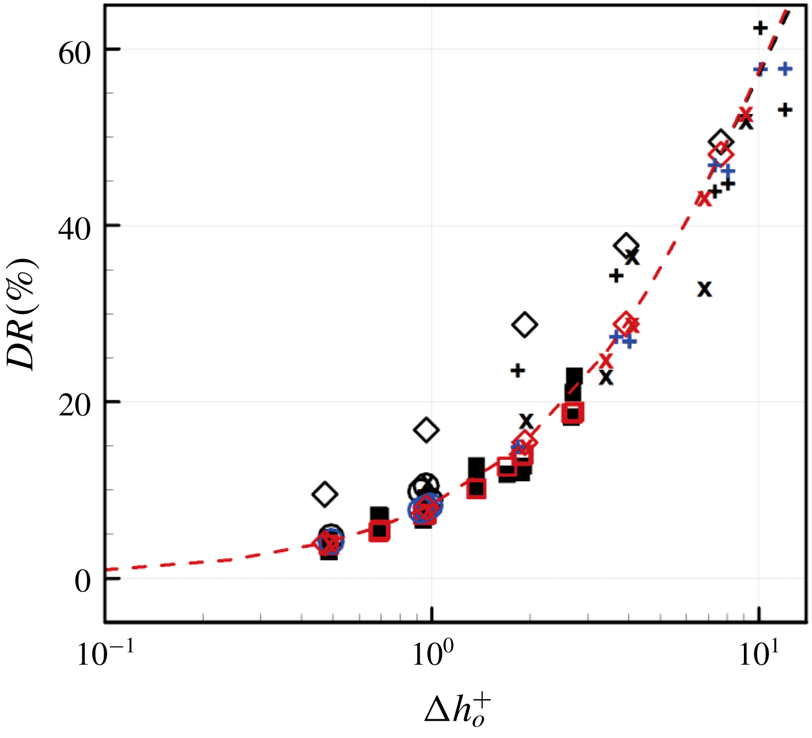Here, we select the cases of LIS and SHS with longitudinal grooves, and take $\tanh (\unicode[STIX]{x03C0}D/L_{g})\approx 1$ for the data from the DNS with shear-free boundary condition at the interface. The comparison of these data with the predictive model is made in figure 11. As shown, the model agrees very well with the data from the present and other studies, except for those from Türk et al. (Reference Türk, Daschiel, Stroh, Hasegawa and Frohnapfel2014), indicating that (4.9) with (4.2) and (4.3) is a predictive model for drag reduction by SHS and LIS.

Figure 11.

Drag reductions from DNS (SHS and LIS) and prediction by (4.9) with (4.2) and (4.3) with $\unicode[STIX]{x0394}h_{o}^{+}(=b_{x,eff_{o}}^{+}-b_{z,eff_{o}}^{+})$ : ▪ and ▫, present study; ○ (black) and ○ (blue), Fu et al. (Reference Fu, Arenas, Leonardi and Hultmark2017);  $+$ (black) and $+$ (blue), Park et al. (Reference Park, Park and Kim2013);  $\times$  (black) and $\times$  (red), Rastegari & Akhavan (Reference Rastegari and Akhavan2015, Reference Rastegari and Akhavan2018); ♢ (black) and ♢ (red), Türk et al. (Reference Türk, Daschiel, Stroh, Hasegawa and Frohnapfel2014); - - - (black) and - - - (red), equations (4.9) and (4.10) with $c_{f_{o}}=0.0083$ , respectively. Here, the black- and red-coloured symbols are from DNS and predicted ones, respectively.

Table 8.

Predicted effective slip lengths and drag reductions for $Re_{\unicode[STIX]{x1D70F}_{o}}\approx 395$ (heptane).