Notation

1. Introduction

In Alpine terrain, redistribution of snow by wind is a major factor in snow pack evolution as well as in the formation and effectiveness of avalanches. Thus, it is of great interest to predict snow redistribution and its influence on avalanche danger with regard to avalanche forecasting and land-use planning.

Avalanche warning on a regional scale requires information on the occurrence of snowdrift and on the (new-) snow distribution on a mesoscale (several 10 km²). Scarcity of land resources is a major restricting factor in the economic development of many mountain villages. In these villages, avalanche danger often causes restrictions on land use. As great interest exists in using all available land resources, efforts are made to develop numerical avalanche models to reliably determine endangered zones. These models require highly resolved input data on the snow-mass distribution in avalanche release zones (microscale; several 100 m²) which depends strongly on snowdrift. In both cases, one is interested in suitable tools to assess, analyze or forecast the effect of blowing and drifting snow in Alpine topography. Corresponding to World Meteorological Organization (WMO) standard observations, the term drifting snow is used to describe the near-surface wind transport, whereas the expression blowing snow is reserved for situations where particles rise to a height of 1.8 m and above. However, in the following the term drifting snow or wind transport will be used to refer synonymously to both phenomena.

The snowdrift model presented here is based on many previous field studies of snow transport as well as on physical and numerical simulations for aeolian particle transport. The field studies show that snow transport is basically given by the transport in saltation and in suspension (Reference KobayashiKobayashi, 1972; Reference RadokRadok, 1977; Reference TakeuchiTakeuchi, 1980; Reference SchmidtSchmidt, 1982, Reference Schmidt1986; Reference Mellor and FellersMellor and Fellers, 1986). These studies were carried out on plains and aimed at determining the transport rate for steady-state conditions. The attained empirical formulations show that transport rate is proportional to a power of the wind speed, where the power varies typically between 2 and 4. Only a few attempts have been made to measure snowdrift in mountain areas (e.g. Reference FohnFöhn, 1980; Reference Schmidt, Meister and GublerSchmidt and others, 1984; Reference MeisterMeister, 1987) where drift flux measurements were made on a crest. Reference Fohn and MeisterFöhn and Meister (1983) also measured the spatial distribution of snow in the area surrounding a crest. Similar measurements were made by Reference CastelleCastelle (1995) for a mountain pass. Physical simulations have been used to study the deposition patterns around obstacles (e.g. Reference IversenIverson, 1980; Reference AnnoAnno, 1985) or have dealt with particular features of the drift process (e.g. the particle–bed impact as studied by Reference Maeno, Araoka, Nishimura and KanedaMaeno and others (1979, Reference Maeno1985, Reference Maeno, Nishimura, Sugiura and Kosugi1995), Reference Willets, Rice and Barndorff-NielsenWillets and Rice (1985), Reference Rice, Willets and McEwanRice and others (1995, Reference Rice, Willets and McEwan1996) and Reference Nishimura, Sugiura, Nemoto and MaenoNishimura and others (1998). Numerical models of snow or sand drift differ widely in scope and focus. Specific processes have been studied, for example, simulating the grain impact (Reference Werner and HaffWerner and Haff, 1988) or particle transport in saltation (Reference Anderson and HaffAnderson and Haff, 1988, Reference Anderson and Haff1991; Reference WernerWerner, 1990; Reference McEwan and WilletsMcEwan and Willets, 1991; Reference SorensenSørensen, 1991). Also models based on heuristic rules for avalanche forecasting have been developed, like ELSA (Reference Mases, Buisson, Frey and SivardièreMases and others, 1995).

Most transport models for snow can be classified into two categories: Eulerian–Lagrangian (e.g. Reference Sato, Uematsu, Kaneda, Izumi, Nakamura and SackSato and others, 1997; Reference Sundsbø, Hansen, Izumi, Nakamura and SackSundsbo and Hansen, 1997) or Eulerian–Eulerian (Reference Uematsu, Kaneda, Takeuchi, Nakata and YukumiUematsu and others, 1989; Reference Liston, Brown and DentListon and others, 1993). However, Reference Masselot and ChopardMasselot and Chopard (1998) follow a different approach, using a lattice Boltzmann model. Particle tracking, which is done in the Eulerian–Lagrangian approach, can require large computational effort and restrict the application of those models to small areas (e.g. the estimated number of particles in the saltation layer is about 1–5 × 10⁶ m⁻²). All the models discussed above are two-dimensional. More recent models address the requirements of three-dimensional transport modeling (Reference Liston and SturmListon and Sturm, 1998; Reference Naaim, Naaim-Bouvet and MartinezNaaim and others, 1998). These models are Eulerian–Eulerian. Common to most transport models is the separation between saltation and suspension. Either the transport rate for suspension is defined by a height integration of the flux with given profiles for the wind speed and concentration (Reference PomeroyPomeroy, 1989; Reference Liston and SturmListon and Sturm, 1998), or a separate balance equation for the particle concentration is solved (Reference UematsuUematsu, 1993; Reference Naaim, Naaim-Bouvet and MartinezNaaim and others, 1998). The assumption that the wind profile develops fully into a logarithmic profile over the total height of the suspension layer, which Reference PomeroyPomeroy (1989) and Reference Liston and SturmListon and Sturm (1998) take for granted, is critical in Alpine terrain. For example, measurements (Reference FohnFöhn, 1980) show that the wind profile on a crest is very different from a logarithmic profile. This difference also affects the concentration profile. Almost all descriptions of the transport in saltation (e.g. Reference PomeroyPomeroy, 1989; Reference UematsuUematsu, 1993; Reference Liston and SturmListon and Sturm, 1998; Reference Naaim, Naaim-Bouvet and MartinezNaaim and others, 1998) rely on Reference PomeroyPomeroy’s (1989) empirical formulation, which is defined for steady-state conditions. Reference Pomeroy and GrayPomeroy and Gray (1990) assume that it takes about 300–500 m for a boundary-layer flow that is approximately 3 m in depth to reach steady conditions. In Alpine terrain, with its high variability, 300–500 m is a long distance. Reference CastelleCastelle (1995) pointed out that the drift transport seldom if ever reaches steady state in mountainous terrain. Recently, attempts have been made to parameterize the deviation from steady state (Reference Liston and SturmListon and Sturm, 1998; Reference Naaim, Naaim-Bouvet and MartinezNaaim and others, 1998).

Due to the limited range of applicability because of the simplifications that were used, the above models cannot accurately represent complex topographies like an Alpine terrain and non-steady wind fields. To overcome some of the weaknesses of the previous models, the model presented here uses a different approach for the description of saltation. Based on particle motion, a continuum formulation is derived for the saltation layer. This formulation includes deposition and erosion, distinguishing between aerodynamic entrainment and particles ejected due to impact, and does not require steady-state conditions.

2. Numerical model

Blowing and drifting snow is strongly related to the atmospheric boundary layer (ABL). Erosion, transport and deposition of snow depend on the wind field and the turbulence within the lowest 10–100 m of the boundary layer, the so-called surface layer (SL). It is widely accepted that the primary transport mechanisms are saltation and suspension. The transport due to saltation usually starts at light wind speeds, M ₁₀ = 5–8 m⁻², where M ₁₀ is the wind speed at 10 m (Reference SchmidtSchmidt, 1980; Reference CastelleCastelle, 1995; Reference Li and PomeroyLi and Pomeroy, 1997). Typical transport rates (integrated over the height) range from 0.001 to 0.03 kg m⁻¹ s⁻¹ (Reference TakeuchiTakeuchi, 1980; Reference CastelleCastelle, 1995). Saltation is usually restricted to a vertical extension of about 0.01–0.1 m (Reference KobayashiKobayashi, 1972), and drift densities range from 0.1 to 1 kgm⁻³ (Reference Mellor and FellersMellor and Fellers, 1986; Reference Pomeroy and GrayPomeroy and Gray, 1990; Reference CastelleCastelle, 1995). For comparison, even if the transition from saltation to suspension is more or less continuous, noticeable suspension starts at moderate wind speeds (M ₁₀ = 7–11 m⁻²), depending on the particle size and flow turbulence. An estimation of the required shear velocities is given in Reference GauerGauer (1999). The typical mean grain-size in drifting snow is about 150–200 µm (Reference SchmidtSchmidt, 1984; Reference PopePope, unpublished). Transport rates for suspension range from 0.01 to 0.1 kg m⁻¹ s⁻¹ and drift density is <1 kg m⁻³ (Reference Mellor and FellersMellor and Fellers, 1986; Reference CastelleCastelle, 1995). The vertical extension can reach several tens of meters, though the drift density usually decreases significantly with increasing height above the surface.

For a review of current conceptual understanding of aeolian particle transport, the reader is referred to Reference Anderson, Sørensen and WilletsAnderson and others (1991) or Reference McEwan, Willets and PyeMcEwan and Willets (1993). In a greatly simplified form, one can imagine the transport due to blowing and drifting snow as follows (see also Fig. 1): If the wind blowing over a snow surface becomes sufficiently strong, and wind shear exceeds a certain critical value, the so-called threshold, some grains are set in motion by the wind. Initially, only a few of these will be lifted off the surface and accelerated by the wind. Some of them will gain enough energy to rebound and/or eject other grains on impact. At the onset, the number of grains resulting from an impact, the so-called mean replacement capacity, is more than one on average. This results in an exponential increase of grains in the saltation layer, which follow more or less ballistic trajectories determined by the time-averaged wind profile. Grains within the saltation layer are not — or only weakly — influenced by turbulence of the wind. As more and more grains saltate, the vertical wind profile changes due to the considerable extraction of momentum from the airflow by the grains in motion. Now the grains gain less energy, and the probability of a grain rebounding and/or ejecting other grains on impact decreases until the mean replacement capacity reaches the equilibrium value of one. At this stage, the number of saltating grains fluctuates around a certain value, sometimes called the saturation value, which depends on the driving-wind field and certainly on the properties of the snow surface. The surface properties determine the fluid threshold as well as rebound and dislodgements effected by collisions of grains with the surface, and thus play an important role in saltation. In turbulent and gusty winds, a certain number of particles will be caught by eddies and will travel a significantly greater distance without surface contact. The ratio between mass transport by suspension and mass transport by saltation increases with increasing wind speeds and turbulence. In all cases, gravity counteracts the wind forces on the grains in saltation and suspension.

Fig. 1.

Schematic diagram of the processes involved in snowdrift. M(z), wind speed at a given height z; τ, shear/Reynolds stress; τ _c , critical shear stress; J _cae , aerodynamic entrainment; J _cej , ejection rate; J _cd , deposition rate; J _ct , turbulent entrainment; J _cs , settling rate due to gravity; J _m , horizontal mass-transport rate; J _pr , precipitation rate. The acceleration of grains causes a modification of the wind profile.

In short, wind transport can be regarded as the result of five closely/mutually linked processes:

1. aerodynamic entrainment,

2. grain trajectories,

3. grain–snowpack impacts,

4. modification of the wind field,

5. transport due to turbulent suspension.

In the following, a numerical model is proposed that uses a continuum mechanical approach to describe blowing and drifting snow, and makes use of a splitting of the two dominant transport processes into two mutually coupled layers. This procedure is chosen to reduce the computational effort, which would drastically increase if the saltation layer was to be fully resolved. The transition mode between saltation and suspension, the so-called modified saltation, is not separately considered and it is assumed that those particles are either in the saltation layer or in suspension. The complete derivation for the model is given in Reference GauerGauer (1999).

2.1. Wind-field and suspension modeling

As outlined above, the driving force for wind-drifting snow is the airflow within the surface layer. This flow can be described using the equation of state (1), and the conservation equations for mass, momentum (3), moisture (4) and heat (5). For atmospheric flows smaller than meso-γ-scale (≪ 12 km), the conservation equation for mass usually reduces to the incompressibility approximation (2). Note that Einstein summation notation will be used in the following. In Equations (1–5), all unprimed quantities are to be understood as Reynolds averaged quantities.

(1)

(2)

(3)

(4)

(5)

In Equation (4), q _T denotes the total specific humidity of air, which can be split into a vapor and a non-vapor part, using q _T = q + q _L. The heat balance (Equation (5)) is expressed in terms of the potential temperature, . The virtual temperature, T _v, is defined as the temperature at which dry air must be in order to have the same density as moist air at the temperature T. It is given by

(6)

where r is the mixing ratio, and r _sat and r _L are the saturation and solid/liquid water mixing ratios, respectively. By substituting Equation (6) into Equation (1), effects of mass concentration on the wind flow can be taken into account. For a complete derivation of these equations, the reader is referred to the literature (Reference PichlerPichler, 1986, Reference StullStull, 1997). In the following, it will be assumed that temperature effects, sublimation and effects due to the Coriolis term, f _c ∊_{ij 3} u_j , are negligible for the present purpose of the model. It is assumed that snow grains travel with a velocity , where W _f is the absolute value of the free-fall velocity of a grain. This assumption implies that all grains have the same size. On the conditions above, Equation (5) is negligible, a fixed reference temperature, T _ref, can be used, and Equation (4) can be replaced by the balance equation for only the solid part,

(7)

to describe precipitation as well as the suspension transport. The solid part of the moisture can be written as q _L = cρ _p /ρ _a, where c is the volume fraction of snow and ρ _p is the intrinsic density of ice. On the righthand side of Equation (7), a sink/source term for the phase change due to sublimation is neglected. The sublimation rate of an ice particle is determined by the difference between the saturation vapor pressure over ice, as a function of the particle radius, and the water-vapor pressure of the ambient air. At the present stage, the model will be used to represent the redistribution of snow during precipitation events with a relative humidity of approximately 100%. In this case, it is reasonable to assume that the difference in the vapor pressures is small and hence the sublimation loss negligible. Otherwise, the sublimation rate must be parameterized (as in Reference Liston and SturmListon and Sturm, 1998), or in a consistent manner the phase exchange, −E/ρ _a, must be included on the righthand side of Equation (7) and an additional equation for the vapor part is needed. As phase exchange depends on the grain-size, the grain-size distribution should be considered. Also the latent-heat transfer should be taken into account, so that Equation (5) is no longer negligible. The particle temperature, which determines the saturation vapor pressure, is influenced by the absorbed solar radiation. This fact as well as Equation (5) require an approximation of the incoming solar radiation.

For turbulent closure, the well-known e–∊ model is used (see, e.g., Reference RodiRodi, 1980).This was first used in a snowdrift model by Reference Liston, Brown and DentListon and others (1993) in their two-dimensional model, and has been used to simulate boundary-layer evolution, flow changes in roughness and topography, and sea-breeze fronts (Reference StullStull, 1997). It is a one-and-a-half-order closure and is used as a compromise between accuracy and effort. Here, Reynolds stress and Reynolds flux are approximated by

(8)

and

(9)

where the turbulent viscosity is parameterized by

(10)

Separate balance equations are formulated for the turbulent kinetic energy, e, and the dissipation rate, ∊, i.e.

(11)

and

(12)

The empirical constants are set to c_µ = 0.09, c _{1 ∊} = 1.44, c _{2 ∊} = 1.92, σ _T = 0.9, (σ _e = 1.0 and σ_∊ = 1.3 (Reference RodiRodi, 1980).

The description of the suspension layer above is similar to simple mixture formulations used in the description of passive tracers and in air-pollution modeling. As in those models, momentum transfer between the different phases is assumed negligible. However, mass change due to the suspension of snow is included here. Reference Naaim, Naaim-Bouvet and MartinezNaaim and others (1998) used a slightly modified e–∊ for their snowdrift model to account for the effect that particles have on turbulence.

2.2. Saltation-layer modeling

Within the saltation layer, the assumption of a negligible momentum transfer breaks down, as the acceleration of massive grains exerts an additional force on the wind. Hence, within the saltation layer, the mass balance and the momentum balance are formulated for each of the two phases, dry air and snow. Scaling analysis (Reference GauerGauer, 1999) shows that mass conservation within the saltation layer is primarily determined by the conservation of the snow mass

(13)

and that the reduced mixture momentum equation describes the balance of the force necessary to accelerate the saltating particles and the driving forces, represented by the Reynolds/ shear stress and gravity. Therefore,

(14)

where ρ _d is the density of dry air. In the numerical model, the following discretized volume-averaged versions of Equations (13) and (14) are used

(15)

and

(16)

where sub/superscripts 〈1〉, 〈2〉, 〈3〉, 〈4〉, 〈5〉 and 〈6〉 stand for the direction of the control volume in x, y, z, −x, −y and −z, respectively, and are the approximated slope-parallel acceleration acting on a rebounding or ejected grain, respectively, during its jump, and c _R and c _E are the corresponding parts of the volume fraction of snow, c, within the saltation layer. Let us assume that the ratio of rebounding and ejected grains in a control volume will remain unchanged due to advection during a time-step. In this case,

(17)

and

(18)

where and are the calculated particle concentrations of rebounding and ejected particles, respectively, from the previous time-step. The advection coefficients are given by

(19)

where , denotes the vector of the mean particle velocity and are the area vectors of the sides in the direction k of the control volume. The volume V is approximated by A^〈6〉 h _s, where A ^〈6〉 is the surface area and h _s is the saltation height. A parameterization of ,h _s, , etc., will be defined later on.

2.2.1. Concentration exchange between saltation and suspension layer

The settling due to gravity, J _cs, and the turbulent entrainment, J _ct, determine the boundary conditions of the concentration exchange between the saltation layer and the suspension layer. Grains settle out of the suspension layer through the boundary area, A^〈3〉, at velocity . Turbulent fluctuations will also influence the settling. On the other hand, grains in the saltation layer can be caught by turbulent eddies and lifted off, and then transported by the mean flow. For the description of the mass exchange the following statement is used:

(20)

(21)

where A _〈3〉 is set to

(22)

and c _〈3〉 is given by

(23)

and the diffusion coefficient describing the turbulent dispersion is set to

(24)

n_i is the normal vector to the boundary area between the saltation layer and the suspension layer, is the area vector. , is the wind velocity at the saltation-layer height and c _s is the volume fraction of snow in the suspension layer above. The value is obtained by similarity theory for the neutral boundary layer and corresponds to the vertical fluctuation velocity (Stull, 1987). The statement for the mass exchange is adapted from a hybrid differencing scheme in which central differencing is used if the mesh Peclet number (C/D) is < 2, and upwind differencing, neglecting diffusion, is used if the mesh Peclet number is > 2.

2.2.2. Erosion and deposition

Although Reference BagnoldBagnold (1954), in one of the first thorough examinations of the drift processes, recognized the difference between fluid threshold and impact threshold, most models do not distinguish between aerodynamic entrainment and ejecta due to impact. Reference Anderson, Sørensen and WilletsAnderson and others (1991) as well as Reference McEwan, Willets and PyeMcEwan and Willets (1993) emphasized the importance of the impact process for particle entrainment, and it is observed that threshold wind speeds are significantly reduced if there are already snow grains in the air.

The mass exchange between the snowpack and the saltation layer is determined by erosion and deposition of snow grains. As mentioned above, two different mechanisms are important for erosion: aerodynamic entrainment and particle impact. At present, little is known about the exact nature of either mechanism in the case of snow. In the absence of better knowledge on aerodynamic entrainment, the statement proposed by Reference Anderson and HaffAnderson and Haff (1991) is adopted, i.e. a linear relation between the number of entrained grains per unit area and unit time, N _ae, and the excess shear stress is used. Thus,

(25)

where τ _a is the so-called airborne shear stress and is assumed to be equal to the shear stress of the airflow at the bed, τ _c is the critical fluid shear stress for entrainment and ζ is an empirical constant. As no value is known for the case of snow, ζ = 10⁵ grains N⁻¹ s⁻¹ is used, which is the value used by Anderson and Haff for sand. Actually, the choice of ζ is not that important, as fluid entrainment essentially acts during the initial development of wind transport. Once there are some particles in transport, they act as seeding agents for further dislodgements. The impacts between these particles and the surface eject more particles, leading to a cascade as mentioned above. This cascade drives the transition from an aerodynamically controlled to an impact-controlled system. More important is the choice of τ _c, which determines the onset of drift, at least during periods without additional precipitation. τ _c is highly dependent on the snowpack properties and meteorological conditions such as particle size and shape, bonding, temperature and humidity. Reference SchmidtSchmidt (1980) tried to estimate τ _c for wind conditions over a flat snow surface. According to him, values for τ _c range from 0.04 to 9000 Pa. In comparison, typical values for the wind shear stress/Reynolds stress, τ _a, during snowdrift vary from 0.06 to 1 Pa, indicating that aerodynamical entrainment is only possible within a small range. The lower end of the estimation above is in agreement with observations based on the onset of drift (see, e.g., Reference CastelleCastelle, 1995; Reference Li and PomeroyLi and Pomeroy, 1997). Little is known about the influence of snowpack properties and meteorological conditions on τ _c. Reference Li and PomeroyLi and Pomeroy (1997) show a relation between air temperature and the mean threshold wind speed. An attempt to relate the threshold to snowpack properties, such as particle size, sphericity and dendricity, can be found in Reference Guyomarc’h and MérindolGuyomarc’h and Mérindol (1998).

The erosion due to particle impacts is determined by the number of particle impacts per unit time on the snow surface and the number of ejected particles per impact. The impact rate is given by

(26)

where V _p is the particle volume and t _J is the average duration of a particle jump. To estimate the number of particles ejected per impact, N _EpI, it is reasonable to assume that this number is a function of the difference of the kinetic energy of a particle before the impact, E _I, and after it, E _R, of the total kinetic energy of the ejected particles, N _EpI E _E, of the energy dissipated into the bed during the impact, E _D, and, if cohesion is included, of the total energy of the bonds, N _EpI E _B, which had to be broken. From the energy balance, we obtain

(27)

All these energies can be expected to depend on the mechanical properties of the snowpack, but the exact relationship is as yet unknown. To estimate a value for N _EpI, some assumptions are made. The assessment for E _D was based on the numerical simulations of Reference Anderson and HaffAnderson and Haff (1991) who found that, in the case of sand (E _B = 0), the mean number of ejecta increases approximately linearly with the impact speed, where the ejection rate N _EpI ≈ 1.5 m⁻¹ s ||U _I||. For the assessment of E _I, E _R and E _E see Table 1. Figure 2 shows an approximation of the ejection rate with E _B as parameter. The range of E _B from 10⁻¹⁰ to 10⁻⁸ J seems to be reasonable regarding different snow types (Reference SchmidtSchmidt, 1980; Reference GublerGubler, 1982). Using Equations (26) and (27), the ejection rate can be expressed as

(28)

Fig. 2.

Approximation of the ejection rate for snow particles due to particle impact as function of the impact speed for different values of the bonding energy, E _B .

Here and in Equations (29) and (30), there is a distinction between rebounding particles and those particles which were just ejected because their respective impact speed U _I and jump time t_J are significantly different. Both kinds are marked by subscript ()_R and ()_E, respectively.

Table 1.

Typical values of the quantities characterizing the particle–bed impact

Snow grains in saltation tend to rebound at the surface. On the other hand, if a snow grain does not rebound it will be deposited at the surface. Hence, if P _R is the probability that a snow grain will rebound on impact, 1−P _R is the probability that it will be deposited. Thus, the deposition rate can be described by

(29)

Physical simulations (Reference Kosugi, Nishimura and MaenoKosugi and others, 1995; Reference Rice, Willets and McEwanRice and others, 1995, Reference Rice, Willets and McEwan1996) show that the probability of a particle rebounding is approximately 0.6–0.9 for the investigated impact speeds. In the absence of better data, the relation

(30)

is used, which Reference Anderson and HaffAnderson and Haff (1991) proposed for sand. Assuming that the rebound probability for a snow grain at the surface of a snowpack is smaller than for a sand particle on a bed of sand, the coefficient ξ is set to 1.5 m⁻¹ s instead of the original value, 2 m⁻¹ s. Actually, the rebound probability is expected to depend on the snowpack properties, but little is known about the relationship as yet.

2.2.3. Modification of the wind field

Reference BagnoldBagnold (1954) was the first to note the feedback between particle movement and the driving wind. Thereafter, it became common to parameterize the interaction between the particles in the saltation layer (extraction of momentum) and the wind above, using an increased roughness length, z ₀, in the equation for the logarithmic wind profile

(31)

Reference OwenOwen (1964) assumed that the saltation-layer height scales as and that the roughness length can be given by

(32)

However, there are two weak points. First, it is unreasonable to assume that the roughness length depends only on the saltation-layer height and that there is no dependency on the number of particles within the saltation layer. This oversimplification might explain why there is a large difference in the reported values for the constant k. Owen proposed k = 0.02, whereas Reference Rasmussen, Sørensen, Willets and Barndorff-NielsenRasmussen and others (1985) reported values of 0.14 and 0.18, and Reference Pomeroy and GrayPomeroy and Gray (1990) set k to 0.1203. Second, Equation (31) cannot represent the rapid decrease in the wind speed just above the top of the saltation layer (h _s ≈ 1–2 cm), an effect which can be observed, for example, in Bagnold’s classical wind-velocity plot (Reference BagnoldBagnold, 1954, fig. 17).

The primary effect that the particles have on the airflow is to provide a spatially distributed momentum sink, with sink strength dτ _a(z)/dz ≅ −dτ _g(z)/dz per unit volume of fluid. τ _a(z) is the flux of fluid momentum across the level z, and τ _g(z) represents the net flux of slope-parallel grain momentum across that level. dτ _g(z)/dz corresponds to the interaction (drag) forces on the wind, due to the slope-parallel acceleration of the grains by the air. This acceleration mainly takes place within the saltation layer. The total shear stress is given by

(33)

where is the stress at the top and above the saltation layer. Vegetation canopies have a similar effect on flow. In boundary-layer meteorology, it is customary to describe the effect of vegetation on the flow above by a generalized logarithmic law (Reference ThomThom, 1971; Reference JacksonJackson, 1981; Reference WieringaWieringa, 1993). In such a case,

(34)

where d is the displacement height and z ₀ is the roughness length. According to Reference ThomThom (1971) and Reference JacksonJackson (1981), z ₀ expresses the magnitude of forces acting on the surface, whereas d is related to the distribution in z of these forces. Hence, for a known distribution of the interaction (drag) forces within the saltation layer, F _DW(z), the displacement height can be calculated according to the statement of Reference Shaw and PereiraShaw and Pereira (1982):

(35)

where and τ _a are the airborne stresses at the top of the saltation layer and at the surface of the snowpack, respectively. Assuming that the particles do not influence each other, the interaction force can be written as

(36)

where N(z) is the number of particles in a height z with a slope parallel to the relative velocity . C _D is the drag coefficient and d _P is the grain diameter. In Equation (37), only the acceleration of the grains due to the wind is represented. The reverse transfer of momentum due to descending grains from faster flow levels causes an enhancement of the air velocity close to the surface. This departure from the logarithmic wind profile within the saltation layer is observed, for example, by Reference BagnoldBagnold (1954) and is also reported by Reference Maeno, Araoka, Nishimura and KanedaMaeno and others (1979). For the parameterization, this departure is taken into account, as discussed in the following subsection.

For the description of the roughness length, the following statement is used:

(37)

where z _0s is the aerodynamic roughness length for a snow cover without saltation, typically in the range 10⁻⁴ to 10⁻³ m (Reference StullStull, 1997, p. 380), here set to 3 × 10⁻⁴ m, and, in the absence of data for snow transport, λ is assumed to be 0.1, a value used for vegetation. Equation (34) is used as a boundary condition for the wind speed, at the interface between the saltation and suspension layers (see section 2.4), assuming that, at least in the lowest part of the suspension layer, a logarithmic profile exists.

2.3. Parameterization

To close the system of equations for the saltation model, h _s, d, , , etc., must be determined.

The transport within the saltation layer is regulated by the motion of saltating grains, bouncing off the snow surface and following ballistic trajectories. It is widely accepted that the saltation trajectories are governed by the following relation:

(38)

where the terms on the righthand side denote the gravitational force (I), the drag force (II), the lift force (III), Magnus force (IV), added mass force (V), pressure-gradient term (VI), electrostatic force (VII) and the Basset history term (VIII) (for reference see, e.g., Reference Clift, Grace and WeberClift and others, 1978, ch.11; Reference Schmidt, Dent and SchmidtSchmidt and others, 1998). With the aid of an appropriate scale analysis (Reference GauerGauer, 1999), it can be shown that, in a first approximation, Equation (38) reduces to a balance of inertial, drag and gravity forces, such that:

(39)

where U_ϱi is the relative velocity between the particle and the airflow (U_ϱi = U_Pi – u_i ). These equations form a system of differential equations which can be solved for given initial conditions, U_{P 0i} , and a known wind field, u_i . They build the basis for parameterization of the saltation layer.

Physical simulations with sand and snow (Reference Kosugi, Nishimura and MaenoKosugi and others, 1995; Reference Rice, Willets and McEwanRice and others, 1995, Reference Rice, Willets and McEwan1996; Reference Nishimura, Sugiura, Nemoto and MaenoNishimura and others, 1998), as well as numerical simulations (Reference Werner and HaffWerner and Haff, 1988; Reference Anderson and HaffAnderson and Haff, 1991) of the particle–bed impact, have been carried out. All these studies confirm that impacting particles behave in similar ways, in that they have a certain probability to rebound, and that the mean impact, launch angles, and ratio of impact to rebound velocity vary only over a small range. Ejected particles also behave in a specific manner. Typical values of the quantities describing the particle–bed impact are shown in Table 1 (for notation see Fig. 3).

Fig. 3.

Sketch of grain impact: a particle with velocity U _I impacts at angle α _I on the snowpack and rebounds with velocity U _R and at angle α _R . In addition, a particle may be ejected with velocity U _E at angle α _E .

ς _R, ς _E, α _R, and α _R describe the particle–snowpack interaction on impact (e.g. ς _R characterizes the energy loss of a rebounding grain on impact). All these parameters are expected to be affected by the mechanical properties of the snowpack, but little is known about the relationship as yet. For our parameterization, the following values are chosen: ς _R = 0.5, ς _E = 0.1, α _R = 40° and α _E = 65°. Furthermore, within the saltation layer the similarity assumptions are made, i.e. the airflow velocity, u_i , and the concentration, c, maintain approximately similar profiles in the z direction (perpendicular to the surface) as they change in time or in the x and y directions. In particular, it is assumed that

(40)

(41)

where ξ_u = [1 + ς(1 − z/h _s)]⁻² with ς = 0.35, and ξ _c = 1 is assumed. Based on the assumptions above and on Equation (39) as well as on values given in Table 1, it is possible to calculate the trajectory of a single grain. To be consistent, the determination of the wind field within the saltation and the particle trajectories should be carried out simultaneously. The use of the profile function (Equation (40)) is a simplification, where it is assumed that the momentum extraction and the modification of u_i , due to the particles is similar to the case of vegetation. Figure 4 shows an example of such a calculation. Here, the normalized horizontal velocity of a rebounding particle is presented as a function of the normalized height for the ascending as well as the descending branch of the trajectory. The mean horizontal velocity, , and the assumed wind profile within the saltation layer are also shown. The mean particle velocity is approximately . Calculations with varying show similar results. In the saltation model, is set to 0.58 . The other missing parameters of the particle trajectories (e.g. h _s, d, , etc.,) can also be determined in this way. Figure 5 presents those parameters as functions of for a rebounding grain. Similar calculations were used to determine the corresponding quantities for ejected grains.

Fig. 4.

Normalized slope horizontal particle velocities as a function of the normalized height for a rebounding grain, α _R = 40°, and ; ascending U _p ↑, descending U _P ↓, mean and the wind speed, u.

Fig. 5

Trajectory parameters as functions of the wind speed at the top of the trajectory, for rebounding grains ( , α _R = 40°). (a) Hop/saltation layer height, h _s , as a function of . (b) Horizontal acceleration, ,as a function of . (c) as a function of .

2.4. Implementation

The model is implemented in the commercial flow solver CFX4.1 from AEA Technology, England (AEA Technology, 1995). This program is based on the finite-volume technique and uses a body-fitted grid which can be modified during the calculation. Thus the modification of the topography due to deposition and erosion of snow can be modeled. So-called Fortran user routines provide the programming interface for problem-specific modifications of the code and have proved flexible enough to accommodate all the extra computations for the simulation of blowing and drifting snow. Hence, the program serves as a framework, providing the solver for the wind field and for the suspension mode, whereas the calculations of the saltation mode were embedded in Fortran routines. Although the wind field, suspension and saltation form a mutually coupled system, here a certain decoupling was desired. The wind field and the suspension mode are solved together and provide the boundary condition for the saltation-layer calculation, which is carried out between two time-steps. On the other hand, the boundary conditions for the next time-step were obtained from this calculation. In order to evaluate the snowpack, the grid is adjusted to the new-snow depth at regular time intervals. For that purpose, at every time-step ΔHS _i is calculated according to

(42)

where ΔHS_e is the remaining erodible snow depth and c _λ is the volume fraction of snow in the snowpack. After a certain number of time-steps, n, the grid is adjusted to the new-snow depth:

(43)

3. Field measurements and simulation results

To test the model, two methods were pursued. Firstly, the model was compared with experimental results described in the literature. Secondly, it was tested against data from the Gaudergrat experimental site in the Swiss Alps.

Reference KobayashiKobayashi’s (1972) are one example of measurements reported in the literature. Figure 6 shows a comparison between his field experiments and drift simulations. The mass flux, Q, is plotted against the wind speed at 1 m. Kobayashi noted that due to the scattering in the drift rate, especially at low wind speeds, no distinct threshold wind speed for the occurrence of snowdrift was found, but it was in the range 4–6 m s⁻¹. For the simulation, τ _c was set to 0.05 Pa, and E _B was assumed to be 10⁻⁹ J. Taking into account the uncertainties in the snowpack properties, the simulation and the measured data are in good agreement.

Fig. 6.

Snowdrift rate as a function of the mean wind speed, M (z = 1 m). Comparison between simulation (− + −) and measurements done by Reference KobayashiKobayashi (1972): ⊕ without snowfall; ● with snowfall.

A logarithmic plot of the simulated steady mass flux vs M ₀.₂₅ is given in Figure 7. At low reference velocities, a rapid increase in the mass flux can be observed. Then the rate of increase diminishes with increasing M _0.25, but is still non-linear. The power decreases from approximately 4 to 2 with increasing wind speed. This decrease indicates that with increasing wind speed a saturation of transport occurs. The power range agrees quite well with those of empirical formulations given in the literature (Reference KobayashiKobayashi, 1972; Reference TakeuchiTakeuchi, 1980; Reference SchmidtSchmidt, 1982, Reference Schmidt1986; Reference Nishimura, Sugiura, Nemoto and MaenoNishimura and others, 1998). The fit in Figure 7 corresponds to a power of approximately 3, an oft-found value in empirical formulations. A separate comparison between measured and simulated drift rates in saltation shows that the model reproduces these rates quite well (Reference GauerGauer, 1999).

Fig. 7.

Logarithmic plot of the simulated steady-state mass flux against the logarithmic M_0.25 showing the non-linear behavior. The dotted line represents the fit log(Q) ∝ 3.1 log(M _0.25).

In the next step, the model was applied to the Gaudergrat experimental site for a full-scale simulation of an Alpine crest. Gaudergrat ridge, 2 km north of Weissfluhjoch/Davos, has a rather sharp crest — the slope angles range from 28° to 38° — and might be regarded as prototypical of Swiss Alpine topography. The prevailing wind direction during strong precipitation periods is more or less northwest and thus perpendicular to the crest line. Up to now, field measurements of drifting snow in complex terrain are rather scarce, and, although the wind as driving force is of major importance, no example is known where the wind field and the snow distribution have been simultaneously measured. In winter 1996/97, the ridge was equipped with five wind masts in the surrounding area (M78, M76, M75, M74/73 and M72) to obtain a good impression of the wind field around the crest during interesting snowdrift periods. In addition, meteorological and snowpack parameters were measured on both sides of the ridge (M77 and M74/73). Figure 8 shows the locations of the installed masts and the slope angles at the ridge. A complete description of the experimental site and the measurements can be found in Reference GauerGauer (1999).

Fig. 8.

Slope-angle map of the Gaudergrat experimental site showing locations of the masts MXX and the hut that housed the transmitting equipment. The box marks the area of the numerical simulations. (Topographic data DHM25: © Swiss Federal Office of Topography.)

For comparison with the simulations, the spatial snow redistribution was measured by soundings of the snow depth before and after a drift episode along five equidistant lines across the crest, roughly 8.5 m apart and > 200 m long. The soundings were taken at 4 m intervals along the lines; in the neighborhood of the crest this distance was reduced. Thus, every field campaign resulted in around 350 data points. All measurement points were marked by thin bamboo stakes during the first campaign, so later measurements could be taken at the same points (with an estimated horizontal deviation of < 0.1 m). In this manner, uncertainties in the depth measurements due to the small-scale topography were minimized. The settling of the snowpack, different for south and north aspects, between two successive soundings was taken into consideration. For this purpose, small pits were dug at several points of both slope sides, and the snow density was measured, and all new-snow depths are recalculated for the average new-snow density (110 kg m⁻³). For the comparison with the simulation these new-snow depths are normalized with HN_ref, where HN_ref is the measured new-snow depth at the nearby Swiss Federal Institute for Snow and Avalanche Research study plot Weissfluhjoch (VF) for the corresponding periods. Correspondingly, in the simulation, HN_ref is the simulated new-snow depth unaffected by the wind. During winter 1996/97, six strong precipitation periods with snowdrift were investigated.

For the full-scale simulation of the Gaudergrat site, a horizontal area of 1000 × 600 m⁻² was chosen around the crest line (see Fig. 8). The grid consists of 120 × 37 × 25 cells for the flow domain and 120 × 37 cells each for the saltation layer and for the snowpack. The grid spacing Δx ranges from 15 m at the inflow and the outflow to approximately 2.5 m close to the crest line, and Δy ranges from 20 m at the sides to approximately 8 m in the middle. In the flow domain, the spacing in the z direction varies between approximately 2 m at the bottom and 35 m at the top. The time-step was set to 0.25 s.

The upwind boundary conditions were derived from wind measurements at mast M78, and the precipitation rate was determined by

(44)

where RS(t) is the measured 10 min precipitation sum at VF. All given boundary conditions were allowed to vary with the time. The initial snow depth was set to 0.2 m of erodible snow. During the simulation, the evolution of the snowpack was followed so that it was possible to decide if new snow was deposited or old snow eroded. For the simulation, the critical shear stress of the old snowpack was set to τ _c = 0.5 Pa and E_B = 10⁻⁸ J, whereas for deposited new snow, values of τ _c = 0.05 Pa and E _B = 10⁻⁹ J were chosen. These estimations of the critical shear stress are based on observations in the field during drift episodes. A description of these observations and a complete description of the grid and the boundary settings is given in Reference GauerGauer (1999).

As an example of the wind-field measurements, Figure 9 depicts a temporal plot of the wind speed, M, and the direction, dd, approximately 2 m above the snowpack, for drift period 19–21 March at M76 and M73/74. The results of the corresponding numerical simulations are also shown. Generally, the simulations agree quite well with the measurements. A conspicuous feature is the turn in the wind direction from northwest on the windward side to more or less northeast to south on the leeward side of the crest. This phenomenon might be caused by a channeling effect of the topography (Fig. 8) and is reproduced also by the simulation (see also Fig. 13, shown later). While the simulated wind speeds tend to be somewhat too high windward of the crest, they are in good agreement in the lee. The scattering in the measured wind direction at mast M73/74 indicates the highly turbulent character of the wind field just leeward of the crest. It is still impractical to fully resolve this turbulent flow in the natural environment. Nevertheless, for of most of the time the simulation also reflects the wind direction at that mast quite well. Considering that wind-flow modeling for the severe complex topography of Alpine environments is still a topic of research, the simulated wind field gives reasonable results. Comparisons at the other masts and different heights, not shown here, confirm this.

Fig. 9.

Comparison of the wind-field simulation (+) with the corresponding measurements (·; 5 min averages). (a) Windward side of the crest (M76); (b) leeward side of the crest (M73/74).

So far, there is no suitable method available for measuring the snow depth over an extended area with reasonable effort and good accuracy. In our case, the required accuracy is better than ±0.1 m, which is of the same order as the new snow depth during a typical drift period in winter 1996/97. Hence, the simulation and field measurements were compared for a small area (about 200 × 40 m²) around the crest.

Figure 10a shows the cross-section of profile line 3, which connects masts M76, M75 and M74/73 as indicated. Depicted is the topography used in the grid and, for comparison, the topography given by the digital map (DHM). Although the grid represents the crest quite well, it is obviously smoother than the DHM and even the real topography. Figure 10b compares the measured and simulated new-snow depth for the precipitation period 19–21 March. One can see a high variability in the measurements, partly influenced by the topography, partly due to small moving dunes. The simulation shows reasonable agreement with the measurements. The largest deviation was found on the windward slope just behind the small depression. A possible explanation for this deviation is given below.

Fig. 10.

(a) Cross-section of the topography at profile line 3. Depicted is the topography used in the grid, and for comparison the topography given by the digital map (DHM). (b) Comparison between the measured and simulated new-snow depth for the precipitation period 19–21 March.

An example of a spatial comparison is shown in Figure 11. To reduce the variability due to varying snowpack properties and the turbulent character of the wind, present in the individual measurements, and to highlight the more characteristic deposition features, an average over all six measured storm episodes was calculated. For the simulation, a “model” period was chosen. The comparison between both appears to be justified since it is claimed that the simulated model episode is prototypical of the storm episodes of winter 1996/97.

Fig. 11.

Comparison between soundings and simulated redistribution pattern for a small area around Gaudergrat ridge. Shown are the normalized new-snow depths; negative values indicate erosion of the old snowpack (contour interval is 10 m). (a) Measured new-snow depths (HN_ref = 2.53 m; all six drift episodes are combined. (b) Simulation (HN_ref = 0.48 m; after t ≈ 70 h).

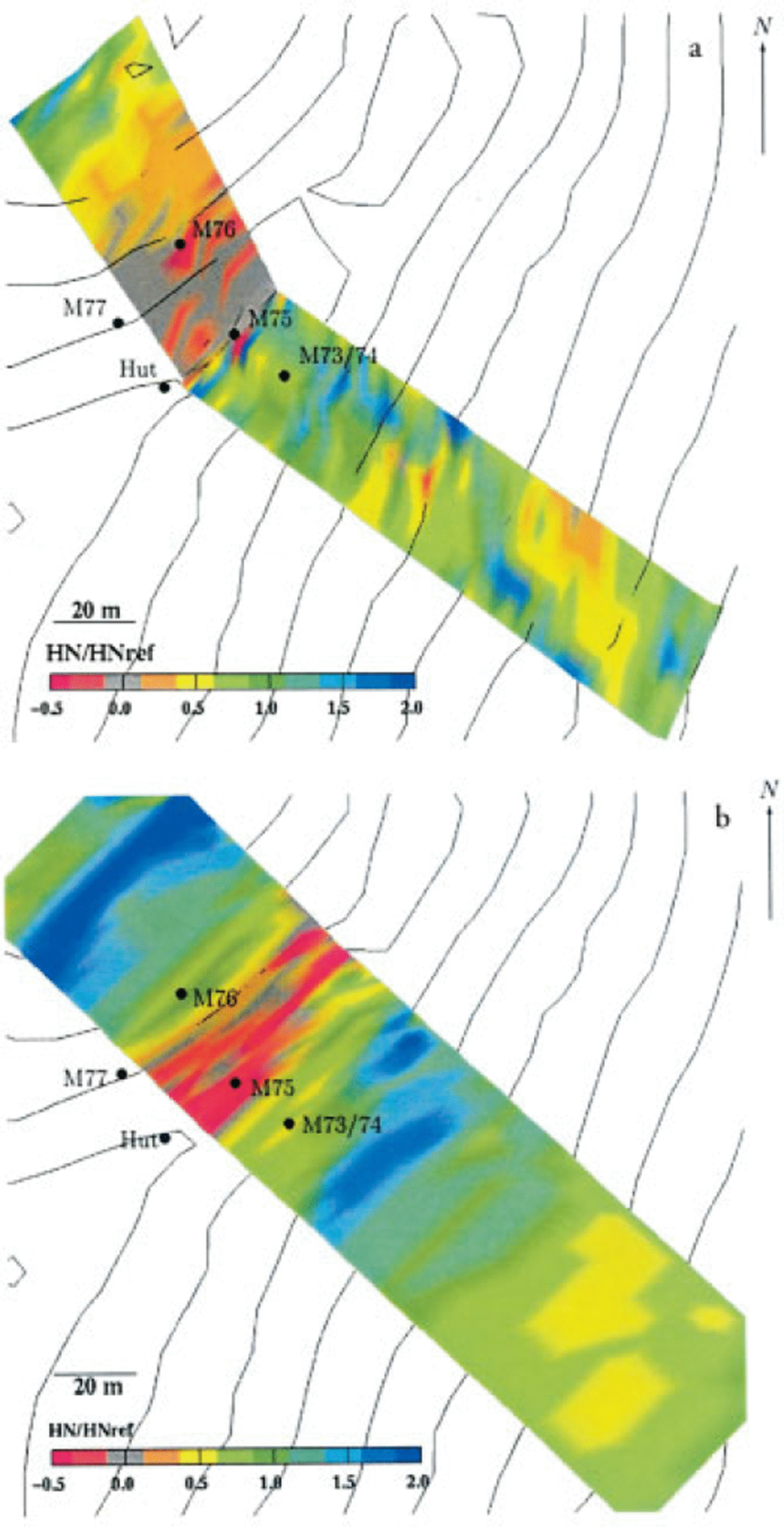
The measurements still show some variability, but also some trends can be discerned: one can see the erosion area in the windward slope near the crest line, the formation of a cornice at the ridge, and an area just leeward of the crest where the snow depth is less than the reference depth. Down-slope areas where HN is twice HN_ref alternate with depletion areas such as the small terrace on the right. It should be recognized that the small-scale terrain features can cause large differences in the erosion and deposition patterns. The simulation does not show the same variability, but nevertheless reproduces some characteristic features such as the windward erosion area close to the crest, alternation between depleted areas and areas of enhanced deposition. As well as the uncertainties due to the poorly known snowpack properties (e.g. the critical shear stress), another reason for the discrepancy between the measurements and the simulation can be found in the history of the snowpack evolution. Thus, snowdrift tends to fill in hollows and to even out the topography in the course of a winter until an equilibrium level of the snow surface is reached where erosion balances deposition. This phenomenon could explain the discrepancy in the depression throughout the windward slope, particularly if the initially measured snow depth at this location was already close to its equilibrium level, whereas for the simulation a uniform initial snow depth was assumed. Thus the simulation might tend to deposit more snow as expected until the equilibrium level is reached. Nevertheless, the results of the simulation give reasonable images.

Another kind of comparison is shown in Figure 12b, which depicts the measured temporal evolution of the new snow at points M77 and M74/73 (windward and leeward of the crest; both masts were equipped with ultrasonic snow-depth sensors) during a drift episode, and the corresponding simulation. This comparison shows that, despite the rough estimates of the snowpack properties, the model can reproduce the temporal evolution of the snow depth quite well. Figure 12a depicts the corresponding wind speed at the top of the crest, and the precipitation rate.

Fig. 12.

(a) Wind speed, M(z = 6 m)(30 min averages), at the top of the crest (M75) and the precipitation rate, RS (10 min sum); wind direction, dd ≈ 315° (northwest), (b) Temporal evolution of the normalized new-snow depth at the points M77 (windward) and M74 (leeward). (Lines denote simulation and markers are measurements.)

Finally, Figure 13 depicts an example of the simulated redistribution pattern of the new-snow layer for the whole simulated area. The new snow is picked up in acceleration regions such as the area close to the crest line, and at small humps and brows. At the crest line, erosion of the old snow-pack is observed as well. Deposition occurs in the deceleration regions leeward of the saddle, in small gullies and in hollows. In this simulation, depositions twice the reference height and erosion depth of about 0.1 m of the old snowpack are found at the crest line. The simulation gives a reasonable image of the redistribution pattern, which tallies with the observations in the field (see, e.g., Fig. 14).

Fig. 13.

Simulated snow distribution. The snow depth is normalized by the reference new-snow depth; negative values indicate erosion of the old snowpack. (HN_ref = 0.48 m; after t ≈ 70 h.) The arrows indicate the simulated wind field fora typical situation approximately 2 m above ground.

Fig. 14.

Slab avalanche at Gaudergrat. The photo was taken on 21 February 1997 after a precipitation period with snowdrift. It shows the saddle and the gully visible in Figure 13, northeast of experimental site.

4. Concluding Remarks

The present model is a step toward accurate numerical simulation of blowing and drifting snow in Alpine terrain. The primary emphasis was on a physically based description of snowdrift suitable for complex Alpine terrain. The model includes: a fully three-dimensional non-steady-state modeling; the modeling of the two main transport modes (saltation and suspension); the dynamical modeling of deposition and erosion, distinguishing between aerodynamic entrainment and ejecta due to particle impacts; the back-reaction of the particles in saltation on the flow (two-way coupling); and the adaptation of the grid to changing snow heights. The comparison between simulations and field measurements is encouraging and indicates that numerical simulations of snowdrift may develop into a powerful tool for land-use planning and avalanche forecasting.

On the other hand, the first numerical simulations also demonstrate the problems with models involving complex terrain. For example, the grid resolution must match the length scale of the terrain. In an early simulation, the simulated wind field differed significantly from the measurements, and the 25 m resolution of the available digital terrain model of the Gaudergrat experimental site proved to be insufficient to resolve key topographic features, like the sharp crest line, in a reasonable way. Special effort had been undertaken to improve the terrain model and thus the numerical grid in the region of interest close to the crest line. A critical point in wind-transport simulation is the non-linear increase of the computational effort with increase of the area of interest and/or spatial resolution of the area. At that point, a compromise must be made between a high spatial resolution and an acceptable computational effort.

Poorly known boundary conditions are a common problem for wind-field simulations in Alpine terrain. To overcome this problem, one might consider using the output of a mesoscale weather model. Some of these models are under development, but are not yet fully adapted for use in mountain areas.

How mechanical properties of the snowpack affect snowdrift rates is still unknown. It is reasonable to expect parameters like erodibility, the rebound probability of particles, the energy loss during impact, the rebound angle, etc., to differ for different snow types, but no systematic investigation has been carried out to study these relationships as yet. The present parameterization of erosion and deposition used in the model is mainly based on wind-tunnel studies and numerical simulations for aeolian particle transport. However, it is possible to include the dependency on varying mechanical snow-pack properties into the model. For that, some research will be necessary to determine these mechanical properties for the varying conditions occurring in nature. This research should include cold-room wind-tunnel studies, similar to those done for aeolian particle transport, using different snow types.

Another still poorly known process is the mutual influence between particle transport and turbulence structure of the airflow within the boundary layer (surface layer) (e.g. the modification of saltation, transition to suspension, or damping of the turbulence). To this end, it would be of interest to do instantaneous profile measurements of the mass flux and the wind speed close to the surface with high temporal resolutions. With improving sensor technology this becomes more and more possible.