INTRODUCTION
Tree rings are a precious archive of the history of our planet in the last millennia, and their study has provided much information of importance to the earth sciences for many years: the cosmogenic radioisotope 14C (radiocarbon) carries information on cosmic-ray variability caused by solar activity (Beer et al. Reference Beer, McCracken and von Steiger2012; Usoskin Reference Usoskin2017). In the last decades, the feasibility of annually resolved 14C measurements in long growth ring sequences has extended the investigation domain to and potentially even beyond the heliosphere. Several rapid increases in the trend of the 14C/12C isotopic ratio vs. ring growth year have been observed (Büntgen et al. Reference Büntgen2018), which provided information about short-term variations of the 14C production rate, and are ascribed to an extraterrestrial origin. In particular two events, occurred in 774 and 993 CE, have been recorded (Miyake et al. Reference Miyake, Nagaya, Masuda and Nakamura2012, Reference Miyake, Masuda and Nakamura2013) originally in Japanese cedar trees, and later in different trees at several latitudes and elevations, as well as in data on 10Be and 36Cl in various ice cores (Mekhaldi et al. Reference Mekhaldi, Muscheler, Adolphi, Aldahan, Beer, McConnell, Possnert, Sigl, Svensson, Synal, Welten and Woodruff2015), revealing the global nature of the events. These events were characterized by an abrupt increase in the measured 14C abundance, expressed as fraction of modern carbon
 $${{\rm{F}}^{14}}{\rm{C}} = \left[ {{{\left( {^{14}{\rm{C}}{/^{12}}{\rm{C}}} \right)}_{{\rm{S}}[-25]}}/{{\left( {^{14}{\rm{C}}{/^{12}}{\rm{C}}} \right)}_{1950[-25]}}} \right]$$
where (14C/12C)S(-25) is the measured isotopic ratio for the sample, blank corrected and adjusted to δ13C = –25‰ and (14C/12C)1950(–25) is the measured ratio of the standard, blank corrected and adjusted to δ13C = –25‰ and recalculated to 1950 CE (Donahue et al. Reference Donahue, Linik and Jull1990).
The observed increase, which is weakly dependent upon latitude (Uusitalo et al. Reference Uusitalo2018), is followed by a slow decline in a few tens of years. Other records regarding different events (Miyake et al. Reference Miyake2017) show a slower rise with time. The different rise and fall time scales can be related to atmospheric circulation mixing and to the biogeochemical cycle. A detailed analysis of the timing of the 774 CE event is reported in Uusitalo et al. (Reference Uusitalo2018) and Güttler et al. (Reference Güttler2015). The present paradigm (Usoskin et al. Reference Usoskin2013; Mekhaldi et al. Reference Mekhaldi, Muscheler, Adolphi, Aldahan, Beer, McConnell, Possnert, Sigl, Svensson, Synal, Welten and Woodruff2015; Sukhodolov et al. 2017; Uusitalo et al. Reference Uusitalo2018) is that both 774 CE and 993 CE events were caused by extreme Solar Proton Events (SPEs). Another event of solar origin was found to occur around 660 BCE (Park et al. Reference Park, Southon, Fahrni, Creasman and Mewaldt2017; O’Hare et al. Reference O’Hare, Mekhaldi, Adolphi, Raisbeck, Aldahan, Anderberg, Beer, Christl, Fahrni, Synal, Park, Possnert, Southon, Bard, Team and Muscheler2019), which appears similar to that of 993 CE. One more event was reported in Wang et al. (Reference Wang, Yu, Zou, Dai and Cheng2017) in 3372–3371 BCE. A further rapid change of over 20‰ is observed in a tree-ring sequence at 5480 BCE (Miyake et al. Reference Miyake2017), which may be a combination of solar proton events with the onset of a solar minimum. Further, Jull et al. (Reference Jull, Panyushkina, Miyake and Masuda2018) observed a similar increase (of ~14‰) over a period about 814–802 BCE, which appears at the onset of a grand solar minimum.
For all the rapid events discussed, a supernova explosion (SN) or a gamma-ray burst (GRB) origin have also been considered and excluded on the basis of the estimated increase of the production rate and the required increase in cosmic ray (CR) flux, although some models have proposed these alternatives (Hambaryan and Neuhäuser Reference Hambaryan and Neuhäuser2013). However, these events did not correspond to known supernova events, so our question here is to investigate 14C over the period of a known SN event. Stephenson and Green (Reference Stephenson and Green2003) documented five historically observed supernovae in 1006, 1054, 1181, 1572 and 1604 CE. Stephenson (Reference Stephenson2015) also reviewed many astronomical phenomena from Chinese records. Damon et al. (Reference Damon, Kaimei, Kocharov, Mikheeva and Peristykh1995) had estimated an upper limit of 6‰ 14C for a large event (close to 1050 ergs) at similar distances (few kpc), based on earlier estimates going back to Lingenfelter and Ramaty (Reference Lingenfelter, Ramaty and Olsson1970). However, it was later shown by Menjo et al. (Reference Menjo, Miyahara, Kuwana, Masuda, Muraki and Nakamura2005) that these variations could be explained by the Schwabe cycle. A systematic investigation on possible 14C spikes in tree rings in the time period corresponding to several historical astronomical records of SN explosions was reported by Dee et al. (Reference Dee, Pope, Miles, Manning and Miyake2016), concluding that no evidence for increase in 14C concentration for any of the 6 examined cases, including SN1054, was found, although there is a small increase at that time in their record. Güttler et al. (Reference Güttler, Wacker, Kromer, Friedrich and Synal2013) proposed that the oscillations observed between 1010 and 1110 CE in biannual measurements on oak tree rings from south Germany can be explained by the 11-year Schwabe solar cycle.
In this work, we present new annually and sub-annually resolved data for the period 1030–1080 CE with the aim to highlight possible anomalies which could be ascribed to the Crab Nebula supernova (SN1054) explosion, which took place in 1054 CE July 4th (Mayall Reference Mayall1939), during the Oort minimum of solar activity (Usoskin Reference Usoskin2017). In order to investigate the possible latitude dependence of the proposed effect, we used an Arctic pine from northeastern Finnish Lapland (68°31′N and 28°09′E, 191 m above sea level) and a mid-latitude sequoia from the Sierra Nevada Mountains, California (36°56′N and 118°75′W, 1890 m asl). We also compare our data with mid-latitude oak data from Germany published by Guttler et al. (Reference Güttler, Wacker, Kromer, Friedrich and Synal2013).
Theoretically, a notable increase of 14C production could be associated with γ-ray emission from a GRB or a SN explosion (Pavlov et al. Reference Pavlov2013). Contribution from charged CR particles in a case of GRB or a distant SN is not expected. The CR signal from SN1054 (~2 kpc distance) would be strongly attenuated and delayed by about a million years due to diffusive transport of charged particles scattered due to inhomogeneities of the galactic magnetic field (Berezinskii et al. Reference Berezinskii, Bulanov, Dogiel, Ginzburg and Ptuskin1990). A very conservative estimate yields that an F14C increase of a few permil would require about 1051 erg released by the SN in photons with energy >10 MeV, assuming an isotropic flux. Since typically <1% of the total energy of a SN explosion is released as hard emission (Hambaryan and Neuhäuser Reference Hambaryan and Neuhäuser2013), this would lead to roughly 1053 erg of the total SN explosion, which is several orders of magnitude greater than kinematic estimates of ~1050 erg (Yang and Chevalier Reference Yang and Chevalier2015). Thus, if a statistically significant increase in F14C is observed in 1054 CE, the standard SN model cannot explain it and would eventually need to be revisited. It should be mentioned that an unambiguous marker of non-SN origin of a 14C enhancement would be the presence of a simultaneous significant and hemispherically symmetric increase of 10Be: γ-rays may produce 14C but not 10Be in the Earth’s atmosphere (Pavlov et al. Reference Pavlov2013). Accordingly, a radiocarbon signal alone is not sufficient to conclude on possible GRB origin of any enhancement and only a multiproxy analysis can make the ultimate assessment.
MATERIALS AND METHODS
Sampling and Sample Treatment
The pine (Pinus sylvestris) set of tree rings was sampled from a subfossil tree trunk unearthed during the fieldwork by scuba diving in the sediment of Lake Kompsiojärvi, in northeastern Finnish Lapland. The tree trunk was pulled to the shore, the sample disk was sawn and the trunk was returned to the lake. Tree-ring widths were measured in the tree-ring laboratory of Natural Resources Institute Finland, to the nearest 0.01 mm and the resulting series was cross-dated statistically and visually against the existing master chronology (Eronen et al. Reference Eronen, Zetterberg, Briffa, Lindholm, Meriläinen and Timonen2002; Helama et al. Reference Helama2008). The rings of this sample represent the 996–1236 CE period. The whole-wood ring separation for the interval 1031 CE through 1080 CE was done using surgical blades under microscope. The wood slivers were processed to α-cellulose (Helama et al. Reference Helama2015), featuring multiple glass funnels connected via custom-built PTFE drainage blocks. The process consists of two alkaline extractions (NaOH), with chlorination step (NaClO2) in between. The resulting α-cellulose was homogenized using an ultrasonic probe (Laumer et al. Reference Laumer2009) and freeze-dried.
The Sequoia set of tree rings was subsampled for earlywood and latewood sections for the interval 1037–1067 CE. We used the giant sequoia specimen CMC-6f (Sequoiadendron giganteum [Lindl.] Buchholz) archived at the Laboratory of Tree-Ring Research (LTRR), University of Arizona. The sequoia specimen was collected in the 1980s at the Circle Meadow Center site located on the western slope of south-central part of the Sierra Nevada Mountains in the King Canyon National Park, California. The calendar age of the rings was established with cross-dating of the CMC-6f ring-width series against the regional giant sequoia tree-ring chronology from the central Sierra Nevada (Brown et al. Reference Brown, Hughes, Baisan, Swetnam and Caprio1992). The tree-ring widths were measured on a LINTAB measuring stage at 0.01 mm precision. The early and latewood of rings were separated with a razor blade under a microscope, and the wood samples were ground. Each powdered wood sample was converted to holocellulose using standard procedures at the Isotope Climatology and Environmental Research Centre (ICER) in Debrecen, Hungary (Molnar et al. Reference Molnar2013).
Radiocarbon Measurements
Cellulose samples were combusted to CO2 and converted to graphite and 14C/12C isotopic ratio measurements on both tree-ring sequences (1031–1080 CE for the Arctic pine and 1038–1068 CE for the sequoia) were measured at the CIRCE (Terrasi et al. Reference Terrasi2008) and the ICER (Molnar et al. Reference Molnar2013) AMS facilities. The α-cellulose samples from the pine were independently graphitized at CIRCE and ICER, using the respective protocols at the two laboratories (Marzaioli et al. Reference Marzaioli2008; Molnar et al. Reference Molnar2013) and separately measured at both facilities. The same procedure was adopted for the late wood (LW) samples from the sequoia, while the early wood (EW) samples were graphitized and measured only at ICER.
The CIRCE isotopic ratio measurements were performed at 2.55 MV terminal voltage at the tandem accelerator Pelletron 9SDH-2 in Caserta. IAEA C3 standard samples were used for normalization, and OXII and C2 for consistency checks. F14C values were obtained after background correction, using processed Aesar graphite, and fractionation correction, using on-line δ13C measurements; finally, Δ14C values (in permil) were extracted using the known ring ages:
 $${\Delta ^{14}}{\rm{C}} = \left[ {{{\rm{F}}^{14}}{\rm{C}} \cdot {\rm{exp}}\left( {{\rm{y}}/8267} \right)-\!\!1} \right] \cdot 1000$$
with y equal to the calibrated age of the sample in years BP. Typical 1σ uncertainty was ∼3‰.
Radiocarbon dating was performed at ICER using the 200 kV MICADAS at the Institute of Nuclear Research in Debrecen, Hungary (Molnar et al. Reference Molnar2013). The measurements were compared to NIST oxalic-II standards (SRM-4990C) and IAEA C-1 for a process blank, and on-line δ13C measurements for correction of isotopic fractionation. 14C calculations and data reduction were done using standard BATS software (Wacker et al. Reference Wacker, Christl and Synal2010).
Wavelet Analysis
In order to verify if our observations can be explained by assuming a contribution to 14C production arising from the radiation flux originated from SN1054 we undertook a detailed analysis of the various frequency components. We first performed a discrete Fourier transform (DFT) analysis on both the pine and the sequoia data sets. The frequency spectra did not show any significant peak: this was attributed to the limited investigated range. Then, we applied the Matlab code for a continuous wavelet transform (CWT) analysis using the analytic wavelet Morlet (Gabor), for which the analyzed signals were the values of 1+Δ14C/1000 vs. ring growth year of the three trees.
In detail, for each of the 3 temporal series a CWT analysis was applied for 5000 times onto a randomly chosen Monte-Carlo dataset produced by hypothesizing normally distributed measurement variables with standard deviations equal to the corresponding experimental uncertainty. CWT, based onto the data set dimension, automatically defines the frequency (and period) scale of analysis. Produced CWT complex coefficients matrices were averaged, and their standard deviations estimated. Average energies were estimated for each produced Monte-Carlo dataset. Monte-Carlo associated uncertainties attributable to experimental errors were also estimated and utilized in order to infer zones of significance of the produced scalograms. A statistic defined as the ratio between the energy of the average wavelet and its associated error was evaluated and contour plots produced with a significance higher than 2σ (i.e. 2, 2.5 and 3) were superimposed on the previously produced scalograms and scaled at the Sequoia time and period frame to improve comparison among datasets.
RESULTS
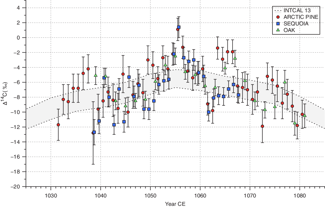
The results obtained at the two laboratories are reported in the Appendix, showing a good agreement between the results of the measurements performed in the two laboratories. The resulting weighted averages for Δ14C data are presented in Figure 1 for the pine and the sequoia. For comparison the IntCal13 calibration curve (Reimer et al. Reference Reimer, Bard, Bayliss, Beck, Blackwell, Bronk Ramsey, Buck, Cheng, Edwards, Friedrich, Grootes, Guilderson, Haflidason, Hajdas, Hatté, Heaton, Hoffmann, Hogg, Hughen, Kaiser, Kromer, Manning, Niu, Reimer, Richards, Scott, Southon, Staff, Turney and van der Plicht2013) is also shown: taking into account that in the investigated range all IntCal13 raw data are decadal averages (except 1 point at 1047 CE) it can be observed that the average behavior is well reproduced by our data. This indicates that we do not observe the 25–40-year offset reported previously in Güttler et al. (Reference Güttler, Wacker, Kromer, Friedrich and Synal2013). The annual resolution allows us to highlight a Δ14C increase around 1055 CE with similar shapes at both latitudes: if we exclude the data points between 1054.5 and 1056.5 the average value in the interval 1050–1060 is –5‰ (on both sides of the peak) to be compared with the maximum of +1‰, to be compared with a value of ∼12‰ observed for the Miyake events. Taking into account that the average uncertainty of the weighted averages is ∼2‰, the observed increment is at ∼3σ level. The rise time is quite sharp (with a possible first increase in 1054 CE), while, in contrast to the Miyake events in 774 and 993, the decay time is only slightly larger than the rise time. Moreover, a second stepwise increase of comparable intensity and a slower decline is observed 8 years after the first one (in 1063) only for the Arctic pine, with an increment of ∼7‰, while no statistically significant (larger than 1σ) increase is observed for the sequoia. We have plotted in Figure 1 also the data from Güttler et al. (Reference Güttler, Wacker, Kromer, Friedrich and Synal2013), which correspond to an intermediate latitude (note the biannual resolution of the latter series). In order to take into account the offset reported by the authors, we have added to their data a bias of 4‰. The data points in 1055 show a local maximum similar to the pine and sequoia data, even if attenuated as an effect of the biannual averaging. Data points in the 1063–1067 AD range lie between the pine and sequoia series. It is not clear if this may reflect a latitudinal trend: actually, all oak data points (with the exception of the latter) differ by less than 1σ from the averages of pine and sequoia data corresponding to the two years covered.
Weighted averages of the two single-year measurement series for the sequoia tree rings (blue squares) and the Arctic pine (red dots). Biannual 14C data from Güttler et al. (Reference Güttler, Wacker, Kromer, Friedrich and Synal2013) derived from German oak tree rings are shown with green triangles. The latter series is adjusted with a 4‰ offset reported by the authors. (Please see electronic version for color figures.)

DISCUSSION AND CONCLUSIONS
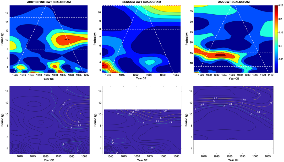
The data immediately preceding or following the quoted increments show an oscillatory behavior with a pseudo period of about 10 years, superimposed on an overall trend resembling the positive lobe of a slower trend, with a half-period of about 100 years. Both oscillations suggest the influence of solar cycle components, which could eventually modify the shape of a possible signal associated to SN1054. Application of the CWT analysis to each of the three data sets produced the scalograms shown in Figure 2, allowing the detection of the most representative scales (or frequencies) of the signals. The cones of influence drawn indicate the regions in the growth year–period plane where edge effects of the CWT become significant. The wavelet results show similar frequencies of the 14C variability for both time series: both the well pronounced variability with the period of about 8–14 years (Schwabe cycle, cut for the sequoia because of the limited time range), and the moderately high signal in the period range between 4 and 6 years, caused by the peak in 1055 CE, can be observed. In the pine data set, this peak with the 4–6-year period is followed by a second peak about 7 years later producing a 2σ area of significance. These frequency features, with the exception of the 4–6 periodicity are also seen in the oak data, though not so strongly as in the sequoia and pine series probably due to biennial averaging.
Upper panels: scalograms of the three discussed time series. The iso-contour levels on the right represent the normalized percentage of power for each period in the studied time series, i.e. the contribution of the oscillation with a given frequency to the data of a single year. The cone of influence (dashed white line) separates the regions that may be affected by edge effects from the significant CWT areas. Lower panels: contour lines of the significance parameter for the scalogram points defined as the inverse of the relative standard deviation. Note the different scales on both axes in the upper panels, due to the different ranges investigated; in order to facilitate the comparison among the three cases, the figures in the lower panels were cut so to represent the same portion of the growth year–period plane.

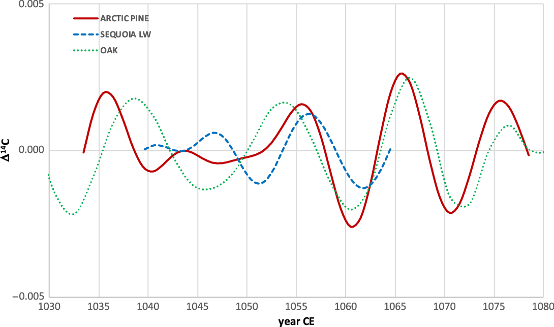
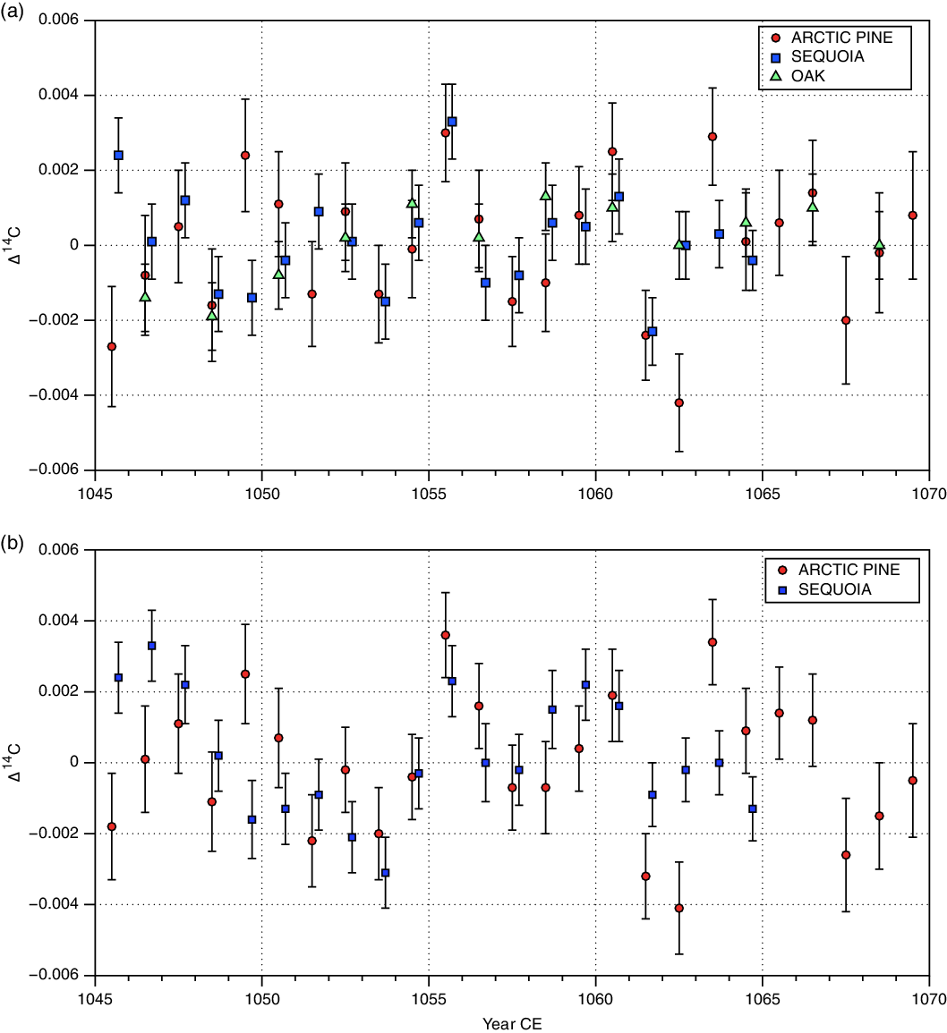
In conclusion, we found clear oscillations with period around 11 years during 1050–1063 CE. The 1055 CE peaks match each other in the sequoia and pine data and occur after the 1054 CE impact year. If we assume that the observed 11-year oscillation is due to the solar activity, then the 1055 CE peak appears during the solar minimum. Furthermore, we estimated the net signal isolated after subtraction of the underlying solar cycle contribution in two ways: firstly, for each data set, the baseline contribution was evaluated subtracting from the respective experimental data all the wavelet frequency components and smoothing the result by a running 5-year average; then, the 11-year cycle contribution was modeled by scaling with the 8–15-year window (8–10.8 for the sequoia series):this window is indicated in Figure 2 (upper panel) and corresponds to the period interval in which all three scalograms show the maxima of the above defined significance parameter. The corresponding reconstructed signals are shown in Figure 3. Finally, the net signals were deduced by subtraction of the estimated background from the experimental data: the result is shown in Figure 4a. One can see that the signal is localized to a single-year increase in Δ14C at the level of 3–4‰, which may have different possible origins, such as the SN, unusually weak solar cycle minimum, or even a SEP event, but the latter is unlikely considering the shape of the event. A local anomaly of the carbon cycle is unlikely either because of the synchronization of the signals in very different locations. Secondly, we estimated the net signal of the pine and sequoia data with more robust (longer time interval) oak background: the shortness of the sequoia time series may have distorted the estimated solar cycle contribution. Within the experimental uncertainties, the net signal remains unchanged (Figure 4b) and shows an excursion in 1055 CE of the order of 4‰ in the 1+Δ14C/1000 behavior. This excursion, even if the corresponding step has only a ∼2σ height, is observed at the same location and intensity in the pine and sequoia data sets, while it is probably attenuated by the biannual sampling in the oak data, indicating the global nature of this possible event.
Wavelet reconstruction of the signal representing the 11-year cycle contribution to the 14C intensity obtained through conditioning the scalogram scale values over the 8–15-year band.

Net signal after subtraction of the solar cycle contribution (Figure 3) from the experimental data (Figure 1): (a) subtraction result from each time series as estimated by the wavelet analysis of relevant tree-ring series; (b) subtraction result from each time series as estimated by the more robust wavelet analysis of the long oak data set.

The shape of this peak is quite different from previously determined abrupt 14C excursions (e.g. 774 CE, 994 CE and 660 BCE) and suggests a different origin. The absence of a slow setting following the initial offset is hardly reconcilable with the atmospheric mixing. It has to be noted that, in the eventuality of a γ-ray origin of 14C production, it would enter significantly also to troposphere and rise and fall times would be probably faster since stratospheric residence time would not play a role, as indicated by preliminary carbon-cycle calculations. Moreover, whether the presence of a sharp peak without slow decay is a real effect or it is caused by an incorrect deconvolution of the underlying background requires a detailed modeling which is beyond the aim of the present work and will be addressed in a forthcoming paper. This possibility is suggested by the fact that the F14C values in the range 1058–1067 CE are slightly larger than the average background, even if with a low statistical significance. A multiproxy data analysis, including annually resolved records of 10Be in polar ice, is required to provide more insight into the origin of this event.
ACKNOWLEDGMENTS
The work of S. Helama, M. Oinonen, P. Nöjd and J. Uusitalo was supported by the Academy of Finland (grants 288083 and 288267). Work by G. Kovaltsov, S. Poluianov and I. Usoskin was partially supported by the Academy of Finland (Project ESPERA 321882). A.J.T. Jull, M. Molnar and T. Varga acknowledge partial support by the European Union and the State of Hungary, co-financed by the European Regional Development Fund in the project GINOP-2.3.2.-15-2016-00009 “ICER”. All data are available in the Appendix.
APPENDIX
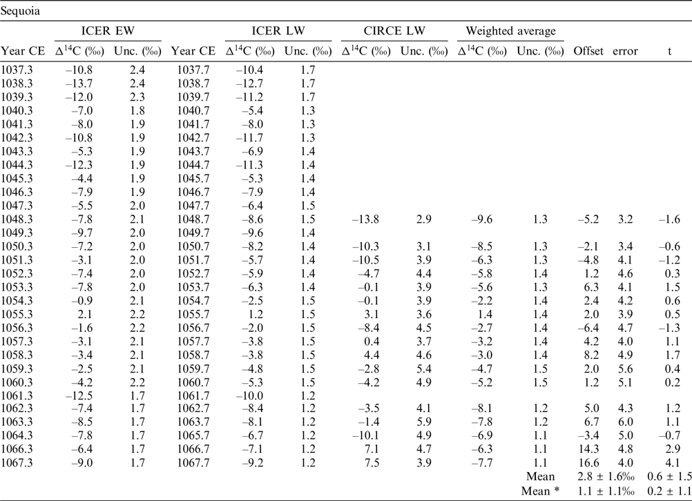
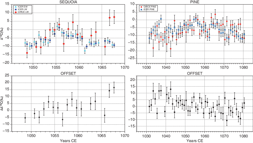
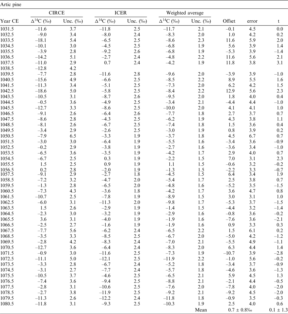
Measured values of annually resolved Δ14C are reported in Table A1 and in Figure A1 a) and c) for the sequoia tree rings and in Table A2 and in Figure A1 b) and d) for the arctic pine. In order to take into account the different growing seasons of the (portion of) rings, we adopted the following convention for the horizontal axis: the EW data were referred to by the integer year plus 0.3; for the LW we added 0.7 years and 0.5 years for the bulk. The vertical bars are 1σ uncertainties. The plot in panel a) includes the EW data, which were measured only in Debrecen. In panels c) and d) the relative offsets between the two data sets are displayed with the propagated uncertainty: for each pair of values measured in both laboratories Δ14CC(I) ± σC(I) (with subscripts C and I for CIRCE and ICER respectively) the difference between them was calculated with the propagated error and the t variable, defined as:
 $$t = ({\Delta ^{14}}{{\rm{C}}_{\rm{C}}} - {\Delta ^{14}}{{\rm{C}}_{\rm{I}}}){\rm{/}}{({\sigma _{\rm{C}}}^2 + {\sigma _{\rm{I}}}^2)^{1/2}}$$
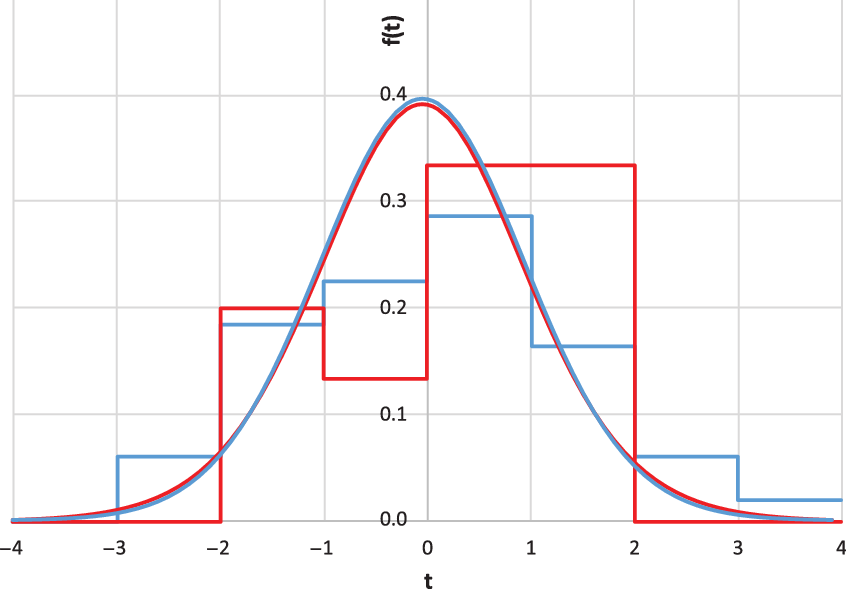
was calculated. With the exception of the last two values in Table A1, all offsets are well within the ± 3σ range, indicating a good agreement between the two data sets. The distributions of the t-values have average values of 0.1‰ and 0.6‰ and standard deviations of 1.1‰ and 1.5‰, for the pine and the sequoia, respectively (0.2 ± 0.1‰ for the sequoia excluding the two outliers). The t mean values and standard deviations were found to be 0.2 ± 1.1 and 0.1 ± 1.3, respectively, in good agreement with the expected values. The histograms of t variables are compared in Figure A2 with the corresponding Student’s-t distributions with 13 and 47 degrees of freedom, respectively. The Pearson χ2 values are 4.1 and 2.9 with 7 degrees of freedom for the sequoia and the pine data, respectively, to be compared with a 5% confidence limit of 14. Finally, the weighted averages:
 $${\rm{w}}.{\rm{a}}. = ({\Delta ^{14}}{{\rm{C}}_{\rm{C}}}{\rm{/}}{\sigma _C}^2 + {\Delta ^{14}}{{\rm{C}}_{\rm{I}}}{\rm{/}}{\sigma _{\rm{I}}}^2){\rm{/}}(1{\rm{/}}{\sigma _{\rm{C}}}^2 + 1/{\sigma _{\rm{I}}}^{\rm{2}});\quad {\sigma _{{\rm{wa}}}}{\rm{ = }}1{\rm{/}}{(1{\rm{/}}{\sigma _{\rm{C}}}^2 + 1/{\sigma _I}^2)^{1/2}}$$
were calculated and are reported in the tables. Due to the large uncertainty of the two outliers, their inclusion does not affect the final result significantly.
Results of the ICER measurements of single year Δ14C for the sequoia earlywood, and of the CIRCE and ICER measurements for the sequoia latewood. Weighted averages and differences between the pairs of values for the latter are also reported. The last column represents the Student’s-t variable values.

Interlaboratory comparison of the Δ14C values measured for the earlywood and latewood sequoia (upper left) and for the Arctic pine (upper right) at CIRCE and ICER. Lower panels show the differences between the two series with the propagated errors. The time scale of early/late wood measurements is adjusted to the total ring width measurements of other series.

Results of the CIRCE and ICER measurements of single year Δ14C for the arctic pine tree rings. Weighted averages and differences between the pairs of values are also reported with their errors. The last column represents the Student’s-t variable values.

Histogram of relative offsets between the CIRCE and ICER measurements of Δ14C for the sequoia (blue) and arctic pine (red) tree rings compared with the Student’s-t distributions with 13 and 47 d.o.f, respectively.