


1. Introduction
The Taylor–Couette flow of a viscous incompressible fluid between two coaxial cylinders that are infinitely long is a paradigm for studies of stability and transition to turbulence. A survey of the literature on the Taylor–Couette problem can be found in Koschmieder (Reference Koschmieder1993) and Tagg (Reference Tagg1994). In the usual case, the inner cylinder of radius  $R_1$ is rotating with angular velocity
 $\varOmega _1$ and the outer cylinder of radius
 $R_2$ is stationary. The radius ratio will be denoted
 \begin{equation} \eta=R_1/R_2 <1. \end{equation}
The axial length  $\ell$ is, in most implementations, much larger than the gap,
 \begin{equation} d=R_2-R_1, \end{equation}
i.e. the aspect ratio
 \begin{equation} L=\ell/d \end{equation}
is much larger than 1 ( $L \gg 1$). In the basic state, commonly called circular Couette flow (CCF), only the azimuthal velocity
 $u_\theta$,
 $\theta$ standing for the azimuthal angle, is non-zero and it is a decreasing function of only the radius
 $r$.
1.1. TVF in Newtonian fluids
As demonstrated by Taylor (Reference Taylor1923), as inertial effects start to dominate over viscous ones, CCF becomes unstable giving rise to the TVF characterized by stationary counter-rotating vortices stacked along the axial direction. The onset of instability can be parameterized by the Reynolds number (1.5). Equivalently, the Reynolds number can be used. In most common configurations the outer cylinder is at rest and the inner one rotates with angular velocity  $\varOmega _1$. This defines the velocity scale
 \begin{equation} U_{ref}=R_1 \varOmega_1. \end{equation}
In an incompressible Newtonian flow with uniform viscosity  $\mu$ and density
 $\rho$ where kinematic viscosity
 $\nu =\mu /\rho$ is well defined, the standard definition of the Reynolds number using the gap
 $d$ as length scale results in
 \begin{equation} {Re}= R_1 \varOmega_1 d /\nu. \end{equation}
The critical Reynolds number of the onset of TVF will be denoted  $Re_c$. The canonical configuration, most convenient for theoretical study, consists in considering a small gap
 $\eta \rightarrow 1$ and an infinite aspect ratio
 $L \rightarrow \infty$ (Taylor Reference Taylor1923). However, in practical cases, in particular, experimental implementations, large gaps and finite aspect ratios occur. The values of the critical Reynolds for several values of the radius ratio are available in the literature (see for instance table 1 in DiPrima, Eagles & Ng (Reference DiPrima, Eagles and Ng1984)). Approximate expressions of
 ${Re}_c(\eta )$ can be found in Esser & Grossmann (Reference Esser and Grossmann1996) and Dutcher & Muller (Reference Dutcher and Muller2007). Concerning the influence of the aspect ratio, Cole (Reference Cole1976) has shown experimentally that there is practically no effect of the annulus length on the critical Reynolds number for an aspect ratio
 $L$ as low as
 $8$. The interaction between the endwall boundary layer and the centrifugal Taylor instability has been studied numerically by Czarny et al. (Reference Czarny, Serre, Bontoux and Lueptow2003) for a particularly low value of aspect ratio
 $L = 6$.
1.2. Stability of Taylor vortices in Newtonian fluids
For small gap width, the range of Reynolds number  $Re$, in which the axisymmetric vortices remain stable is small. For instance, in the experiments of Cole (Reference Cole1976) where
 $\eta = 0.95$ and
 $L = 60$, the TVF becomes unstable with respect to azimuthal disturbances at
 $Re_s = 1.05 Re_c$. A bifurcation from TVF to the wavy vortex flow (WVF) is observed. The structure of the WVF and the doubly periodic (axially and in time) motion was first studied experimentally by Coles (Reference Coles1965). Unlike the transition to TVF, the Reynolds number
 $Re_s$ of the onset of the secondary instability yielding WVF depends significantly on the aspect ratio
 $L$. It increases strongly when the aspect ratio
 $L$ is reduced below 40, as has been shown experimentally by Cole (Reference Cole1976). For
 $L \ge 40$, with
 $\eta > 0.89$,
 $Re_s$ changes by only a few per cent. The azimuthal wavenumber varies on a much wider range. It ranges from
 $2$ to
 $8$ depending on the conditions by which the second transition is approached (Coles Reference Coles1965; Cole Reference Cole1976; Mullin Reference Mullin1985; Dutcher & Muller Reference Dutcher and Muller2009). The non-uniqueness of this flow has been also observed through the existence of hysteresis phenomena (Coles Reference Coles1965). In other words, multiple stable flow states could be reached for a given Reynolds number. Concerning the physical mechanisms that drive the transition from TVF to WVF, they were discussed by Martinand, Serre & Lueptow (Reference Martinand, Serre and Lueptow2014) and Dessup et al. (Reference Dessup, Tuckerman, Wesfreid, Barkley and Willis2018).
For  $\eta < 0.75$,
 $Re_s$ increases rapidly as
 $\eta$ decreases Jones (Reference Jones1985). For instance, for
 $\eta = 0.67$,
 $Re_s \approx 5 Re_c$. This tendency is in agreement with the experimental results of Snyder & Lambert (Reference Snyder and Lambert1966), Meincke & Egbers (Reference Meincke and Egbers1999) and King et al. (Reference King, Li, Lee, Swinney and Marcus1984). A recent direct numerical simulation by Razzak, Khoo & Lua (Reference Razzak, Khoo and Lua2019) in a wide gap setup
 $\eta =0.5$ yielded
 $Re_s \approx 8.45 Re_c$. In their study, a four wavelengths fluid column is considered (
 $L = 4 \, \varLambda = 7.944$) with periodic boundary conditions in the axial direction. For this relatively small aspect ratio, Razzak et al. (Reference Razzak, Khoo and Lua2019) evidenced an intermediate step between TVF and WVF in the interval
 $6.2 \, {Re}_c \leq {Re} \leq 8.45 \, {Re}_c$. They found that the flow becomes non-axisymmetric with a strong azimuthal wave in the inflow region (inward oriented flow of the TVF vortex array) as compared with the outflow region. Three decades earlier, the linear stability of the Taylor vortices was investigated by Jones (Reference Jones1985) for the same radius ratio
 $\eta = 0.5$. The axisymmetric solution was determined using a Fourier expansion in the axial direction with a period of one or two axial wavelengths, and a Chebychev polynomials in the radial direction. He found that the results depend on the axial wavelength
 $\varLambda$ selected. For
 $\varLambda < 2$ (
 $1.6$ and
 $1.7$ in the table 1 of his paper), Jones (Reference Jones1985) detected a wavy outflow boundary mode at
 ${Re} \approx 5 \, {Re}_c$. In this mode, the oscillation amplitude is localized in the outflow boundary jet and adjacent outflow boundaries jets oscillate in antiphase, i.e. the flow is axial subharmonic with respect to the period of Taylor vortices. If
 $\varLambda > 2$ a direct transition to WVF is observed. Still earlier, Lorenzen, Pfister & Mullin (Reference Lorenzen, Pfister and Mullin1983) observed experimentally, for
 $\eta$ around
 $0.5$, a transition from TVF to wavy outflow boundary mode when the axial wavelength is less than
 $2$ (the size of one vortex is less that the gap width). In their experiments, the number of vortices was kept constant as
 $L$ is varied so that the size of individual vortices varied.
Hence, for a wide gap,  $\eta$ around 0.5, wavy modes different from the conventional WVF are obtained numerically and experimentally. The type of wavy mode observed is probably very sensitive to the aspect ratio, the size of vortices and may also be very sensitive to the type of boundary conditions. Furthermore, the wavy mode obtained by Razzak et al. (Reference Razzak, Khoo and Lua2019) was not predicted by the linear stability analysis done by Jones (Reference Jones1985). Therefore, we believe that additional experimental or numerical data are needed for a wide gap geometry. Concerning, the effect of endwalls on the WVF, it has been shown numerically by Czarny et al. (Reference Czarny, Serre, Bontoux and Lueptow2004), that this effect does not penetrate far from the endwall. The waviness is already present one or two vortices away from the endwall.
Configurations with finite aspect ratio  $L$ or given axial period lead to restrictions of the axial wavenumber of axisymmetric TVF. At the critical Reynolds number
 ${Re}_c$, the axial wavenumber
 $k$ can have only a single, unique value,
 $k_c$. For
 ${Re} > {Re}_c$, TVF solutions to the equations of motion exist for a range of wavenumbers which depends on the reduced Reynolds number
 $\epsilon =({{Re}-{Re}_c})/{{Re}_c}$ and the boundary conditions. However, the resulting solutions of such a system are not all stable. The stability of these solutions with respect to axisymmetric perturbations is a fundamental mechanism which delimits the width of the stable band of wavenumbers. Close to the marginal stability curve of the Couette flow, the limits of the stable band can be determined using amplitude expansion up to third order (Kogelman & DiPrima Reference Kogelman and DiPrima1970). A first detailed investigation of the stability of TVF solutions with respect to axisymmetric perturbations was done numerically by Riecke & Paap (Reference Riecke and Paap1986) for three radius ratios:
 $\eta = 0.892$;
 $0.75$;
 $0.5$. It was followed by that of Paap & Riecke (Reference Paap and Riecke1990) for
 $\eta = 0.5$ and larger values of
 $\epsilon$. Overall, a stationary TVF solution for a given wavenumber
 $k$ is computed, at different values of
 $\epsilon$, using a Galerkin method with Fourier expansion in the axial direction and Chebyshev polynomials in the radial direction. Using Floquet theory, the linear stability analysis of this solution, with respect to infinitesimal perturbations with wavenumber
 $\tilde {k}$ leads to an eigenvalue problem, the least stable eigenvalue of which is real, i.e. represents the growth-rate
 $\sigma (\tilde {k})$ of a stationary perturbation. A TVF solution with a wavenumber
 $k$ is unstable when the growth rate
 $\sigma (\tilde {k})$ is positive for some value of
 $\tilde {k}$. Two types of instabilities can be distinguished according to the value of
 $\tilde {k}$ for which
 $\sigma (\tilde {k})$ first becomes positive. The first one corresponds to the case where
 $\sigma (\tilde {k})$ first exceeds zero near
 $\tilde {k}=0$, the instability is of Eckhaus type, i.e. of long wavelength (Riecke & Paap Reference Riecke and Paap1986; Paap & Riecke Reference Paap and Riecke1990; Dennin, Cannell & Ahlers Reference Dennin, Cannell and Ahlers1994). In this case, the adjustment of the wavenumber is done by creation of a pair of vortices (if
 $k$ is too low) or pairing of vortices (if
 $k$ is too large) and a new stationary stable state is reached. The second type of instability corresponds to the case where
 $\sigma (\tilde {k})$ first exceeds zero near
 $\tilde {k}=k/2$. It is called short-wavelength instability. In this case, the adjustment of the wavenumber is done by merging every two vortex pairs into a single one (when
 $k$ is too high) or by adding a vortex pair between every two base vortex pairs (when
 $k$ is too low). Riecke & Paap (Reference Riecke and Paap1986) and Paap & Riecke (Reference Paap and Riecke1990) found that the band of stable wavenumbers is mainly delimited from either the low
 $k$- or high
 $k$- side by the Eckhaus instability mechanism. However, for
 $\epsilon > 1$ and from the high
 $k$-side, the stable band is delimited by the short wavelength instability. Excellent agreement exists between the theoretical results of Riecke & Paap (Reference Riecke and Paap1986) and Paap & Riecke (Reference Paap and Riecke1990) and the experimental observations of Dominguez-Lerma, Ahlers & Cannell (Reference Dominguez-Lerma, Ahlers and Cannell1984) and Dennin et al. (Reference Dennin, Cannell and Ahlers1994). Similar theoretical calculations done by Guo & Finlay (Reference Guo and Finlay1991) lead to the same results. Riecke & Paap (Reference Riecke and Paap1986) and Paap & Riecke (Reference Paap and Riecke1990) have noticed that the width of the band of stable wavenumbers is much smaller than that predicted from amplitude expansion. Furthermore, this behaviour is more pronounced with a lowering of the radius ratio. It was also observed theoretically and experimentally that on the low
 $k$-side, the stability limits departs rather suddenly from the amplitude expansion result with increasing
 $\epsilon$. According to Riecke & Paap (Reference Riecke and Paap1986) this structure arises from the interaction of modes with resonating wavenumbers. The first such resonance occurs between
 $k$ and
 $2 \, k$. This point has been discussed by Meyer-Spasche & Keller (Reference Meyer-Spasche and Keller1985).
Note that, for a narrow gap, when  $Re$ is increased further, the WVF bifurcates to modulated WVF characterized by two incommensurate temporal frequencies (Andereck, Liu & Swinney Reference Andereck, Liu and Swinney1986). Shortly after the onset of the second frequency, the flow becomes chaotic or weakly turbulent (Brandstäter et al. Reference Brandstäter, Swift, Swinney, Wolf, Farmer, Jen and Crutchfield1983). This orderly progression of nonlinear states makes the Taylor–Couette flow an attractive model for studying the influence of rheology of non-Newtonian fluids on the instability mechanisms and transition to turbulence.
1.3. Brief review on Taylor–Couette flow of shear-thinning fluids
A common feature of many non-Newtonian fluids is the shear-thinning behaviour, i.e. a nonlinear decrease of the viscosity when the shear rate increases. Polymer and colloid solutions as well as particulate dispersions exhibit this behaviour above a certain concentration threshold. Actually, these fluids are also viscoelastic to varying degrees. Hereafter, we focus on shear-thinning fluids for which the elastic response does not play a significant role. Typically, stiff polymers show significant nonlinear decrease of viscosity with the shear-rate, with almost negligible elastic effect (Lindner, Bonn & Meunier Reference Lindner, Bonn and Meunier2000). The shear-thinning behaviour arises from the reorganization of the internal fluid structure reducing the viscous dissipation. We will assume that the characteristic time of the reorganization of the flow structure is much smaller than all characteristic times of the problem.
Several works have been devoted to the influence of shear-thinning behaviour on threshold of instabilities in Taylor–Couette flow as well as to the features of Taylor vortices.
Circular Couette flow of a shear-thinning fluid is mainly characterized by a viscosity stratification in the annular space, which is more significant the stronger the shear-thinning effects and the wider the annular space. With increasing shear-thinning effects, the shear rate increases at the inner wall and decreases at the outer one. Furthermore, the nonlinear variation of viscosity with the shear rate introduces, at the linear level, an anisotropy of the deviatoric tensor associated with the perturbation.
The mechanism of instability of CCF of shear-thinning fluids with negligible viscoelasticity is the same as for a Newtonian fluid and results in axisymmetric counter-rotating vortices separated by radial inflow and outflow jets emanating from the fluid layers adjacent to the cylinder wall. However, the critical conditions are different because of the radial viscosity stratification and the modification of the azimuthal velocity profile. In the case where the inner cylinder is rotating and the outer one is stationary, the critical Reynolds and axial wavenumbers were determined using linear stability analysis, for power-law and Carreau fluids, for wide and narrow annular spaces, see for instance Alibenyahia et al. (Reference Alibenyahia, Lemaitre, Nouar and Ait-Messaoudene2012), Li & Khayat (Reference Li and Khayat2004), Agbessi et al. (Reference Agbessi, Alibenyahia, Nouar and Choplin2015), Topayev et al. (Reference Topayev, Nouar, Bernardin, Neveu and Bahrani2019) and the references therein. It is shown that the wavelength increases slightly with increasing shear-thinning effects when  $\eta >0.7$ and decreases significantly with increasing shear-thinning effects for a wide gap (
 $\eta < 0.6$). In shear-thinning flows the Newtonian definition (1.5) of the Reynolds number requires an additional specification of the viscosity scale
 $\mu _{ref}$ to replace
 $\nu =\mu _{ref}/\rho$. A frequent choice is
 $\mu _{ref}=\mu _0$, where
 $\mu _0$ is the zero-shear viscosity,
 \begin{equation} {Re}={\rho} \, {\varOmega}_{1} {R}_{1}{d}/{\mu}_{0}. \end{equation}
The critical Reynolds number defined using the zero-shear viscosity decreases with increasing shear-thinning effects. A radically different conclusion may be reached if one uses the inner wall-shear viscosity of the fluid as a viscosity scale. Masuda et al. (Reference Masuda, Horie, Hubacz, Ohta and Ohmura2017) used an average viscosity weighted by the strain-rate squared. They found that the critical Reynolds number defined using this average viscosity is the same as for a Newtonian fluid. However, this result is limited only to a narrow annular space with a radius ratio  $\eta > 0.7$. Recently, Elçiçek & Güzel (Reference Elçiçek and Güzel2020) suggested using an average Reynolds number
 $Re_G$, defined as an average over the annular space of the local Reynolds number calculated using the local velocity and the local viscosity. With this definition, it is observed that the critical Reynolds number increases with increasing shear-thinning effects. The selection of the reference viscosity defining the Reynolds number may be considered to be simply a matter of choice, however, it changes the conclusions concerning the effect of shear thinning.
From an experimental point of view, Sinevic, Kuboi & Nienow (Reference Sinevic, Kuboi and Nienow1986) determined the onset of Taylor vortices based on changes in the scaling relationship between the measured torque exerted on the rotating inner cylinder and  $Re$. The results were obtained for two radius ratios
 $\eta = 0.7$ and
 $0.9$, the rheological behaviour of the used fluids, CMC and Carbopol solutions, were described by the power-law model. Using a Taylor–Couette system with a radius ratio
 $\eta = 0.5$, Escudier, Gouldson & Jones (Reference Escudier, Gouldson and Jones1995) determined the transition from CCF to TVF by focusing on the development of the axial velocity component near the inner wall at a radial position
 $r$ such
 $(R_2 - r)/(R_2 - R_1) = 0.8$. The Reynolds number is defined using the inner wall shear viscosity. The used fluids were a glucose solution as a Newtonian fluid reference, an aqueous solution of xanthan gum
 $1500$ p.p.m. which is shear thinning and a Laponite suspension which is shear-thinning and thixotropic. The radius ratio and the aspect ratio of the Taylor–Couette configuration are
 $\eta = 0.506$ and
 $L = 233$. In their experimental work, the authors focus mainly on the development of Taylor vortices. It is indicated that, for shear-thinning fluids, the onset of Taylor vortices is much more gradual than that for a Newtonian fluid.
Concerning the flow structure in the TVF regime, the theoretical (Alibenyahia et al. Reference Alibenyahia, Lemaitre, Nouar and Ait-Messaoudene2012; Agbessi et al. Reference Agbessi, Alibenyahia, Nouar and Choplin2015; Topayev et al. Reference Topayev, Nouar, Bernardin, Neveu and Bahrani2019) and experimental (Escudier et al. Reference Escudier, Gouldson and Jones1995; Cagney & Balabani Reference Cagney and Balabani2019a,Reference Cagney and Balabanib) results indicate that the flow undergoes a significant change with increasing shear-thinning effects. Indeed it is shown that with increasing shear-thinning effects: (i) for a wide gap, the vortex eye is shifted towards the inner cylinder, because of the viscosity stratification – the viscosity increases from the inner cylinder to the outer one; (ii) the vortices are shifted axially towards the radial outflow boundaries; (iii) this axial shift leads to increasing concentration of the vorticity at these boundaries; (iv) the vorticity in the outflow becomes stronger than the inflow and the extent of the inflow zone increases accordingly; (v) the strength of the vortices becomes weak as compared with the velocity of the inner cylinder. Note that, using a weakly nonlinear analysis, Topayev et al. (Reference Topayev, Nouar, Bernardin, Neveu and Bahrani2019) demonstrated for a large range of rheological parameters that the transition to TVF regime for purely viscous shear-thinning fluids remains supercritical.
1.4. Stability of Taylor vortices in shear-thinning fluids
As far as the stability of the TVF is concerned, the results are sparse. In the experiments of Escudier et al. (Reference Escudier, Gouldson and Jones1995) at  $Re_c < Re < 2.5 \, Re_c$, with
 $\eta = 0.506$, it was noticed for aqueous solutions of xanthan gum at
 $1500$ p.p.m. and for Laponite solution, that the vortices exhibit a slow axial drift. A constant drift velocity of
 $3 - 4\ \mathrm {\mu }\text {m}\ \text {s}^{-1}$ was reported.
In a geometrical configuration with a narrow gap,  $\eta = 0.883$ and
 $L = 12.97$, the transition from TVF to WVF was detected and studied by Cagney & Balabani (Reference Cagney and Balabani2019a) and Cagney & Balabani (Reference Cagney and Balabani2019b) using particle image velocimetry (PIV) and visualization. Their results (table III in Cagney & Balabani Reference Cagney and Balabani2019b) indicate that the transition to WVF occurs at
 ${Re}_s \approx 8 \, {Re}_c$ for a Newtonian fluid and at
 ${Re}_s > 8 \, {Re}_c$ for shear-thinning fluids. However, one can note that for the Newtonian fluid, the value of
 $Re_s$ is much larger than that predicted by Cole (Reference Cole1976) for a similar geometry. Furthermore, Cagney & Balabani (Reference Cagney and Balabani2019b) noticed that the amplitude of the wave varies with the axial position. It may be a consequence of endwalls effects.
In a more recent paper, using xanthan gum solutions in a mixture glycerol–water ( $25\,\%$ glycerol and
 $75\,\%$ water) in a wider gap (
 $\eta = 0.77$) and a larger aspect ratio
 $L = 21.5$, than previously, Cagney, Lacassagne & Balabani (Reference Cagney, Lacassagne and Balabani2020) observed the same progression of regimes (
 $\textrm {CCF} \rightarrow \textrm {TVF} \rightarrow \textrm {WVF}$) as for a Newtonian fluid. However, unlike in their previous study, the authors observed merger events mainly in a WVF regime at some Reynolds numbers. These merger events occur near the ends of their system and are followed by a drifting and splitting of vortices. Actually, the process of vortex merger was also observed for a Newtonian fluid in a WVF regime near the ends of the Taylor–Couette geometry by Park, Crawford & Donnelly (Reference Park, Crawford and Donnelly1983), Ahlers, Cannell & Lerma (Reference Ahlers, Cannell and Lerma1983) and Crawford, Park & Donnelly (Reference Crawford, Park and Donnelly1985). Ahlers et al. (Reference Ahlers, Cannell and Lerma1983) have analysed this process in terms of stability of the WVF regime in the plane (axial wavenumber, Reynolds number). According to these authors, near the ends the local wavenumber (wavelength) is large (small). The system reacts by eliminating one pair of vortices and makes the structure ‘enter’ into the stable band of wavenumbers. They have also found that the side boundaries of stability domain of WVF are very aspect-ratio dependent. This might explain why Cagney & Balabani (Reference Cagney and Balabani2019b) did not observe merger events since the aspect ratio was smaller than that in their paper Cagney et al. (Reference Cagney, Lacassagne and Balabani2020).
Elçiçek & Güzel (Reference Elçiçek and Güzel2020) studied experimentally the influence of shear thinning on flow structure and transition thresholds in a Taylor Couette flow for narrow ( $\eta = 0.883, L = 42$) and wide (
 $\eta = 0.643, L = 16$) gaps. The used fluids are aqueous solutions of xanthan gum at
 $1000$ and
 $2000$ p.p.m. The rheological behaviour of these fluids is described by a power-law model with a shear-thinning index
 $n_p = 0.45$ and
 $0.38$ for
 $1000$ and
 $2000$ p.p.m. concentration, respectively. Unlike Cagney & Balabani (Reference Cagney and Balabani2019a,Reference Cagney and Balabanib) the transition from TVF to WVF is not observed. A direct transition from TVF to modulated WVF followed by a chaotic flow is observed. Furthermore, the authors highlighted the existence of non-axisymmetric modes between CCF and TVF.
It is clear from the above literature review, that additional experimental, theoretical and numerical work is needed to understand the influence of shear-thinning behaviour on the stability of the Taylor vortex flow.
1.5. Objectives, methodology and outline of the paper
The aim of the present article is to study the stability of Taylor vortex flow in shear-thinning fluids both experimentally and numerically. The novelty of the present work is in considering a wide gap configuration such that the onset of WVF regime would be delayed and the axisymmetric instabilities could develop. In this configuration, the observed creation and merging of vortices is not confined to the ends of the fluid domain. The experimental approach is based on visualization and PIV measurements. The paper is structured as follows. In § 2, we introduce the equations of the problem with the boundary conditions and we define the dimensionless parameters. The numerical method is briefly described. The experimental details of the Taylor–Couette flow setup as well as the measurement techniques are described in § 3, along with the rheology of the used fluids. Experimental and numerical results are discussed in §§ 4 and 5. Section 4 concerns the primary bifurcation and § 5 deals with the secondary bifurcation. In the conclusion section, we summarize the most relevant results and we give some perspectives to our work.
2. Mathematical formulation
We consider the flow of an incompressible shear-thinning fluid of uniform density and negligible viscoelasticity in an annular cavity characterized by a radius ratio (1.1) and an aspect ratio (1.3). The inner cylinder is rotating with an angular velocity  ${\varOmega }_1$ and the outer one is at rest. Non-dimensionalizing the velocity by the velocity scale (1.4) and the lengths by the gap
 $d$ we obtain the flow equations in the following form:
 \begin{gather} \textrm{div} \,\boldsymbol{u} = 0 , \end{gather}
 \begin{gather}\partial_t \boldsymbol{u} + \left(\boldsymbol{\nabla} \boldsymbol{u} \right)\boldsymbol{\cdot} \boldsymbol{u} ={-} \boldsymbol{\nabla} p + {\textrm{div}} \left(\boldsymbol{\tau}\right) , \end{gather}
where  $\boldsymbol {u} = u_r {\boldsymbol {e}}_{r}+ u_{\theta }\, {\boldsymbol {e}}_{\theta } + u_z {\boldsymbol {e}}_{z}$ is the velocity vector in cylindrical coordinates
 $(r, \theta, z)$ and
 $p$ the pressure non-dimensionalized by the pressure scale
 $\rho \, U_{ref}^2$. Here
 ${\boldsymbol {\tau }}$ is the non-dimensionalized deviatoric stress tensor related to the strain-rate tensor,
 \begin{equation} \dot{\boldsymbol{\gamma}}=\boldsymbol{\nabla} \boldsymbol{u} + (\boldsymbol{\nabla} \boldsymbol{u})^\textrm{T} \end{equation}
by the relation
 \begin{equation} \boldsymbol{\tau}({Re}, \dot{\boldsymbol{\gamma}}) = \frac{1}{Re} \, \frac{\mu }{\mu_0} \dot{\boldsymbol{\gamma}}, \end{equation}
where  ${Re}$ is the Reynolds number (1.6) and the viscosity
 $\mu$ is modelled by the Carreau model (Carreau Reference Carreau1972),
 \begin{equation} \frac{{\mu} - {\mu}_{\infty}}{{\mu}_0 - {\mu}_{\infty}} = \left(1 + \hat{\lambda}^2 {\varGamma} \right)^{(n_c - 1)/2} . \end{equation}
In the Carreau model (2.5),  ${\varGamma }=\frac {1}{2} \dot {\boldsymbol {\gamma }} \colon {\dot {\boldsymbol {\gamma }}}$ is the second-invariant of the strain-rate tensor (2.3),
 $\mu _{\infty }$ is the dynamic viscosity at high shear rate,
 $n_c < 1$ the shear-thinning index and
 $\hat {\lambda } = \lambda _f \, U_{ref}/d$, where
 $\lambda _f$ is the characteristic time of the fluid. The location of the transition from the Newtonian plateau to the shear-thinning regime is determined by
 $\lambda _f$ since
 $1 /\lambda _f$ defines the characteristic shear rate for the onset of shear-thinning. Increasing
 $\hat {\lambda }$ reduces the Newtonian plateau to lower shear rates. The infinite shear viscosity
 ${\mu }_{\infty }$ is generally associated with the breakdown of the fluid and is frequently significantly smaller – (
 $10^3 - 10^4$) times smaller than
 ${\mu }_0$ (see Bird, Amstrong & Hassager (Reference Bird, Amstrong and Hassager1987) and Tanner (Reference Tanner2000)). The ratio
 ${\mu }_{\infty } / {\mu }_0$ will thus be neglected in the following. This leaves three rheological parameters,
 ${\mu }_0$,
 ${\lambda }$,
 $n_c$; and the non-dimensional viscosity in (2.4) writes as
 \begin{equation} \frac{{\mu}}{{\mu}_0} = \left[1 + \left(\lambda {Re}\right)^2 \varGamma\right]^{({n_c - 1})/{2}}. \end{equation}
In (2.6) we changed the original non-dimensionalization of the characteristic time  $\hat {\lambda }$ by the time scale
 $d/U_{ref}$ to that by the viscous diffusion time scale
 $\rho d^2/\mu _0$ which resulted in replacing
 $\hat {\lambda }=\lambda {Re}$. This makes the parameter
 $\lambda$ independent of the Reynolds number. Assuming axisymmetric flow, the velocity components depend only on two cylindrical coordinates
 $(r, z)$. The domain of these space variables is the rectangle
 $\mathcal {D} = [{\eta }/({1 - \eta }), {1}/({1 - \eta }) ] \times [0, L]$.
Equations (2.1), (2.2), (2.4) and (2.6) have to be completed by appropriate boundary conditions. On the cylindrical boundaries, the dimensionless velocity  $(u_r, u_{\theta }, u_z )$ obeys the no-slip condition
 \begin{gather} u_r = u_{z} = 0, u_{\theta} = 1, \quad \text{at} \ r = r_1 \equiv \frac{\eta}{1 - \eta} , \quad z \in \left]0; L\right[ , \end{gather}
 \begin{gather}u_r = u_z = 0, u_{\theta} = 0, \quad \text{at} \ r = r_2 \equiv \frac{1}{1 - \eta} , \quad z \in \left[0; L\right]. \end{gather}
Concerning the upper ( $z=L$) and bottom (
 $z=0$) boundaries, we have considered two situations.
(i) In the first situation, and in order to get as close as possible to the experimental conditions, we have considered a no-slip boundary condition at the motionless bottom wall
 $z=0$, and a stress-free boundary condition on the upper boundary $z = L$. In this case, the free surface is assumed flat, and the surface tension is neglected, so that the surface is a pure slip boundary.
(2.9)\begin{gather} u_r = u_z = u_{\theta} = 0, \quad \text{at} \ z = 0, \ r \in\left[r_1; r_2 \right] \end{gather}(2.10)The boundary condition at the bottom boundary is complicated by the difficulty in handling the singularity in the azimuthal velocity\begin{gather}u_z = 0, \quad \tau_{rz} = \tau_{r \theta} = 0, \quad \text{at} \ z = L, \ r \in \left[r_1; r_2 \right]. \end{gather}$u_{\theta }$ at the corner where the cylinder has a different rotational speed than the lower surface (at $z = 0$ and $r=r_1$). To handle this, the velocity of the inner cylinder is set equal to $1$, except very near the singularity, where the change of the velocity to zero is made progressive using a quadratic function,
(2.11)The height\begin{equation} \left.\begin{gathered} u_{\theta} = 1, \quad \text{at} \ r = r_1, \quad L_1 \leq z \leq L ,\\ u_{\theta} = \frac{z}{L_1} \left( 2 - \frac{z}{L_1} \right) \quad \text{at} \ r = r_1, \ 0 \leq z \leq L_1. \end{gathered}\right\} \end{equation}$L_1$ is set to $L_1 = L / 100$. Additional numerical tests were made with $L_1 = L / 200$.
(ii) In the second situation, following several authors (Razzak et al. Reference Razzak, Khoo and Lua2019; Ng, Jaiman & Lim Reference Ng, Jaiman and Lim2018; Teng et al. Reference Teng, Liu, Lu and Khomami2015; Fasel & Booz Reference Fasel and Booz1984), we have assumed axial periodic boundary conditions at the upper and lower endwalls, i.e.
(2.12)where\begin{equation} f(r,0,t) = f(r, L, t) , \end{equation}$f$ represents any of the dependent variables. Note that the height $L$ of the domain is an integer multiple of the expected wavelength. In this case, the velocity field $\boldsymbol {u}$ and the pressure $p$ were split into the basic field ($\boldsymbol {u}_b, \boldsymbol {p}_b$) corresponding to a Couette flow solution between infinite coaxial cylinders and a disturbance: $\boldsymbol {u} = \boldsymbol {u}_b + \boldsymbol {u}'$ and $p = p_b + p'$. Substituting $\boldsymbol {u}$ and $p$ by their expressions into (2.1) and (2.2) lead to perturbation equations that are solved numerically.


Concerning the height of the computational domain, we have used  $L = 10$ for fixed bottom endwall and stress-free at the top wall, and
 $L = 7 \, \lambda _z$ for periodic boundary conditions. Here,
 $\lambda _z$ is the axial wavelength at the primary bifurcation.
The governing equations (2.1) and (2.2) combined with (2.4) and (2.6) are solved numerically using the finite element solver FreeFem $++$ (Hecht Reference Hecht2012). The weak formulation as well as time and space discretization are provided in supplementary § S1 available at https://doi.org/10.1017/jfm.2021.1036. The validation of the numerical method is carried out by comparing our results with those given in the literature in the framework of linear or weakly nonlinear theory as well as with those obtained in Newtonian fluid in a strongly nonlinear regime. Details of comparisons are available in supplementary § S2.
3. Experimental setup, fluids used and protocol
3.1. Experimental cell
The Couette–Taylor configuration used in our experiments consists of two coaxial cylinders with vertical axis. The outer cylinder is made of Plexiglas and has a radius  $R_2 = 5\ \text {cm}$. The inner cylinder is made of stainless steel, has a radius
 $R_1 = 2\ \text {cm}$ and is painted in black to avoid light reflections. The gap between the two cylinders is
 $d = R_2 - R_1 = 3\ \text {cm}$. The height of the working fluid in the annular gap is
 $\ell = 96$ cm. Consequently, the dimensionless parameters that describe the geometry are the radius ratio
 $\eta = R_1/R_2 = 0.4$ and the aspect ratio
 $L = \ell /d = 32$. There is an additional box filled with water in order to minimize distortion effects of refraction due to curvature of the outer cylinder during optimal measurements. The outer cylinder is fixed, while the inner one is driven by a direct current servomotor at the angular frequency
 $\varOmega _1$.
The bottom endwall is fixed, and at the top the working fluid contacts with air and the surface is free. The height of the working fluid is slightly lower ( $2 \ \text {cm}$) than that of the cylinders.
3.2. Flow visualization
For the purpose of visualization of flow structures, the working fluid is mixed with a small amount,  $1\ \text {g}$ of Iriodin (Atkhen, Fontaine & Wesfreid Reference Atkhen, Fontaine and Wesfreid2000; Nore, Moisy & Quartier Reference Nore, Moisy and Quartier2005; Smieszek et al. Reference Smieszek, Crumeyrolle, Mutabazi and Egbers2008). These thin and flat reflective mica platelets of typical size
 $0.1\ \mathrm {\mu } \textrm {m}$ thick and
 ${\approx }20 \ \mathrm {\mu } \textrm {m}$ across are oriented by the flow. The intensity of the light reflected depends on the particle orientation, revealing the flow structure. The region where the normal vectors of particles are in the bisectional direction between the incident light and the line of sight appears bright. Furthermore, these particles respond very quickly to any local change in the flow pattern giving a change in the light reflectance pattern whenever a change in the velocity occurs (Schwarz Reference Schwarz1990; Daviaud, Hegseth & Bergé Reference Daviaud, Hegseth and Bergé1992; Hegseth Reference Hegseth1996). The light reflectance can be recorded and digitized using a CCD camera.
In our experiments, the flow was illuminated from the top at an angle and visualized on the front side as it is shown in supplementary figure F2. The presence of counter-rotating vortices is evidenced by brighter regions of upward rotating flow and darker regions of downward rotating flow (Majji, Banerjee & Morris Reference Majji, Banerjee and Morris2018). By plotting the reflected light intensity  $I(z,t)$ along the axial direction in the Taylor–Couette cell, at regular time interval (
 $0.1\ \text {s}$), a space–time diagram
 $I(z,t)$ of flow patterns is obtained. The recorded length is
 $12\,d = 36$ cm in the central part of the system corresponding to a spatial resolution of
 $86 \ \text {pixels}\ \text {cm}^{-1}$.
For some experiments, the flow was also visualized in the  $(r - z)$ plane by illuminating the gap between the cylinders using a He–Ne Laser sheet in the central part of the system. Space–time plots are generated by extracting a single line of pixel intensity at a particular radial position.
3.3. Velocity measurements
Velocity fields in a vertical plane  $(r, z)$ were measured using a PIV system. The working fluid was seeded with silver-coated hollow glass spheres with density
 $1.4 \ \textrm {g}\ \textrm {cm}^{-3}$ and an average density of
 $10\ \mathrm {\mu } \textrm {m}$. The particles are illuminated by a vertical laser sheet of thickness
 $b \approx 1 \ \text {mm}$ produced by a double pulsed Nd–Yag New Wave laser (
 $2 \times 120\ \text {mJ}, 532 \ \text {nm}$). Images are acquired with a high resolution camera (Flow SenseEO
 $1280 \times 1024 \ \text {pixels}$, 4096 grey levels), synchronized with the laser at a rate of
 $1$ frame pair per
 $0.1 \ \textrm {s}$. The time delay between two laser pulses typically ranges from
 $1$ to
 $8\ \text {ms}$ depending on the azimuthal velocity component. The
 $1280 \times 1024\ \text {pixels}$ observation window corresponds to physical size of
 $30\ \textrm {mm} \times 90\ \text {mm}$. For each PIV measurements,
 $500$ pairs of images of size
 $1280 \times 1024$ pixels were recorded and analysed using the adaptive correlation technique of DynamicStudio (Dantec Dynamics software). Each image of a pair was sampled into a window of
 $64 \times 64$ pixels with
 $50 \, \%$ window overlap.
3.4. Fluids used: preparation and rheology
The working fluids used are: an  $80\,\%$ by volume glycerol aqueous solution, which is Newtonian fluid, and aqueous xanthan gum (semirigid polymer) solutions at different concentrations: between
 $850 \ \textrm {p.p.m.}$, and
 $3000$ p.p.m. The rheological behaviour of the fluids used has been determined using a controlled torque rheometer (TA Instrument AR2000) with a cone and plate geometry (
 $60\ \text {mm}$ diameter,
 $28 \ \mathrm {\mu } \text {m}$ truncature, angle
 $1.036^{\circ }$). The variation of the shear viscosity
 $\mu$ with the dimensional shear rate
 $\hat {\dot {\gamma }}$ is shown in figure 1(b). For the xanthan gum solutions, the flow curves (
 $\mu$ vs
 $\hat {\dot {\gamma }}$) are fitted by the Carreau model in the range of shear rate encountered in our experiments. The rheological parameters are given in supplementary table T4. The shear-thinning becomes more prominent as xanthan concentration in the solution increases. The zero shear-rate viscosity and the characteristic time of the fluid
 $\lambda _f$ increase significantly with increasing the concentration.
Variation of the viscosity  $\mu$ versus shear rate
 $\hat {\dot {\gamma }}$ for (1) a
 $80 \, \%$ by volume glycerol aqueous solution and for aqueous xanthan gum solutions at different concentrations: (2)
 $850$ p.p.m.; (3)
 $1000$ p.p.m.; (4)
 $1200$ p.p.m.; (5)
 $1500$ p.p.m.; (6)
 $2000$ p.p.m.; (7)
 $3000$ p.p.m.

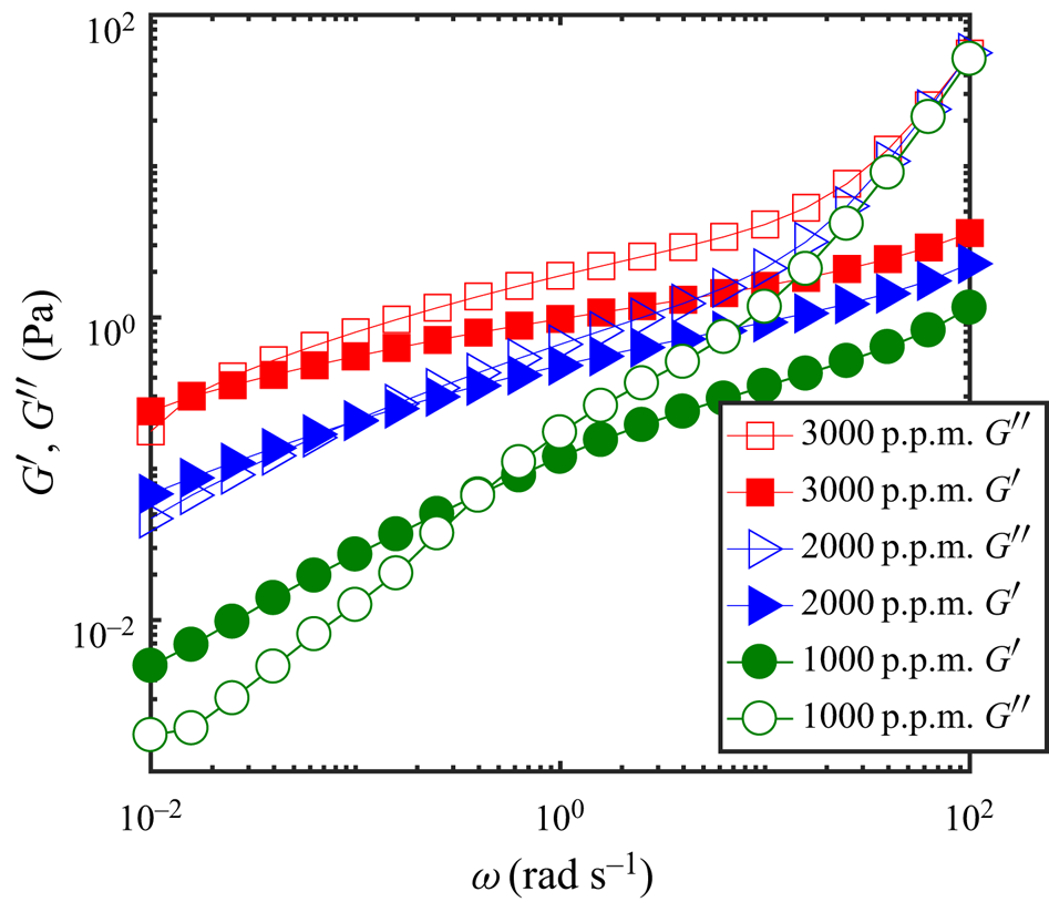
The variation of the storage  $G'$ and loss
 $G''$ modulus versus the shear-rate oscillation
 $\omega$ applied by the rheometer are reported in figure 2 at a strain amplitude
 $\gamma = 1\,\%$ which is, within the linear viscoelastic region, identified through strain sweep tests. The relaxation time
 $\tau _R$ is defined as
 $\tau _R = 1/\omega _c$ according to the Maxwell model where
 $\omega _c$ is the crossover frequency for the
 $G^{\prime }$ and
 $G^{\prime \prime }$ curves. When the concentration increases both
 $G^{\prime }$ and
 $G^{\prime \prime }$ increase and the crossover point shifts to lower shear-rate oscillations. For instance, the relaxation time
 $\tau _R$ is
 $2.5$ s,
 $10.9$ s and
 $63.1$ s for
 $1000$,
 $2000$ and
 $3000$ p.p.m. xanthan concentration, respectively.
Variation of the elastic  $G^{\prime }$ and viscous
 $G^{\prime \prime }$ as a function of the shear oscillation
 $\omega$ for different concentration of xanthan gum solutions.

3.5. Experimental protocol
To observe flow structures corresponding to various  ${Re}$ in the Taylor–Couette geometry, the Reynolds number is slowly increased with time starting from a stationary inner cylinder. Experiments typically lasted approximately
 $6$–
 $10$ h. Temperature measurements of the working fluid before and after an experiment indicated that the temperature change was less than
 $1\,^{\circ } \text {C}$. Details about the experimental procedure are available in supplementary § S3.
4. Primary bifurcation: onset of TVF
Numerical computations were first carried out to investigate endwalls effects. It is found that even for  $L = 10$, there is practically no effect of the endwalls at the middle of the height of the annular space. Details are given in supplementary § S4.
4.1. PIV measurements
In order to check if the viscoelasticity of the fluid plays any role on the onset of Taylor vortices, PIV measurements were performed at  ${Re}$ around
 ${Re}_c$. The increase of the velocity of the inner cylinder follows the protocol given in § 3.5. At
 ${Re}$ below
 ${Re}_c$, PIV measurements did not detect radial or axial velocity. At
 ${Re}$ slightly above
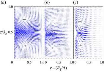
 ${Re}_c$, Taylor vortices are detected. They are illustrated in figure 3, where the velocity field measured just above
 ${Re}_c$, at
 $\epsilon \approx 0.01$, is shown for glycerol solution and xanthan gum solutions at
 $1000$ p.p.m. (
 $n_c = 0.51, \, \lambda = 5.3$) and
 $2000$ p.p.m. (
 $n_c = 0.33, \lambda = 262$). The axial position is scaled with the corresponding wavelength calculated from the distance between two successive outflow boundaries and a single wavelength is represented. It is interesting to note that with increasing shear-thinning effects, Taylor vortices are squeezed against the inner wall (Alibenyahia et al. Reference Alibenyahia, Lemaitre, Nouar and Ait-Messaoudene2012; Agbessi et al. Reference Agbessi, Alibenyahia, Nouar and Choplin2015; Topayev et al. Reference Topayev, Nouar, Bernardin, Neveu and Bahrani2019). The periodicity of the cells around the middle of the annular domain can be estimated from the measurement of the wavelength. This yields wavenumbers
 $k = 3.15 \pm 0.1$ for glycerol solution,
 $k = 3.5 \pm 0.15$ for xanthan gum solution
 $1000$ p.p.m. and
 $k = 4.9 \pm 0.3$ for xanthan gum
 $2000$ p.p.m. These values are in agreement with the linear theory (Topayev et al. Reference Topayev, Nouar, Bernardin, Neveu and Bahrani2019):
 $k_c = 3.1836$,
 $3.4601$ and
 $4.7109$, respectively.
Radial–axial velocity vectors in a radial–axial plane for TVF measured at  $\epsilon \approx 0.01$: (a) glycerol solution with
 $\lambda _z = 2$; (b) xanthan gum solution
 $1000$ p.p.m. with
 $\lambda _z = 1.8$; (c) xanthan gum solution
 $2000$ p.p.m. with
 $\lambda _z = 1.3$. For the same length of a vector, the dimensionless velocity in the panels (b,c) is two times and four times lower than that in the panel (a), respectively.

As already mentioned, above the TVF onset, the maximum of the outflow velocity is larger than the maximum inflow velocity. This is particularly true for shear-thinning fluids (Topayev et al. Reference Topayev, Nouar, Bernardin, Neveu and Bahrani2019). For instance for the xanthan gum  $2000$ p.p.m., the measured ratio between the maximum outflow velocity and the minimum inflow is
 ${\approx }4.3$ at
 $\epsilon = 6.5\,\%$.
The agreement of the measurements with theoretical results (not accounting for elasticity) tend to show that the viscoelastic properties of the fluid do not play any role in the transition to TVF.
4.2. Visualization
Visualization is the most widely used technique to determine the onset of the TVF regime. However, as it will be shown later, some artefacts require special caution particularly for shear-thinning fluids. They are due to the anisotropic shape of the particles used for visualization. Guided by the results of the linear theory, the conclusions of the numerical simulation and the PIV measurements, and after several preliminary experimental tests, we have found that the following three criteria allow us to determine reliably the onset of the TVF: (i) Taylor vortices are first observed in the middle of the apparatus ( $z = L/2$); (ii) the topology remains stable during a sufficiently long time; (iii) there is no variation in the topology after an increase of the velocity of rotation of the inner cylinder by
 $\Delta \varOmega _1 = 0.21\ \text {rad}\ \text {s}^{-1}$.
Glycerol aqueous solution. Experiments were first carried out with a Newtonian fluid. The annular space was filled with  $80\, \%$ glycerol aqueous solution. The velocity of rotation of the inner cylinder was increased slowly from rest as described in the protocol given in § 3.5. Close to the onset of the TVF regime,
 $\Delta \varOmega _1$ was reduced to
 $0.105\ \text {rad}\ \text {s}^{-1}$ (
 $\Delta {Re} = 0.86$) in order to determine accurately the critical Reynolds number. To avoid effects associated with the cylinder ends such as the strong Eckman vortex at the rigid bottom boundary, we focused mainly on the flow structure in the central zone of length
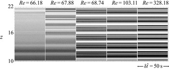
 $12 \, d$. Figure 4 displays the spatiotemporal diagram at five values of
 ${Re}$, each developed over a time span of
 $50 \ \text {s}$. At each time, the image is averaged over 10 pixels in the azimuthal direction. Taking into account the three criteria given above, we find that the transition to TVF occurs at a critical Reynolds number
 $67.88 < {Re}_c^{exp} < 68.74$. This value is in good agreement with that obtained from linear theory assuming infinite cylinders,
 ${Re}_c = 68.2961$. As expected, for the configuration used here,
 $L =32$, the value of the critical Reynolds number for the onset of Taylor vortices is practically unaffected by end effects. This result is in agreement with that of Cole (Reference Cole1976) in the case of a narrow gap (
 $0.85 \leq \eta \leq 0.95$). Based on torque measurements and visual observations, Cole (Reference Cole1976) found that there is no variation of the critical speed for the onset of Taylor vortices, with the annulus length, so that theoretical predictions are applicable for an aspect ratio as small as
 $8$ and probably still smaller. The vortices observed at
 ${Re} = 67.88$ and at
 ${Re} = 66.18$ are to be put on account of end effects, i.e. Eckman vortices penetrate progressively the annular space with increasing
 ${Re}$.
Spatiotemporal diagrams for a  $80\,\%$ by volume of glycerol aqueous solution at
 ${Re} = 66.18$, 67.88, 68.74, 103.11 and
 ${Re} = 328.18$. They are constructed from images taken at 10 frames
 $\textrm {s}^{-1}$. Note that for a Newtonian fluid with
 $\eta = 0.4$,
 ${Re}_c = 68.2965$. At
 ${Re} = 66.18$,
 $50\ \text {s} = 573.05 \, d / (R_1 \varOmega _1)$.

In order to determine the critical wavenumber  $k_c^{exp}$, a Fourier transform has been applied to the greyscale spatiotemporal diagram
 $I( z) = \sum _{k} \bar {I}(k) \exp (\textrm {i} k z)$ corresponding to
 ${Re} = 68.74$. The maximum of the squared modulus of the Fourier coefficient
 $|\bar {I}|^2$ is reached at
 $k = k_c^{exp}= 3.27$ which is close to the critical axial wavenumber
 $k_c = 3.1834$ obtained from the linear stability analysis. Actually, one has to note that for a finite system, only discrete states with an integer number of vortices can occur. With one rigid and one free boundary, our system normally contains an odd number of vortices (
 $2 N + 1$) (Linek & Ahlers Reference Linek and Ahlers1998; Watanabe & Toya Reference Watanabe and Toya2012). We designate by
 $k_c^{finite}$ the closest value to
 $k_c$ compatible with an odd number of vortices. We obtain
 $k_c^{finite} = 3.24$, which is very close to our experimental result
 $k_c^{exp}=3.27$. The stationarity of TVF is evident from figure 4.
Once the primary bifurcation is reached, the velocity of rotation of the inner cylinder was increased gradually by small steps following the protocol given in § 3.5. Space–time diagrams obtained from visualization at  ${Re}$ between
 $68.74 \, ({Re}_c^{exp})$ and
 $328.18 \, (4.8 \, {Re}_c^{exp})$ do not present any visible variation, as is shown in figure 4. The wavenumber remains constant with
 $k = k_c^{exp} = 3.27$. This is in agreement with experimental observations of Snyder & Lambert (Reference Snyder and Lambert1966) and Burkhalter & Koschmieder (Reference Burkhalter and Koschmieder1973) using an apparatus of radius ratio
 $\eta = 0.5$ and an aspect ratio
 $L \approx 30$ and increasing quasisteadily the Reynolds number. According to Guo & Finlay (Reference Guo and Finlay1991), this suggests that perturbations with
 $k = k_c$ grow faster than others and become dominant in the fully vortex flow. However, the flow structure is modified. Indeed, PIV measurements show that at
 ${Re}$ sufficiently far from
 ${Re}_c$, the centre of vortices moves towards the outflow boundaries and the outer cylinder wall, in agreement with the numerical observations of Fasel & Booz (Reference Fasel and Booz1984).
Aqueous solution of xanthan gum. The onset of the TVF regime in aqueous solutions of xanthan gum used is illustrated in the case corresponding to a concentration of  $2000$ p.p.m. The transition to TVF regime for
 $1000$ and
 $3000$ p.p.m. is described by the supplementary figures F3 and F4.
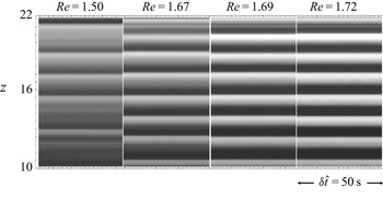
Figure 5 shows spatiotemporal diagrams for aqueous solution of xanthan gum at  $2000 \ \text {p.p.m.}$, with
 $n_c = 0.34$ and
 $\lambda = 197$. Stationary patterns are first observed at
 ${Re} = 1.12$, much lower than the critical Reynolds number predicted by the linear theory,
 ${Re}_c = 1.6944$. These patterns are illustrated by the space–time plot shown in the left-hand subpanel of figure 5. They account for a variation of the orientation of reflective particles along the axial position which can be related to Taylor-like vortices. At
 $Re = 1.69$, the three criteria for the onset of TVF are satisfied. The experimental Reynolds number for the onset of TVF,
 $1.67 < {Re}_c^{exp} < 1.69$ is in agreement with the linear theory. Applying a fast Fourier transform (FFT) to the space–time plot corresponding to
 ${Re} = 1.69$, it is found that the most energetic mode is obtained at
 $k = k_c^{exp} = 4.37$. This value is again in very good agreement with that obtained using a linear stability analysis,
 $k_c = 4.5160$. If we take into account the finite length of the system, a closer value is obtained,
 $k_c^{finite} = 4.4156$.
Space–time diagrams of xanthan gum  $2000 \ \text {p.p.m.}$ for
 ${Re} = 1.5, 1.67, 1.69$ and
 $1.72$. The rheological parameters are
 $n_c = 0.34$,
 $\lambda = 197$. For this case, the linear theory gives
 ${Re}_c = 1.6944$. At
 ${Re} = 1.5$,
 $50\ \text {s} = 1099 \, d / (R_1 \varOmega _1 )$.

The values of  $Re_c$,
 $Re_{c,exp}$,
 $k_c$,
 $k_{c,exp}$ and
 $k_{c,finite}$ for aqueous solution of glycerol and aqueous solutions of xanthan gum used are provided in supplementary table T6.
4.3. Discussion
From the experimental results, the following points can be underlined. (i) For the geometrical configuration used, the critical conditions are practically not affected by the end effects in agreement with Cole (Reference Cole1976). (ii) The critical Reynolds and axial wavenumbers obtained experimentally are in good agreement with the linear theory assuming a purely viscous shear-thinning fluid. (iii) No sign of elastic instability such as ribbon, spiral vortices or diwhirls (Groisman & Steinberg Reference Groisman and Steinberg1998; Crumeyrolle, Mutabazi & Grisel Reference Crumeyrolle, Mutabazi and Grisel2002) was observed despite the large values of the Deborah number  $De$ and the elasticity number
 $El$ found. For instance, for the xanthan gum at
 $2000$ p.p.m. we have
 $De = 120.2$ and
 $El = 71.1$. The Deborah number is defined as the product of the relaxation time with a nominal shear rate (Cagney & Balabani Reference Cagney and Balabani2019b; Cagney et al. Reference Cagney, Lacassagne and Balabani2020)
 $\varOmega _1 R_1/d$ and the elasticity number as
 $El=De/Re$. Note that Groisman & Steinberg (Reference Groisman and Steinberg1998) did not observe any sign of elastic instability for aqueous solutions of xanthan gum up to
 $De = 600$, the maximum value reachable in their experiments. (iv) For sufficiently strong shear-thinning effects, patterns which can be related to counter-rotating vortices are observed at
 ${Re}$ much lower than
 ${Re}_c^{exp}$. The value of
 ${Re}$ at which these patterns appear decreases with increasing shear-thinning effects. Elçiçek & Güzel (Reference Elçiçek and Güzel2020) have also reported, from visualization experiments, the existence of axisymmetric vortices at
 $\epsilon \approx -15\,\%$ (before TVF regime, figure 10 in their paper) and they attributed their existence to Eckman vortices.
Based on the point (i) and the supplementary figure F2, we think that the patterns observed at  ${Re}$ much below
 ${Re}_c$ are not induced by the vortices generated by the endwall boundary condition. These patterns might be ascribed to the anisotropic shape of the particles, since PIV measurements using spherical particles did not detect radial or axial velocity at
 ${Re}$ much below
 ${Re}_c$. The only difference between the visualization experiments and the PIV measurements is the shape of the particles. In order to clarify the mechanisms behind the appearance of the banded structures, additional investigations are planned. One possibility is to analyse the motion of anisotropic particles in a Couette flow of a shear-thinning fluid with realistic boundary conditions. Another possibility is to extend the theoretical study of Gillissen & Wilson (Reference Gillissen and Wilson2018) to the case of a shear-thinning fluid. These authors demonstrated theoretically that suspensions of disks in a Newtonian fluid have a destabilizing effect in a CCF. This destabilization is due to anisotropic viscous stress induced by suspended disk shaped particles. Furthermore, it is shown (Gillissen & Wilson Reference Gillissen and Wilson2018; Gillissen et al. Reference Gillissen, Cagney, Lacassagne, Papadopoulou, Balabani and Wilson2020) that the critical Reynolds number for the onset of instability of the CCF decreases strongly with increasing the concentration of particles.
5. Secondary bifurcations
5.1. Newtonian fluid: instability to travelling azimuthal wave mode
Visualization experiments show that in the TVF regime, Taylor vortices are stationary and their axial periodicity is the same as at the onset (figure 4). At  ${Re} = {Re}_s^{exp} = 361 = 5.28 \, {Re}_c$, a secondary instability occurs with a transition from steady axisymmetric Taylor vortices to time-dependent non-axisymmetric flow. Typical spatiotemporal diagrams of reflected light intensity obtained, in this regime, at
 ${Re} = 361 \, (5.28 \, {Re}_c)$ and
 ${Re} = 452 \, (6.58 \, {Re}_c )$ are shown in supplementary figures F5 and F6. Applying the two-dimensional FFT to spatiotemporal diagrams, it is possible to obtain the axial wavenumber and the frequency of oscillations. The axial wavenumber remains the same as in TVF regime,
 $k \approx k ^{finite}_c = 3.27$. The period
 $T$ of oscillations in non-dimensional time units and the ratio of the frequency of oscillations to the inner cylinder frequency at different
 ${Re}$ is given in table 1. It can be noted that in the regime called here wavy vortex flow I (WVF I), the period (frequency) of oscillations increases (decreases) as the Reynolds number is increased. This time-dependent flow regime is observed for
 ${Re}$ ranging from
 $361 \, (5.28 \, {Re}_c)$ to
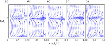
 $472 \, ({\approx }6.9\, {Re}_c)$. Additional information about this regime is obtained from PIV measurements. Figure 6 shows the instantaneous velocity field in the radial–axial plane at
 ${Re} = 444 \, (6.5 \, {Re}_c)$ through one cycle. One period is represented. The axial motion of the vortices is evident based on the location of the vortex centres marked by a cross. One can also observe that: (i) the outflow boundary oscillates with a very small amplitude; (ii) the inflow boundary has a significant amplitude of oscillations; (iii) the radial outflow is much stronger than the radial inflow. By numbering the vortices 1 to 3 from the bottom, and analysing the orientation of vectors velocity in different panels of figure 6, it can be shown that there is a weak transfer of the fluid from the vortex 2 to the vortex 1 in figure 6(b) and from the vortex 1 to the vortex 2, in figure 6(d). Of course, the net volume of fluid transferred axially over one cycle must be zero.
Period  $T$ of oscillations in non-dimensional time units and ratio of the frequency of oscillations to the inner cylinder frequency
 $f_i$.

Aqueous glycerol solution. Instantaneous radial–axial velocity vectors in radial–axial plane for WVF I at  ${Re}= 444 \, (6.5 \, {Re}_c)$. The time progresses from left to right through one cycle of an azimuthal wave passing the measurement plane: (a)
 $t = 0$; (b)
 $t = 5.3 (d/R_1 \varOmega _1 )$; (c)
 $t = 13.25 (d/R_1 \varOmega _1 )$; (d)
 $t = 21.2 (d/R_1 \varOmega _1 )$; (e)
 $t = 26.5 (d/R_1 \varOmega _1 )$.

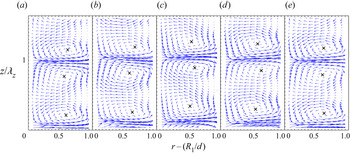
At  ${Re} = 472 \approx 6.9 \, {Re}_c$, an abrupt increase (decrease) in period (frequency) of oscillations occurs as indicated in table 1 associated with an abrupt increase in the amplitude oscillations as shown in supplementary figure F7. The axial wavenumber is not modified
 $k = k_c^{finite} \approx 3.27$. The flow field through one cycle of an azimuthal wave passing the measurement plane represented in figure 7 is quite similar to that described previously and will be called here wavy vortex flow II (WVF II). However, the oscillations’ amplitude of the outflow boundary is stronger than it was previously, as well as the transfer of the fluid between vortices 1 and 2 in figures 7(a), 7(c) and 7(e). The WVF II has the same features as the WVF described by Wereley & Lueptow (Reference Wereley and Lueptow1998) for a narrow gap geometry (
 $\eta = 0.83$). However, in their case, the experimental results do not show any jump in the frequency nor in the amplitude of the oscillations.
Aqueous glycerol solution. Instantaneous radial–axial velocity vectors in radial–axial plane for WVF II at  ${Re} = 478 \, (7 \, {Re}_c)$. The time progresses from left to right through one cycle of an azimuthal wave passing the measurement plane: (a)
 $t = 0$; (b)
 $t = 14.4 (d/R_1 \varOmega _1 )$; (c)
 $t = 28.8 (d/R_1 \varOmega _1 )$; (d)
 $t = 43.2 (d/R_1 \varOmega _1 )$; (e)
 $t = 51.8 (d/R_1 \varOmega _1 )$.

The stage WVF I observed here experimentally was not detected by Razzak et al. (Reference Razzak, Khoo and Lua2019) using a numerical simulation with periodic boundary conditions and  $\eta = 0.5$. One might be also tempted to make a connection between outward WVF I and the inward flow oscillations observed by Lorenzen et al. (Reference Lorenzen, Pfister and Mullin1983) for
 $11.5 \leq L \leq 15$. However, in their case the outflow boundary is flat and the frequency of oscillations is constant with increasing
 $Re$ unlike our WVF I. This discrepancy with the literature shows again that the radius ratio and the aspect ratio are crucial parameters in the wavy instability.
5.2. Shear-thinning fluids: creation and merging of vortices
For the shear-thinning fluids, visualization and PIV measurements, as well as axisymmetric numerical simulations used, show that starting from a secondary critical Reynolds number,  ${Re}_s$, the regular arrangement of Taylor vortices with an axial wavenumber
 $k = k_c$ becomes unstable in a fundamentally different way from that discussed in the Newtonian case, since the flow remains axisymmetric. The instability is characterized by a creation of a new pair of vortices in the inflow region, where the inward flow is weak, causing a local increase of the wavenumber. This new state is in its turn unstable and two vortex pairs merge to form one pair reducing the wavenumber. This process of creation and annihilation of vortex pairs repeats continuously. The axial position at which a new vortex pair is created is random. Furthermore, once a new extra vortex pair appears, or once two vortex pairs start to merge to form one pair, neighbouring vortex pairs will move modifying the wavenumber and consequently the axial positions of the following events of creation and merging. A complex pattern may then result. Note also that it is possible to have more than one defect in the system.
5.2.1. Results of axisymmetric numerical simulations
As mentioned in the supplementary § S1, a continuation method is used to solve the unsteady axisymmetric momentum equations. Each new simulation is started with the converged solution of the steady regime corresponding to the closest set of parameters as initial condition. This procedure is followed before and after the onset of TVF. In the TVF regime, Taylor vortices are steady and their axial periodicity remains the same as at the onset. As we have seen, with increasing Reynolds number, the outflow becomes stronger than the inflow and the extent of the inflow zone where the vorticity is low increases accordingly.
For a Carreau fluid with  $n_c = 0.5, \, \lambda = 200$ and periodic boundary conditions in the axial direction, the steady axisymmetric vortices lose their stability at
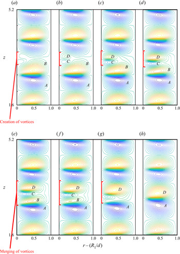
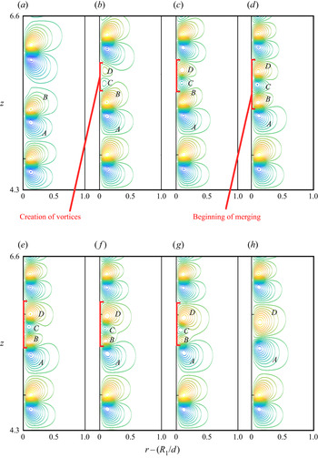
 ${Re} = 1.69 \, {Re}_c$. A continuous creation and merging of vortices is observed. This is illustrated by figure 8 where contours of stream functions for three base vortex pairs are represented at different times. The choice of three base vortex pairs rather than the whole system is adopted only for a better illustration of the creation and merging process. At
 $t = T_0$ (figure 8a), a new vortex pair, denoted
 $C$ and
 $D$, emerges. It grows radially and reaches its maximum strength at
 $t \approx T_0 + 25$ (figure 8d). The development of the vortices leads to a local increase of the wavenumber. At
 $t = T_0 + 36$ (figure 8e) the merging process starts: two vortices
 $B$ and
 $C$ in figure 8(e,f) appear to collide and disappear completely at
 $t = T_0 + 64$. A new pair formed by the vortices
 $A$ and
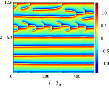
 $D$ is obtained. A short time after, a new vortex pair emerges between two other base vortex pairs, it increases radially then merges with one of the adjacent base vortex pairs by the same mechanism. Another illustration of creation and merging events is given in figure 9. The distribution of the azimuthal vorticity along the line
 $r = R_1/d + 0.44$ (passing near the centre of vortices) is represented as a function of time. It can be observed how the vortices
 $B$ and
 $C$ are weakened and then annihilated. A representation of the vorticity distribution on a longer interval of time and for the whole system in figure 10 shows the repetitive appearance of creation and merging of vortex pairs. Simultaneous defects may occur at the same time. A similar phenomenon is observed for fixed bottom endwall and stress-free conditions at the top endwall, the secondary critical Reynolds number
 ${Re}_s = 1.67 \, {Re}_c$ is also practically the same to that obtained for periodic boundary conditions.
Secondary instability for a Carreau fluid with  $n_c = 0.5$,
 $\lambda = 200$ at
 ${Re} = 1.67 \, {Re}_c$. Periodic boundary conditions in the axial direction, with
 $\lambda _z = 1.7974, \, L = 7 \, \lambda _z = 12.582$. Contours of stream function at different times: (a)
 $t = T_0$; (b)
 $t = T_0 + 6$; (c)
 $t = T_0 + 15$; (d)
 $t = T_0 + 30$; (e)
 $t = T_0 + 36$; (f)
 $t = T_0 + 45$; (g)
 $t = T_0 + 57$; (h)
 $t = T_0 + 64$.

Secondary instability for a Carreau fluid with  $n_c = 0.5$,
 $\lambda = 200$ at
 ${Re} = 1.69 \, {Re}_c$. Periodic boundary conditions in the axial direction with
 $\lambda _z = 1.7974, \, L = 7 \, \lambda _z = 12.582$. Distribution of the azimuthal vorticity along the line
 $r =R_1/d + 0.44$ as a function of time: close-up on three pairs of vortices.

Secondary instability for a Carreau fluid with  $n_c = 0.5$,
 $\lambda = 200$ at
 ${Re} = 1.69 \, {Re}_c$. Periodic boundary conditions in the axial direction with
 $\lambda _z = 1.7974, \, L = 7 \, \lambda _z = 12.582$. Distribution of the azimuthal vorticity along the line
 $r =R_1/d + 0.44$ as a function of time.

With increasing shear-thinning effects, the range of Reynolds numbers for which the Taylor vortices remain stable shrinks. For instance, for  $n_c = 0.2, \, \lambda = 200$, Taylor vortices lose their stability at Reynolds number
 $1.07 \, {Re}_c < {Re}_s < 1.08 \, {Re}_c$. Similar events of creation and merging of vortices are observed as shown in figure 11 where contours of stream functions are shown at different times at
 ${Re} = 1.08 \, {Re}_c$. A new pair of vortices
 $C$ and
 $D$ forms at
 $t \approx T_0 + 20$. This grows in size, and reaches a maximum at
 $t \approx T_0 + 70$. From this time, two vortices of opposite sign of vorticity
 $C$ and
 $B$ appear to collide and then cancel at
 $t \approx T_0 + 117$. A new pair of vortices
 $A$ and
 $D$ is obtained. Note that the process lasts longer than for
 $n_c = 0.5, \, \lambda = 200$. The repetitive appearance of creation and merging of vortex pairs is illustrated in figure 12 by the evolution of the azimuthal vorticity along the line
 $r = R_1/d + 0.123$ in time. It is interesting to observe how the process of creation and merging modifies the local wavenumber of the neighbouring vortices and consequently the following events of creation and merging. For
 $n_c = 0.2$ and
 $\lambda = 200$, and for both types of boundary conditions, we observed up to a maximum of four defects at the same time. We think that the number of simultaneous defects depends on the aspect ratio.
Secondary instability for a Carreau fluid with  $n_c = 0.2$,
 $\lambda = 200$, fixed bottom endwall, stress-free at the top endwall at
 ${Re}=1.08\, {Re}_c$. Contours of stream function at different times: (a)
 $t = T_0$; (b)
 $t = T_0 + 20$; (c)
 $t = T_0 + 49$; (d)
 $t = T_0 + 69$; (e)
 $t = T_0 + 96$, (f)
 $t =$; (g)
 $t = T_0 + 110$; (h)
 $t = T_0 + 117$.

Secondary instability for a Carreau fluid with  $n_c = 0.2$,
 $\lambda = 200$, fixed bottom endwall, stress-free at the top, at
 ${Re} = 1.08 \, {Re}_c$. Distribution of the azimuthal vorticity along the line
 $r =R_1/d + 0.123$ as a function of time.

Because of repetitive creation and merging processes, the torque applied on the inner cylinder experiences fluctuations. In figure 13 we have plotted the variation of the ratio of the torque to that obtained in a purely Couette flow as a function of time. The simulation parameters are  $n_c = 0.5, \lambda = 200, Re = 1.69 \, Re_c$, periodic boundary conditions in the axial direction and
 $L = 8 \, \lambda _z$. The dashed line before
 $t = 0$ is the converged solution at
 ${Re} = 1.62 \, {Re}_c$. Figure 14(a) is a close-up of the curve
 $C(t)/C_b$ showing when creation and merging events occur. Examining
 $C(t)/C_b$ and the velocity field, we have placed, on the curve
 $C(t)/C_b$, letters
 $C, D$ and
 $M$ for torque at times of creation of a new pair of vortices, of full development of the new pair of vortices and of the end of merging, respectively. It can be observed that
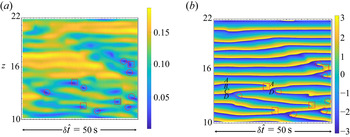
 $C(t)/C_b$ increases when the new pair of vortices rises and decreases when the merging process is underway. It happens, that we have a creation of two pairs of vortices at the same time and at two different axial positions, with different times of raising and merging. Similar results are obtained using fixed bottom endwall and stress-free conditions at the top endwall (figure 14b). Starting from
 $t = 1000$, a Fourier transform of the plot in figure 10 presents a dominant peak at
 $f = 0.0153$ corresponding to a period
 $T = 65$. It is visible in figure 14(a) and can be related to the frequency of generation of defects along the line
 $z \approx 7$ in figure 10. Similar analysis applies to figure 14(b). A dominant peak at
 $f = 0.007$ corresponding to
 $T \approx 140$ is obtained and can be related in the generation of defects in figure 12.
Secondary instability for a Carreau fluid with  $n_c = 0.5$,
 $\lambda = 200$. Variation of the ratio of the torque to that obtained for a purely Couette flow with periodic boundary conditions at
 ${Re} = 1.69 \, {Re}_c$. The dashed line before
 $t = 0$, is the converged solution at a lower Reynolds number.

Secondary instability for a Carreau fluid. Variation of the ratio of the torque to that obtained for a purely Couette flow. Panel (a) is for  $n_c = 0.5$,
 $\lambda = 200$,
 ${Re} = 1.69 \, {Re}_c$, periodic boundary conditions in the axial direction. Panel (b) is for
 $n_c = 0.2$,
 $\lambda = 200$,
 ${Re} = 1.08 \, {Re}_c$, fixed bottom endwall and stress-free at the top endwall.

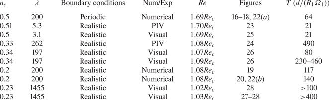
It is not surprising to observe that the period of creation and merging is longer for a Carreau fluid with  $n_c = 0.2, \, \lambda = 200$ than that for
 $n_c = 0.5, \lambda = 200$, since with increasing shear-thinning effects, the inward flow in the inflow region becomes weaker. The same tendency is observed for fixed
 $n_c$ and larger
 $\lambda$. This may explain the difference in time of creation and merging of vortices between figures 8 and 15.
Xanthan gum  $1000$ p.p.m. with
 $n_c = 0.51, \, \lambda = 5.3$. Velocity field in the plane
 $(r, z)$ with (a)
 $\hat {t} = T_0$, (b)
 $\hat {t} = T_0 + 0.2 \ \textrm {s} = T_0 + 2.1 \, d/(R_1 \varOmega _1)$, (c)
 $\hat {t} = T_0 + 1.5 \ \textrm {s} = T_0 + 15.8 \, d/(R_1 \varOmega _1)$, (d)
 $\hat {t} = T_0 + 1.7 \ \textrm {s} = T_0 + 17.9 \, d/(R_1 \varOmega _1)$, (e)
 $\hat {t} = T_0 + 2 \ \textrm {s} = T_0 + 21 \, d/(R_1 \varOmega _1)$.

5.2.2. Experimental results: PIV measurements and visualization
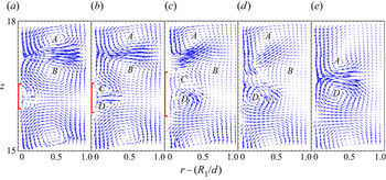
Instability of Taylor vortices in shear-thinning fluids was also investigated experimentally by PIV measurements and by visualization. In agreement with the numerical simulation, a secondary bifurcation sets in at  ${Re} = {Re}_s$ depending on the rheological properties of the fluid. The fluid stays axisymmetric but becomes time dependent with repetitive sequences of creation and merging of vortices. Such a process is shown in figure 15 where we have plotted, for xanthan gum 1000 p.p.m. with
 $n_c = 0.51$ and
 $\lambda = 5.3$, snapshots of an instantaneous velocity field in the vertical plane
 $(r, z)$ at
 ${Re} = 16.5 = 1.7 \, {Re}_c$. Emergence of a new vortex pair at the inner wall is evident in figure 15(a). It grows in size with increasing time as indicated by figure 15(b,c). The new vortex pair and one base vortex pair collide. The vortices
 $B$ and
 $C$ of opposite sign of vorticity in figure 15(d) weaken and disappear. In figure 15(e) a new vortex pair is formed by the vortices
 $A$ and
 $D$. The process of creation and merging lasts approximately
 $2\ \text {s} = 21\, d/(R_1 \varOmega _1)$ and repeats continuously. During this process, several defects exist out of the measurement zone. Comparison between figure 15(a) and figure 15(e) shows an axial shift of the outflow boundaries which will lead to a modification of the local axial wavenumber of the neighbouring vortices.
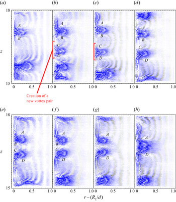
Qualitatively, the same phenomena are observed for higher concentration of xanthan gum, i.e. for stronger shear-thinning effects. However, three fundamental differences have to be stressed, by comparison with xanthan gum  $1000$ p.p.m.: (i) the outward radial flow is much stronger and narrower than the radial inward flow; (ii) the new vortex pair reaches practically the same size as the base vortex pair; and (iii) the time before merging is much larger. An illustration is given in figure 16 where the flow field in the
 $(r,z)$ plane, obtained for xanthan gum 2000 p.p.m. with
 $n_c = 0.33, \, \lambda = 262$ at
 ${Re} = 1.08 \, {Re}_c$, is represented at different times. A new vortex pair
 $C$,
 $D$ is formed in figure 16(b). It is bigger in figure 16(c). Its development is accompanied by a splitting of the two neighbouring vortex pairs. It remains aligned with the base vortex pairs for a significant amount of time, here
 $30\ \textrm {s} \approx 350 \, d / (R_1, \varOmega _1 )$, before merging. The process of merging by collision starts from figure 16(d). The vortices
 $B$ and
 $C$ weaken and disappear in figure 16(e–g). A new vortex pair
 $A$,
 $D$ is formed in frame (h). The creation and merging process lasts
 $42 \ \textrm {s} = 490 \, d / (R_1 \varOmega _1)$, much longer than xanthan gum
 $1000$ p.p.m., in addition more defects may appear at the same time.
Xanthan gum  $2000$ p.p.m. with
 $n_c = 0.33, \, \lambda = 262$. Velocity field in the plane
 $(r, z)$ with (a)
 $\hat {t} = T_0$, (b)
 $\hat {t} = T_0 + 1.5 \ \textrm {s} = T_0 + 17.5 \, d/(R_1 \varOmega _1)$, (c)
 $\hat {t} = T_0 + 3.3 \ \textrm {s} = T_0 + 38.7 \, d/(R_1 \varOmega _1)$, (d)
 $\hat {t} = T_0 + 33.1 \ \textrm {s} = T_0 + 385 \, d/(R_1 \varOmega _1)$, (e)
 $\hat {t} = T_0 + 38.1 \ \textrm {s} = T_0 + 443 \, d/(R_1 \varOmega _1)$, (f)
 $\hat {t} = T_0 + 39.2 \ \textrm {s} = T_0 + 456 \, d/(R_1 \varOmega _1)$, (g)
 $\hat {t} = T_0 + 40.4 \ \textrm {s} = T_0 + 470 \, d/(R_1 \varOmega _1)$, (h)
 $\hat {t} = T_0 + 42.1 \ \textrm {s} = T_0 + 490 \, d/(R_1 \varOmega _1)$.

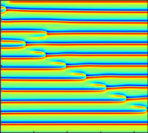
In the visualization experiments, the flow is recorded in the front view plane with a CCD camera ( $10\ \textrm {frames}\ \textrm {s}^{-1}$). These experiments allow us: (i) to determine the secondary critical Reynolds number from which the stationary TVF regime bifurcates towards an unsteady regime where creation and merging of vortices happens repetitively; (ii) to provide another view of the creation and merging process; and (iii) to account for the complexity of the patterns with increasing Reynolds number because of the nonlinear interactions between vortex pairs.
For xanthan gum 1000 p.p.m. with  $n_c = 0.5, \, \lambda = 3.1$, the secondary critical Reynolds number found experimentally is
 $1.65 \, {Re}_c < {Re}_s < 1.7 \, {Re}_c$, with
 $Re_c = 10.9823$. It is quite close to that obtained numerically for a higher value of
 $\lambda$ and lower aspect ratio. Visualization of creation and merging events is tricky as expected from the analysis of figure 15, in addition the process is fast (
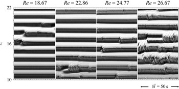
 ${\approx }3 \ \textrm {s}$). Figure 17 shows spatiotemporal diagrams of the reflected light intensity at different values of
 ${Re}$. In the subpanel where
 ${Re} = 18.67$, emergence of a small bright spot in a dark zone at
 $z \approx 16$ and
 $z \approx 18$ corresponds to a creation of a new vortex pair. Merging of the new bright spot with a large bright band corresponds to merging of vortices. It is followed by an abrupt axial shift of the outflow boundary. In the subpanel where
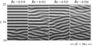
 ${Re} = 22.86$, continuous creation and merging events occur at
 $z \approx 12$, probably similar to the numerical simulations in figure 10. As the Reynolds number increases, the defects become more frequent and complex patterns arise. Nevertheless, the bright bands remain horizontal.
Xanthan gum  $1000$ p.p.m.,
 $n_c = 0.5$ and
 $\lambda = 3.1$. Spatiotemporal diagrams at different Reynolds numbers: front view of repetitive creation and merging events. At
 ${Re} = 18.67$,
 $50 \ \textrm {s} = 342 d / (R_1 \varOmega _1)$.

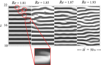
For xanthan gum  $2000$ p.p.m. with
 $n_c = 0.34$ and
 $\lambda = 197$, the onset of the secondary instability occurs earlier than for xanthan gum
 $1000$ p.p.m. Experimentally, we have
 $1.05 \, {Re}_c < Re_s < 1.07 \, {Re}_c$, with
 ${Re}_c = 1.6916$. Front view of repetitive sequences of creation and merging of vortices is illustrated in figure 18, where spatiotemporal diagrams are shown at different values of
 ${Re}$. As previously, at
 ${Re}= {Re}_s \approx 1.81$, one observes emergence of a weakly bright spot in a dark region, corresponding to emergence of new vortex pairs, at different axial positions, (here,
 $z \approx 18$,
 $19$ and
 $20$ highlighted by circles). They grow in size and merge with a larger neighbouring base vortex pair after a quite short time. The creation and merging last approximately
 $7 \ \textrm {s} = 80 \, d/(R_1 \varOmega _1 )$. At the end of the process, the axial position of the vortices is abruptly shifted axially. This axial shift of the vortices modifies the local wavenumber and favours subsequently the formation of a new vortex pair, similarly as in figure 12. By increasing slightly the Reynolds number, it is observed that: (i) the formation of the new vortex pair and its development leads to a significant splitting of the neighbouring vortices, as shown in the frame
 ${Re} = 1.93$ at
 $z \approx 12$; (ii) the new vortex pair may remain aligned for some time, (
 $20 - 40\ \textrm {s} = 230 - 460 \, d/(R_1 \varOmega _1))$ before merging; and (iii) the bright bands are no longer horizontal, i.e. their axial position evolves, as a consequence of a number of defects splitting and merging simultaneously.
Xanthan gum  $2000$ p.p.m.,
 $n_c = 0.34$ and
 $\lambda = 197$. Spatiotemporal diagrams at different Reynolds numbers: front view of repetitive creation and merging events. At
 ${Re} = 1.81$,
 $50 \ \textrm {s} = 523 \, d / (R_1 \varOmega _1)$. The insert is a close-up on the emergence of a weakly bright spot in a dark region.

At still higher concentration of xanthan gum, the onset of creation and merging of vortices occurs very close to  $Re_c$, i.e. the range of stable TVF shrinks strongly. For xanthan gum
 $3000$ p.p.m. with
 $n_c = 0.23, \, \lambda = 1255$, creation and merging of vortices happen at
 ${Re} = 1.02 \, {Re}_c$. For a slightly larger Reynolds number, the phenomena described previously, i.e. (i) the increasing number of defects and (ii) the non-horizontal bright bands, become more pronounced as shown in figure 19. However, the creation and merging of vortices is the main mechanism that drives the flow structure. It can be still better illustrated by applying a complex demodulation technique to the reflected light intensity
 $I(z, t)$ (Bot & Mutabazi Reference Bot and Mutabazi2000; Crumeyrolle et al. Reference Crumeyrolle, Latrache, Mutabazi and Ezersky2005). The real signal
 $I(z, t)$ is transformed in its complex equivalent expression by means of a Hilbert transform (Bot & Mutabazi Reference Bot and Mutabazi2000; Crumeyrolle et al. Reference Crumeyrolle, Latrache, Mutabazi and Ezersky2005). In practice, the complex demodulation is performed by computing a two-dimensional FFT of
 $I(z, t)$, keeping the most energetic modes and performing an inverse FFT. The modulus
 $|A(z,t)|$ and the phase
 $\phi (z,t)$ of the complex signal are then determined. Figure 20 shows such a result for xanthan gum 3000 p.p.m. at
 ${Re} = 0.52$. The phase varies from
 $- {\rm \pi}$ (dark colour) to
 $+ {\rm \pi}$ (bright colour). The phase jump from
 $- {\rm \pi}$ to
 $+ {\rm \pi}$ at the boundary between dark and bright colours corresponds to the boundary between two counter-rotating vortices. The main feature of the space–time diagrams displayed in figure 20 is the occurrence of topological defects: points where the amplitude
 $|A|$ vanishes (dark points in the amplitude space time diagram) and the phase is no longer defined. Two types of defects are clearly observed. The first one shown by a square is a merging by two vortex pairs. The phase jumps by
 $- 2 {\rm \pi}$ after a loss of one pair of rolls. The second type of defect is shown by a circle, where the phase jumps by
 $+ 2 {\rm \pi}$ corresponds to a creation of one vortex pair. The process described previously can again be observed in figure 20(b): two vortices
 $B$ and
 $C$ weaken with time, then disappear and a new vortex pair
 $A$ and
 $D$ is formed.
Xanthan gum  $3000$ p.p.m.,
 $n_c = 0.23$ and
 $\lambda = 1255$. Spatiotemporal diagrams at different Reynolds numbers. At
 ${Re} = 0.519$,
 $50 \ \textrm {s} = 809\, d / (R_1 \varOmega _1)$.

Xanthan gum  $3000$ p.p.m.,
 $n_c=0.23$ and
 $\lambda =1255$. Complex demodulation of a spatiotemporal diagram at
 ${Re} = 0.521$: (a) amplitude demodulation dark zones corresponds to the core of the defects where the amplitude vanishes; (b) phase demodulation. Circles and squares show the position of creation and merging processes, respectively.

Our experimental and numerical results are summarized in figure 21 and table 2. In figure 21, we have reported the stability diagram in the plane  $(\epsilon = ({Re} - {Re}_c)/ {Re}_c, n_c )$. The primary bifurcation occurs at
 $\epsilon = 0$ and the TVF regime is stable when
 $0 < \epsilon < \epsilon _s$, i.e.
 ${Re}_c < {Re} < {Re}_s$. The variation of
 $\epsilon _s$ with
 $n_c$ is shown by a dashed line. From
 $\epsilon > \epsilon _s$, the TVF regime is no longer stable. It is interesting to note that there is a quite good agreement between the numerical and the experimental results even if the experimental aspect ratio is three times higher than the numerical one.
Stability diagram of the TVF regime for a Carreau fluid with  $\eta = 0.4$ in the plane
 $(\epsilon = ({Re} - {Re}_c) / {Re}_c), \, n_c )$. The thin dashed line (drawn as a guide for the eye) joins the experimental results represented by filled circles. Numerical results are represented by a filled triangle for realistic boundary conditions and filled diamonds for periodic boundary conditions.

Durations  $T$ (last column) between creation and merging process for different rheological parameters: numerical and experimental results.

In table 2, we have reported the times  $T$ between creation and merging. Close to the onset of secondary bifurcation, globally,
 $T$ increases with increasing shear-thinning effects. As the Reynolds number increases further from
 $Re_s$, this process lasts significantly longer time, particularly for low
 $n_c$.
Remark. For a Carreau fluid with  $n_c = 0.5$ and
 $\lambda = 3.1$, a reduction of the wavelength was observed at two Reynolds numbers
 $Re = 14.48$ and
 $16.77$ below
 ${Re}_s$. In these cases, a new steady state with an additional vortex pair appears. Such reduction of the wavelength has also been detected by PIV measurement using spherical particles. Therefore, one may conjecture that this reduction of the wavelength is not an artefact induced by the anisotropic shape of the particles used in flow visualization.
Creation, propagation and annihilation of vortices was observed by Hoffmann et al. (Reference Hoffmann, Altmeyer, Heise, Abshagen and Pfister2013) in a Newtonian fluid, in the case of a short Taylor–Couette system ( $L = 4$ and
 $L = 8$) with counter-rotating cylinders, non-rotating end walls and before the centrifugal instability. The radius ratio is
 $\eta = 0.5$. In their study: (i) the vortices are generated by the shear flow near the Ekman cells; and (ii) the phenomenon of creation and merging is not observed in the case of periodic boundary conditions. The physical mechanisms involved in their study are fundamentally different from the ours. Indeed, in our study, repetitive creation and merging of vortices is observed even with periodic boundary conditions.
In the work of Cagney et al. (Reference Cagney, Lacassagne and Balabani2020) where  $\eta = 0.77$ and
 $L =21$, merger events, followed by drifting and splitting of vortices are observed in the WVF regime. They occur at the ends of the geometry and at some particular Reynolds numbers. In our case,
 $\eta = 0.4$ and
 $L = 32$, repetitive creation and merging are observed at
 ${Re} > {Re}_s$ as a consequence of an instability of the TVF regime with respect to axisymmetric perturbations.
Good agreement between the experimental, theoretical and numerical results assuming purely viscous shear-thinning fluid suggests that the shear-thinning behaviour of aqueous solutions of xanthan gum play a major role in controlling the stability of Taylor–Couette system. Furthermore, it is argued in the literature (Dutcher & Muller Reference Dutcher and Muller2011, Reference Dutcher and Muller2013; Lacassagne, Cagney & Balabani Reference Lacassagne, Cagney and Balabani2021) that the higher the polymer-to-solvent viscosity ratio the stronger the pure shear-thinning. According to these authors, the shear-thinning may act to reduce or suppress elastic and elastoinertial instabilities observed for Boger fluids.
5.3. Possible mechanisms of instability of the TVF regime
For the used shear-thinning fluids, experimental and numerical results show that from  ${Re} = {Re}_s$, the steady TVF regime with a wavenumber
 $k = k_c$ bifurcates to an axisymmetric unsteady regime with repetitive creation and merging of vortices. We believe that this process is associated with the instability of Taylor vortices to axial perturbations. The most relevant mechanism is that of Eckhaus instability or generalized Eckhaus instability (Guo & Finlay Reference Guo and Finlay1991; Bottaro Reference Bottaro1993). If the axial wavenumber is too large, two vortex pairs will merge to form one pair and the wavenumber will be reduced. If it is too small, a new pair of vortices will be created between existing pairs, causing the wavenumber to increase. The classical Eckhaus criterion obtained from an amplitude expansion at the third order is only valid in the region very close to
 ${Re}_c$. For a Newtonian fluid, the Eckhaus criterion is valid up to
 ${Re}=1.1 {Re}_c$ (Riecke & Paap Reference Riecke and Paap1986) and much less for a shear-thinning fluid.
At  ${Re} = {Re}_s$, the numerical simulations and the experimental tests show that for shear-thinning fluids, the flow resulting from either creation or merging of vortices is as unstable as before the creation or the merge. It is also possible to observe creation and merging at the same time separated by one wavelength (figure 12 at
 $0 < z < 6$ and figure 18 at
 ${Re}=1.81$,
 $16< z < 22$). Such situations may happen if the Eckhaus boundary is a closed loop and there is no wavenumber more stable than another. Thus a recurrent creation and merging will occur.
6. Conclusion
In this paper, we have investigated the influence of shear-thinning effects on the stability of TVF in a wide gap geometry with a radius ratio  $\eta =0.4$. With such a radius ratio, the Taylor vortices remain stable with respect to non-axisymmetric perturbations in a large range of Reynolds numbers for a Newtonian fluid, for which we found
 ${Re}_s \approx 5.3 \, {Re}_c$. The inner cylinder is rotating and the outer one is at rest. Aqueous solutions of xanthan gum solutions are used as shear-thinning fluids and aqueous solution of glycerol as a Newtonian fluid reference. The shear-thinning behaviour is described by the Carreau model. The originality of the present work consists in simultaneous experimental observations and numerical simulations conveying credit to the presented new results.
For shear-thinning fluids, we have shown experimentally and numerically that the range of Reynolds numbers (defined with the zero shear-rate viscosity) where the Taylor vortices are stable shrinks with increasing shear-thinning effects (figure 21). The dominant feature of the secondary instability is the repetitive sequences of formation and merging of vortices. Close to the onset of the secondary instability,  ${Re}_s$, the duration of the creation and merging process increases globally with increasing shear-thinning effects. For
 ${Re}$ larger than
 ${Re}_s$, the new vortex formed may remain aligned with the neighbouring vortices during many number of rounds of the rotating cylinder before merging, particularly for low values of
 $n_c$. This effect combined with the increase of the number of defects and splitting of vortices leads to complex patterns. We believe that the process of creation and merging of vortices is due to a generalized Eckhaus instability of the TVF regime. If the Eckhaus boundary becomes a closed loop, repetitive sequences of creation and merging will occur (Guo & Finlay Reference Guo and Finlay1991).
An important open issue is to clarify the physical mechanism behind the secondary instabilities illustrated in this paper. In § 5.3, we have proposed a possible mechanism based on generalized Eckhaus instability. Therefore, in our future work, we intend to examine numerically, using the linear stability analysis, the influence of the shear-thinning behaviour on the stability of Taylor vortices with respect to axial and to non-axisymmetric perturbations. For a wide gap, the axial mode is dominant, and it will be possible to determine the Eckhaus boundary and how it is modified by shear-thinning effects. For a thin gap, the non-axisymmetric one will be dominant, and it is possible to analyse the influence of shear-thinning behaviour on the stability of the TVF regime to non-axisymmetric perturbations. For intermediate radius ratios, the competition between the axisymmetric mode and the non axisymmetric mode could be investigated.
Supplementary material
Supplementary material is available at https://doi.org/10.1017/jfm.2021.1036.
Declaration of interests
The authors report no conflict of interest.