


1. Introduction
Identifying the variation in labour productivity growth across sectors is a useful diagnostic tool for exploring the well-known slowdown in aggregate UK productivity growth since the mid-2000s. While a number of studies, such as Riley et al. (Reference Riley, Rincon-Aznar and Samek2018), Coyle and Mei (Reference Coyle and Mei2023), and Goodridge and Haskel (Reference Goodridge and Haskel2023), among others, have previously explored UK’s sector-level performance, the extent to which relative price changes—that is, changes in the sector or subsector output price relative to the aggregate output price, or changes in input relative to output prices—affect labour productivity growth has not yet been investigated. The question of the contribution from relative prices becomes particularly important during periods of technological change leading to significant declines in the price of certain goods, as is occurring now with the continuing digital and AI transformation.
Greater production efficiency might lower relative prices due to increased supply, while improved products (in terms of quality) can raise prices due to increased demand. In addition to standard demand and supply effects, input and output prices might reflect either markups over costs or market structures that differ between sectors. In a period when relative prices between sectors such as manufacturing and information and communication (henceforth, ICT) are changing rapidly due to technological change or other supply shifts, as they have been during the period of the UK productivity slowdown,Footnote 1 prices play a role that could contribute to productivity outcomes. Additionally, the introduction of double deflation in the UK in 2021, introducing separate input and output deflators by sector, may have further implications for aggregate productivity measures.Footnote 2, Footnote 3
When the (quality-adjusted) price of a sector’s output declines relative to the output prices of other sectors, its price contribution to aggregate output and labour productivity growth will also decrease, all else being equal, and vice versa. Diewert (Reference Diewert2016), for example, demonstrates that aggregate labour productivity (ALP) growth rates are influenced by changes in a sector’s relative input and output prices, even when productivity levels and labour input shares across all sectors remain constant (see also Dumagan, Reference Dumagan2013b). This relationship may seem counter-intuitive, as declining quality-adjusted prices are typically interpreted as a signal of productivity improvements driven by technological advancements (Reinsdorf, Reference Reinsdorf2015; Calver and Murray, Reference Calver and Murray2016).
The economic significance of relative output prices in ALP measurement, the ratio of real output (measured using the chained-Fisher index) to total hours worked, reflects the dual roles of relative prices in indicating both ``value creation’’ and the employment contribution to productivity;Footnote 4 and these two components are equally important in the decomposition of ALP growth (Tang and Wang, Reference Tang and Wang2015). Nevertheless, separating value creation as captured in relative price changes from the labour contribution can provide a clearer understanding of the intrinsic drivers of labour productivity growth. Such a distinction is particularly valuable for isolating the effects of technological and efficiency improvements – key concerns for policymakers. Standard productivity decomposition frameworks, however, do not account specifically for such price changes. An extended framework that allows price effects to be identified separately is, therefore required.Footnote 5
In this paper, we extend both the Diewert (Reference Diewert2016) Generalized Exactly Additive Decomposition (henceforth, GEAD) and the T
 $\ddot{o}$
rnqvist decompositions to isolate the contribution of sector-level relative price changes to ALP using UK sectoral data for 1998–2019.Footnote
6
Importantly, we employ two types of data: the most recent double-deflated series introduced by the ONS in the 2021 national accounts, and, as a counterfactual, the historical single-deflated series previously used in all research on UK productivity. Double deflation involves separately deflating outputs and intermediate inputs, whereas the earlier single-deflation method applied output prices to both. As shown by Coyle and Mei (Reference Coyle and Mei2023), the transition to double deflation in the official statistics substantially alters measured sectoral contributions to ALP, particularly after 2006.
Although the double-deflated real value-added series is conceptually superior and provides the basis for our main results, incorporating the historical single-deflated series in our decomposition exercises offers two advantages. First, it provides a meaningful counterfactual against the pre-2021 ONS methodology, allowing us to quantify how much the introduction of double deflation changes the decomposition of ALP growth. Second, as we show below, the sensitivity of different decomposition methods to the choice of deflator is informative in its own right: the extended T
 $\ddot{o}$
rnqvist decomposition is robust across deflators, whereas the extended GEAD framework is highly sensitive to differences between input and output deflation. Presenting both sets of results therefore helps clarify the nature of the price contribution and the role of measurement changes in shaping productivity dynamics.
Moreover, there have been notable movements in input relative to output prices in the manufacturing and ICT sectors. Figure 1 shows that relative input prices in manufacturing rose until 2008 before broadly declining, while relative output prices remained relatively stable. In ICT, input prices have been flat since 2008, whereas relative output prices have continued to fall. These sector-specific price patterns further motivate the need to distinguish carefully the effects of relative price shifts on productivity measurement.
Relative input and output prices: Manufacturing (left) and ICT (right).
Notes: 1997 is rebased to 100. Input and output prices in manufacturing and ICT are relative to the whole economy implicit GDP deflator.
Sources: ONS for manufacturing (input BFO column and output prices AYF column: https://www.ons.gov.uk/economy/inflationandpriceindices/datasets/producerpriceindexstatisticalbulletindataset) and aggregate deflator, Annual Business Survey for ICT, and Authors’ calculation.

Figure 1. Long description
Two line graphs compare relative input and output prices in the manufacturing and ICT sectors. Panel A: The left graph shows the manufacturing sector. The x-axis represents years from 1997 to 2019, and the y-axis represents relative prices ranging from 90 to 130. The solid line represents output prices, and the dashed line represents input prices. Output prices show a general decline from 1997 to 2003, followed by fluctuations and a slight increase towards 2019. Input prices exhibit a significant rise from 2004, peaking around 2011, then declining and stabilizing around 2019. Panel B: The right graph shows the ICT sector. The x-axis represents years from 2008 to 2019, and the y-axis represents relative prices ranging from 92 to 100. The solid line represents output prices, and the dashed line represents input prices. Output prices show a steady decline from 2008 to 2015, followed by a slight increase and stabilization. Input prices remain relatively stable with minor fluctuations.
Therefore, we examine the extent to which relative price (i.e., “value creation”) shifts contribute to labour productivity dynamics by decomposing these effects. With the extended GEAD, we show how the economy-wide ALP growth is affected by relative price changes. We distinguish the aggregate relative price and labour hours-weighted labour productivity (ARPLP) from the standard ALP to partially isolate the effect of changes in relative prices. Whenever the price deflator does not explicitly capture technology or quality changes or other shifts in relative prices, the conventional measure of ALP would not properly capture ‘true’ productivity, whereas ARPLP prevents productivity from being masked by price effects. Recognising, however, that the extended GEAD approach partially involve, still, relative price changes due to the use of weights and interaction terms, we extend the T
 $\ddot{o}$
rnqvist decomposition to identify the within-sector labour productivity growth and then isolate the price contribution for comparison purpose. We explore the reasons for the differences between the two approaches.
In practice, when the relative price of a sector’s output rises, it yields a negative price contribution to ALP growth, because higher relative output prices reduce real output when aggregated across the economy. Conversely, when relative output prices fall – often due to quality improvements, technological progress, or competitive pressures – the sector contributes positively to ALP growth by effectively raising measured real output. Under double deflation, relative movements in input and output prices further affect the price contribution to ALP. When input prices rise faster than output prices, the input deflator increases relative to the output deflator, reducing the implied real quantity of intermediate inputs. This raises real value added and therefore increases the sector’s price contribution to ALP. Conversely, when input prices fall relative to output prices, real intermediate inputs appear larger in real terms, reducing real value added and generating a negative price contribution.
Our findings quantify these price effects, revealing a negative relative price contribution to aggregate ALP growth under both the actual double-deflated and counterfactual single-deflated data. Specifically, relative price changes contributed negatively to UK ALP growth by approximately
 $0.448$
to
 $2.007$
percentage points over 1998–2019, with the estimate under our preferred specification—the extended T
 $\ddot{o}$
rnqvist framework using double-deflated data—being
 $-2.007$
percentage points. The price effect’s magnitude varies across double- and single-deflated data and differs by decomposition method. Moreover, under the extended T
 $\ddot{o}$
rnqvist decomposition, the price component contributes negatively to ALP growth, at 2.408 percentage points pre-2008 and 1.776 percentage points post-2008 in the double-deflated data. In contrast, under the GEAD framework, the price contribution is negative at 0.905 percentage points pre-2008 and 0.124 percentage points post-2008 for double-deflated data, while shifting to a small positive contribution of 0.051 and 0.098 percentage points in the single-deflated counterfactual data.
Earlier Coyle and Mei (Reference Coyle and Mei2023) found that high value-added and high productivity growth sectors, specifically manufacturing and ICT, made the largest contributions to the aggregate UK productivity slowdown. Here we find that when using either decomposition, the price contribution is marginal in many years for manufacturing. But for ICT there are significant differences between double and single deflated data and between the two decompositions. Using the extended GEAD decomposition for ICT, there is a negative but declining price contribution to ALP growth with current double deflated data that vanishes in the counterfactual data, indicating that the contribution of input prices offset the sector’s strong ARPLP growth early in the period. However, when using the extended T
 $\ddot{o}$
rnqvist approach, the price contribution is positive in the current data, and smaller but mostly positive in the older single deflated data. In addition, as noted above, relative output price shifts in the data may also make a negative contribution in decompositions like the GEAD that hold relative prices constant. These striking findings suggest that disparities in relative prices play a significant role in shaping the observed patterns of labour productivity growth, as evidenced by our results at the whole economy level and within the ICT sector, though the evidence is less conclusive for manufacturing.
One possible explanation for these relative price effects is that margins between prices, that is, markups, vary over time. To explore this, we access to ONS ABS firm-level data and adopt Hall (Reference Hall1988), De Loecker (Reference De Loecker2011), and De Loecker and Warzynski (Reference De Loecker and Warzynski2012) framework to estimate aggregate markups in order to assess the degree of market power in the two highlighted sectors. Our findings reveal that both manufacturing and ICT exhibit large variations in markups for the period 2008–2019. Both sectors show a similar pattern: markups decrease after the global financial crisis of 2008–2009, followed by a notable increase through 2009–2010 and 2010–2015 in manufacturing, and through 2010–2015 and 2010–2014 in ICT. Overall, however, we observe decreasing markups for both sectors, with ICT decreasing by four per cent and manufacturing by two per cent.
Our findings thus suggest that an appropriate framework is needed to identify price differences to better evaluate labour productivity changes. In the next section, we discuss recent decomposition methodologies. Section 3 describes the extended GEAD and T
 $\ddot{o}$
rnqvist decomposition methodologies, and Section 4 describes the data used. Section 5 presents our main results, and we provide robustness checks in the appendix. Section 6 shows results on aggregate markups. We then discuss the results and conclude in Section 7.
2. Review of recent decomposition methodologies
So far, several decomposition methods have been employed in the literature to study ALP growth. Among these, the GEAD method has been widely applied; for instance, Tang and Wang (Reference Tang and Wang2004) use GEAD and find that in Canada and the United States, the ALP growth gap was driven by the within-sector contribution in manufacturing and service sectors. Similarly, Zhao and Tang (Reference Zhao and Tang2018) examine China and Russia and find that China had higher growth in ALP through 1995–2008. The GEAD is often favoured because it uses the product of sector relative prices and sector nominal value-added shares as weights, ensuring that sectoral productivity figures add up to the aggregate. The method preserves additivity over time, even with price shifts, regardless of the base year. However, it does not isolate the effects of relative price shifts from changes in nominal size (De Avillez, Reference De Avillez2012; De Vries et al. Reference De Vries, Erumban and van Ark2021).
Besides, the Traditional Additive Decomposition (TRAD) has also been used in comparison to the GEAD method.Footnote 7 Dumagan (Reference Dumagan2013a), for example, implements both the GEAD and TRAD and finds that both approaches are exactly additive for constant price output. However, he further points out that only GEAD is exactly additive when output is the chained volume measure. Looking at productivity growth by sector and province in Canada over the period 1997–2014, Calver and Murray (Reference Calver and Murray2016) find that the GEAD and an alternative Centre for the Study of Living Standards (CSLS) decomposition developed by Sharpe (Reference Sharpe2010) lead to very different conclusions:Footnote 8 according to GEAD, ALP growth was driven primarily by the reallocation of inputs to the mining and oil and gas sectors and hindered by the manufacturing sector, whereas CSLS leads to the opposite conclusion.
Apart from additive methods, the T
 $\ddot{o}$
rnqvist and shift-share approaches have also been widely applied in the existing literature; De Vries et al. (Reference De Vries, Erumban, Timmer, Voskoboynikov and Wu2012), McMillan et al. (Reference McMillan, Rodrik and Verduzco-Gallo2014), and De Vries et al. (Reference De Vries, Erumban and van Ark2021) employ the shift-share method, while Goodridge et al. (Reference Goodridge, Haskel and Wallis2018) and Coyle and Mei (Reference Coyle and Mei2023) apply the T
 $\ddot{o}$
rnqvist approach.Footnote
9
In particular, Coyle and Mei (Reference Coyle and Mei2023) implemented the T
 $\ddot{o}$
rnqvist decomposition – using nominal value-added shares as weights – to investigate the slowdown in ALP growth in the UK.Footnote
10
They found that the within-sector component was the primary driver of the UK’s productivity slowdown, dominated by a small number of high-value sectors, such as specific areas of manufacturing (see also Fernald and Inklaar, Reference Fernald and Inklaar2022) and ICT. Although this approach does not impose constant relative prices, the analysis did not focus on the role of price changes in affecting sectoral output.
While Diewert (Reference Diewert2016) suggests that the overall effect of relative price changes should be small—since the aggregate deflator reflects industry prices, and a rise in one industry’s relative price should correspond to a fall in another—this assumption may oversimplify the complexities involved. For instance, using cross-country data, Dumagan (Reference Dumagan2013b) and Dumagan and Balk (Reference Dumagan and Balk2016) demonstrate that relative price changes are unlikely to sum to zero. Their findings highlight that such changes can influence both reallocation effects and a sector’s total contribution to ALP growth.
Recognising this issue, more recent studies have adopted Diewert’s (Reference Diewert2016) GEAD framework, which defines labour productivity growth as the combined effect of relative price changes, relative labour hours growth, and within-industry labour productivity growth. For example, Nishi (Reference Nishi2019), examining eight sectors of the Japanese economy from 1970 to 2010, finds that relative price changes accounted for approximately 82% of productivity growth during 2005–2010.Footnote 11 These findings collectively highlight the sensitivity of results to the choice of decomposition methodology and the critical importance of distinguishing between price and labour contributions.Footnote 12
3. Methodology
The ALP figures familiar from the large literature on the productivity slowdown use aggregate deflators to calculate real output. The construction of deflators is therefore important to understanding the evolution of productivity, and different sectoral decompositions are likely to vary depending on the selection of weights. Several decompositions are available. In order to develop a decomposition that isolates the effect of sectoral relative price changes, we first outline the framework of the GEAD set out by Diewert (Reference Diewert2016).
Define aggregate relative price and labour hours-weighted labour productivity (henceforth, ARPLP) growth
 $g(X_{t})$
between times
 $t$
and
 $t-1$
as
 \begin{equation}g\!\left(X_{t}\right)=\frac{X_{t}-X_{t-1}}{X_{t-1}},\end{equation}
where
 \begin{equation}X_{t}= \frac{\sum _{i}{Q}_{t}^{i}}{P_{t}L_{t}}=\frac{\sum _{i}{V}_{t}^{i}{P}_{t}^{i}}{P_{t}L_{t}}=\sum _{i}\frac{{V}_{t}^{i}}{{L}_{t}^{i}}\frac{{P}_{t}^{i}}{P_{t}}\frac{{L}_{t}^{i}}{L_{t}}=\sum _{i}{p}_{t}^{i}{l}_{t}^{i}{X}_{t}^{i}.\end{equation}
Upper case
 ${X}_{t}^{i}$
refers to the real value added (
 ${V}_{t}^{i}$
) per hour (
 ${L}_{t}^{i}$
total hours worked) for sector
 $i$
, weighted (i.e., deflated) by its output price relative to the aggregate deflator (
 $P_{t}$
) and by labour hours as a share of the total (
 ${l}_{t}^{i}$
). That is,
 ${Q}_{t}^{i}$
refers to nominal value added for sector
 $i$
at time
 $t$
,
 ${p}_{t}^{i}={P}_{t}^{i}/P_{t}$
is the sector
 $i$
price relative to the aggregate,
 ${l}_{t}^{i}={L}_{t}^{i}/L_{t}$
is the labour input share (hours worked), and
 ${x}_{t}^{i}={X}_{t}^{i}/X_{t}$
is the sector’s labour productivity level relative to the ARPLP level at time
 $t$
. In Diewert (Reference Diewert2016), the author then derives ARPLP growth as:
 \begin{align} &g\!\left(X_{t}\right)\nonumber\\[3pt]&=\sum _{i}{x}_{t-1}^{i}\frac{{P}_{t-1}^{i}}{P_{t-1}}\frac{{L}_{t-1}^{i}}{L_{t-1}}\frac{{X}_{t}^{i}-{X}_{t-1}^{i}}{{X}_{t-1}^{i}}+\sum _{i}{x}_{t-1}^{i}\bigg(\frac{{P}_{t}^{i}}{P_{t}}\frac{{L}_{t}^{i}}{L_{t}}-\frac{{P}_{t-1}^{i}}{P_{t-1}}\frac{{L}_{t-1}^{i}}{L_{t-1}}\bigg)\nonumber\\[3pt]&\quad +\sum _{i}{x}_{t-1}^{i}\bigg(\frac{{P}_{t}^{i}}{P_{t}}\frac{{L}_{t}^{i}}{L_{t}}-\frac{{P}_{t-1}^{i}}{P_{t-1}}\frac{{L}_{t-1}^{i}}{L_{t-1}}\bigg)\frac{{X}_{t}^{i}-{X}_{t-1}^{i}}{{X}_{t-1}^{i}}\nonumber\\[5pt]&=\sum _{i}{s}_{t-1}^{i}\frac{{X}_{t}^{i}-{X}_{t-1}^{i}}{{X}_{t-1}^{i}}+\sum _{i}{s}_{t-1}^{i}\frac{{p}_{t}^{i}-{p}_{t-1}^{i}}{{p}_{t-1}^{i}}+\sum _{i}{s}_{t-1}^{i}\frac{{l}_{t}^{i}-{l}_{t-1}^{i}}{{l}_{t-1}^{i}}+\sum _{i}{s}_{t-1}^{i}\frac{{X}_{t}^{i}-{X}_{t-1}^{i}}{{X}_{t-1}^{i}}\frac{{p}_{t}^{i}-{p}_{t-1}^{i}}{{p}_{t-1}^{i}}\nonumber\\[5pt]&\quad +\sum _{i}{s}_{t-1}^{i}\frac{{X}_{t}^{i}-{X}_{t-1}^{i}}{{X}_{t-1}^{i}}\frac{{l}_{t}^{i}-{l}_{t-1}^{i}}{{l}_{t-1}^{i}}+\sum _{i}{s}_{t-1}^{i}\frac{{l}_{t}^{i}-{l}_{t-1}^{i}}{{l}_{t-1}^{i}}\frac{{p}_{t}^{i}-{p}_{t-1}^{i}}{{p}_{t-1}^{i}}\nonumber\\[5pt]&\quad +\sum _{i}{s}_{t-1}^{i}\frac{{X}_{t}^{i}-{X}_{t-1}^{i}}{{X}_{t-1}^{i}}\frac{{p}_{t}^{i}-{p}_{t-1}^{i}}{{p}_{t-1}^{i}}\frac{{l}_{t}^{i}-{l}_{t-1}^{i}}{{l}_{t-1}^{i}}\end{align}
where
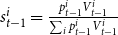 ${s}_{t-1}^{i}=\frac{{p}_{t-1}^{i}{V}_{t-1}^{i}}{\sum _{i}{p}_{t-1}^{i}{V}_{t-1}^{i}}$
is the product of sector
 $i$
share of aggregate real value added with sector
 $i$
price at
 $t-1$
. By rearranging Eq. (2) we can obtain:
 \begin{align} &g(X_{t})\nonumber\\[5pt] &\quad=\underset{\textit{Within } \textit{contribution}}{\underbrace{\sum _{i}{s}_{t-1}^{i}g({X}_{t}^{i})}}+\underset{\textit{Price } \textit{Gcontribution}}{\underbrace{\sum _{i}{s}_{t-1}^{i}g({p}_{t}^{i})}}+\underset{\textit{Labour } \textit{contribution}}{\underbrace{\sum _{i}{s}_{t-1}^{i}g({l}_{t}^{i})}}\nonumber\\[5pt]&\quad+\underset{\textit{Sum of Interaction } \textit{terms}}{\underbrace{\sum _{i}{s}_{t-1}^{i}g\!\left({X}_{t}^{i}\right)g\!\left({p}_{t}^{i}\right)+\sum _{i}{s}_{t-1}^{i}g\!\left({X}_{t}^{i}\right)g\!\left({l}_{t}^{i}\right)+\sum _{i}{s}_{t-1}^{i}g\!\left({l}_{t}^{i}\right)g\!\left({p}_{t}^{i}\right)+\sum _{i}{s}_{t-1}^{i}g({X}_{t}^{i})g\!\left({p}_{t}^{i}\right)g({l}_{t}^{i})}}\end{align}
Eq. (3) expresses the aggregate percentage growth rate of labour productivity decomposed into four components. The first component
 ${s}_{t-1}^{i}g({X}_{t}^{i})$
is the contribution of ‘within’ labour productivity growth in sector
 $i$
. The second
 ${s}_{t-1}^{i}g({p}_{t}^{i})$
is the contribution of relative price changes between sectors.Footnote
13
The third
 ${s}_{t-1}^{i}g({l}_{t}^{i})$
captures labour input reallocation. The last component consists of four interaction terms. The weights are the sector shares of aggregate nominal value added.
Although Eq. (3) highlights the price contribution to weighted ARPLP growth, a key limitation of this framework is that, as acknowledged in Diewert (Reference Diewert2016) and Calver and Murray (Reference Calver and Murray2016), aggregate productivity growth is influenced by changes in industries’ relative input and output prices, even when sectoral productivity levels and labour input shares remain constant. This challenges the common intuition that productivity growth is solely driven by technological factors (Reinsdorf, Reference Reinsdorf2015; Calver and Murray, Reference Calver and Murray2016). As noted by Tang and Wang (Reference Tang and Wang2015), relative output prices in real GDP measurement, captured in the chained-Fisher index, reflect dual roles—signalling value creation and capturing employment contribution through labour share. Disentangling price effects, however, offers a clearer lens for assessing pure labour productivity growth, which is often the focus of policymakers and analysts evaluating technological and efficiency changes.
To isolate relative price effects from intrinsic labour productivity growth, we construct a separate index of ARPLP whose weights move only with relative prices and labour-hours as follows:
 \begin{align}g\!\left(ALP_{t}\right)&=g\!\left(\mathrm{X}_{t}\right)-\sum _{i}{s}_{t-1}^{i}g\!\left({P}_{t}^{i}\right)-\frac{1}{2}\sum _{i}{s}_{t-1}^{i}g\!\left({X}_{t}^{i}\right)g\!\left({p}_{t}^{i}\right)-\frac{1}{2}{s}_{t-1}^{i}g\!\left({l}_{t}^{i}\right)g\!\left({p}_{t}^{i}\right)\nonumber\\&\quad -\frac{1}{3}\sum _{i}{s}_{t-1}^{i}g\!\left({X}_{t}^{i}\right)g\!\left({l}_{t}^{i}\right)g\!\left({p}_{t}^{i}\right)\nonumber\\&=\sum _{i}{s}_{t-1}^{i}g\!\left({X}_{t}^{i}\right)+\frac{1}{2}\sum _{i}{s}_{t-1}^{i}g\!\left({l}_{t}^{i}\right)g\!\left({X}_{t}^{i}\right)+\frac{1}{2}\sum _{i}{s}_{t-1}^{i}g\!\left({p}_{t}^{i}\right)g\!\left({X}_{t}^{i}\right)+\sum _{i}{s}_{t-1}^{i}g\!\left({l}_{t}^{i}\right)\nonumber\\&\quad+\frac{1}{2}\sum _{i}{s}_{t-1}^{i}g\!\left({l}_{t}^{i}\right)g\!\left({X}_{t}^{i}\right)+\frac{1}{2}\sum _{i}{s}_{t-1}^{i}g\!\left({l}_{t}^{i}\right)g\!\left({p}_{t}^{i}\right)+\frac{2}{3}\sum _{i}{s}_{t-1}^{i}g\!\left({X}_{t}^{i}\right)g\!\left({l}_{t}^{i}\right)g\!\left({p}_{t}^{i}\right)\end{align}
Hence, we haveFootnote 14
 \begin{equation}g\!\left(ALP_{t}\right)=\underset{\textbf{ARPLP}\text{ Growth}}{\underbrace{g\!\left(\mathrm{X}_{t}\right)}}-\underset{\boldsymbol{Relative} \, \boldsymbol{Price} \, \textit{Growth}}{\underbrace{g\!\left(AP_{t}\right)}}\end{equation}
where
 \begin{align}g\!\left(AP_{t}\right)& =\sum _{i}{s}_{t-1}^{i}g\!\left({P}_{t}^{i}\right)+\frac{1}{2}\sum _{i}{s}_{t-1}^{i}g\!\left({X}_{t}^{i}\right)g\!\left({p}_{t}^{i}\right)+\frac{1}{2}{s}_{t-1}^{i}g\!\left({l}_{t}^{i}\right)g\!\left({p}_{t}^{i}\right)\nonumber\\&\quad +\frac{1}{3}\sum _{i}{s}_{t-1}^{i}g\!\left({X}_{t}^{i}\right)g\!\left({l}_{t}^{i}\right)g\!\left({p}_{t}^{i}\right),\end{align}
Here we define aggregate relative price growth,
 $g(AP_{t})$
, as consisting of the sum of relative price changes and three interaction terms with labour hours and real value added per hour. The first term on the right-hand side of Eq. (5) is then the relative price and labour hours-weighted productivity growth (i.e., the ARPLP as defined previously). This rearrangement allows us to isolate the contribution of relative price changes from ALP, though not entirely because prices still remain inside the changing value-added weights. This nevertheless provides us a conceptual and methodological advance given that in Diewert (Reference Diewert2016) price growth and labour-share growth are combined multiplicatively and enter the weights.
By so doing, as shown in Eqs. (4) and (5), we can clarify more clearly the role of relative price movements, demonstrating how the economy-wide ALP growth rate is influenced by relative price changes, and makes transparent the channels through which price effects operate. Specifically, if the relative price for sector
 $i$
’s output increases sufficiently, it will contribute negatively to ALP growth; conversely, a significant decrease in relative price will result in a positive price contribution to ALP growth.Footnote
15
While Eq. (5) is informative about the relative price contribution to labour productivity growth, it remains, still, difficult to interpret because of the use of weights (and also interaction terms) that themselves still involve relative prices. Since it is clear that the GEAD cannot, even with our extension, cleanly isolate price effects, we turn to implement an extended T
 $\ddot{o}$
rnqvist decomposition to isolate the price contribution to ALP growth. We extend the framework by decomposing the ‘within’ component into three terms, Nominal VA Growth, Price Growth, and Labour Growth. We do so by expressing nominal value added per hour as follows:
 \begin{align*}\varDelta \textit{ ln}\! \left(V/L\right)&=\sum _{j}[0.5(w_{j,t}+w_{j,t-1})]\varDelta \textit{ ln} (V_{j}/L_{j})+\sum _{j}[0.5(w_{j,t}+w_{j,t-1})]\varDelta \textit{ ln} \bigg(L_{j}/\sum _{j}L_{j}\bigg)\\&=\sum _{j}\overline{w}_{j}\varDelta \textit{ ln} (V_{j}/L_{j})+\sum _{j}\overline{w}_{j}\varDelta \textit{ ln} \bigg(L_{j}/\sum _{j}L_{j}\bigg)\end{align*}
 \begin{align} &=\sum _{j}\overline{w}_{j}\left[\varDelta \textit{ ln}\! \left(\frac{NV_{j}}{P_{j}}\times \frac{1}{L_{j}}\right)\right]+R\nonumber\\ &=\sum _{j}\overline{w}_{j}[\varDelta (\textit{ ln } NV_{j}-ln P_{j}-ln L_{j})]+R\nonumber\\ &=\underset{\textit{Nominal } \textit{Growth}}{\underbrace{\sum _{j}\overline{w}_{j}\varDelta \textit{ ln } NV_{j}}}-\underset{\textit{Price } \textit{Growth}}{\underbrace{\sum _{j}\overline{w}_{j}\varDelta \textit{ ln } P_{j}}}-\underset{\textit{Labour } \textit{Growth }}{\underbrace{\sum _{j}\overline{w}_{j}\varDelta \textit{ ln } L_{j}+}}\underset{\textit{Labour } \textit{Reallocation}}{\underbrace{R}}\end{align}
where the change in
 $V$
is the weighted aggregate of changes in real industry value-added
 $V_{j}$
and weights
 $\overline{w}_{j}$
are shares of nominal value-added, averaged over two periods to form a T
 $\ddot{o}$
rnqvist index. We can now define the ALP growth decomposition (in logs) as:
 \begin{equation}\varDelta \textit{ ln}\! \left(V/L\right)=\sum _{j}\overline{w}_{j}\varDelta \textit{ ln } NV_{j}-\sum _{j}\overline{w}_{j}\varDelta \textit{ ln } P_{j}-\sum _{j}\overline{w}_{j}\varDelta \textit{ ln } L_{j}+R\end{equation}
Note that this decomposition framework has the advantage that it allows value-added functions (nominal share-weighted real value added for all industries) and output prices to differ across sectors (also see, Goodridge et al. Reference Goodridge, Haskel and Wallis2018; Goodridge and Haskel, Reference Goodridge and Haskel2023). In what follows, we will compare the two decompositions and apply them to both current double deflated and counterfactual single deflated data.
4. Data
Building on Coyle and Mei (Reference Coyle and Mei2023), we use Office for National Statistics (ONS)’s sectoral and division level data on nominal value added, real value added, and labour input (total hours worked).
For the sectoral level data, ONS provides Standard Industrial Classification 2007 (SIC07), dividing the whole UK economy into 20 (A-T) sectors.Footnote 16 A division in the manufacturing sector is, for instance, manufacture of food products, beverages and tobacco (CA 10–12), manufacture of textiles, wearing apparel and leather products (CB 13–15), manufacture of wood and paper products, and printing (CC 16–18), etc.Footnote 17
Prices at the sector-level are implied by the nominal and real value-added series. For real value added, we use the double deflated data for the UK, first introduced in October 2021, provided by the ONS. We also collected the previous single deflated real value-added data for the UK from the ONS national accounts dataset published prior to October 2021. Note that all real value-added series used in this paper are ONS chained-volume measures. Sector-level real GVA is constructed using chain-linked Fisher volume indices, hence the corresponding sectoral deflators
 ${P}_{t}^{i}$
and the aggregate deflator
 $P_{t}$
are therefore implicit Fisher-type deflators derived as nominal GVA divided by chained-volume GVA.Footnote
18
Note that our measure of labour input, as measured in total hours worked, does not incorporate labour heterogeneity, for example, differences in education, occupation, skills, or employment type. Although labour-quality-adjusted hours would be preferable in principle, such data are not available at the level of sectoral detail required for our sector-level decomposition.Footnote 19 Consistent with Coyle and Mei (Reference Coyle and Mei2023) and Goodridge and Haskel (Reference Goodridge and Haskel2023), we follow standard practice in sector-level productivity analysis by treating hours as homogeneous. While changes in labour composition could, in principle, influence the labour-input component of the decomposition, the contribution of relative prices—our main focus—is unlikely to be materially affected by labour heterogeneity; the price term reflects the behaviour of sectoral deflators rather than shifts in labour composition.
To assess firms’ market power, we follow Coyle et al. (Reference Coyle, McHale, Bournakis and Mei2024, Reference Coyle, McHale, Bournakis and Mei2026) and Coyle et al. (Reference Coyle, McHale, Bournakis and Mei2026) and use the firm-level dataset from the ONS Annual Business Survey (ABS), which covers non-financial businesses in the UK over 2008-2019. Consistent with standard practice, we apply the 2-digit industry-level ONS producer output price deflatorFootnote 20 and input price indices (manufacturing Producer Price Index (PPI) and non-manufacturing Services PPI)Footnote 21 to convert all nominal variables into 2015 prices (in £ thousands). Capital stocks are constructed using the Perpetual Inventory Method (PIM), following Coyle et al. (Reference Coyle, McHale, Bournakis and Mei2024, Reference Coyle, McHale, Bournakis and Mei2026) and Coyle et al. (Reference Coyle, McHale, Bournakis and Mei2026).Footnote 22 The analysis is conducted at the lowest local unit level, drawing on information on total revenue, wages, capital stock, and purchases of intermediates to estimate aggregate markups. To ensure consistency with the sector-level results, we focus on firms in the manufacturing and ICT sectors. This yields an unbalanced panel of 140,312 observations for manufacturing and 116,030 observations for ICT.
5. Results
5.1 Aggregate UK results
To contextualise the comparison between “value creation” price effects and the labour contribution to ALP growth, we first demonstrate the sensitivity of the ARPLP growth pattern to relative prices by presenting results for both single- and double-deflated data.Footnote 23 In doing so, we treat the earlier single-deflated real value-added series as a counterfactual benchmark because it represents the labour productivity path that would have been recorded had the ONS not adopted double deflation; prior to the 2021 introduction of double deflation, the ONS applied a single output deflator to both outputs and intermediate inputs, implicitly assuming that input and output prices moved identically. By contrast, double deflation separately deflates outputs and intermediate inputs and therefore allows divergences between input and output price movements to affect measured real value added. Comparing the two series thus enables us to isolate the extent to which measured labour-productivity dynamics—and in particular the relative-price component—are driven by economic forces (true input–output price divergence) versus measurement conventions embedded in the former single-deflation methodology. As we show below, this methodological distinction has important implications for the extended decomposition frameworks we employ.
Whole economy aggregate relative price labour productivity (ARPLP) growth 1998–2019.
Notes: ARPLP growth calculated using Eq. (2).

Figure 2 illustrates how the 20-sector aggregated ARPLP, which is the labour productivity decomposition used by the UK ONS,Footnote 24 varies between the single and double deflated data. The two series differ, sometimes substantially, while both trending down. Figure 3 then shows the Extended GEAD decomposition of ARPLP growth into its components. The relative price effect (red bar) is larger using double deflated data (on the left panel), particularly pre-2008 when it generally makes a positive contribution, whereas in the counterfactual data the ‘within’ component stands out (on the right panel). Thus, decomposition of the aggregated productivity growth rates is indeed sensitive to changes in relative input and output prices.
Whole economy aggregate relative price labour productivity growth (ARPLP) components, extended GEAD, 1998–2019.
Note: ARPLP growth decomposed using Eq. (3).

Recall that this ARPLP productivity growth measure can grow even if all industries’ productivity levels and labour input shares remain unchanged. These findings reinforce the point made in Coyle and Mei (Reference Coyle and Mei2023)Footnote 25 that the switch from single to double deflated data has had a significant impact on the labour productivity measure; the differences between input and output prices are captured by the differences in relative price contribution (red bars) between the two panels in Figure 3.
While treating a change in the input prices that an industry pays, or in the output price that it receives, as a contribution to aggregate productivity growth in itself is, as noted, at odds with the traditional intuition about the technological drivers of productivity growth, an appropriate price deflator may still allow the ARPLP to capture movement in the production possibility frontier caused by improvements in technology, that is, the ‘true’ difference between the change in the quantity of output and inputs. However, constructing such a ‘perfect’ price deflator is difficult because the selection of weights can greatly affect the index, especially when the economy is changing (e.g., Abdirahman et al. Reference Abdirahman, Coyle, Heys and Stewart2020, Reference Abdirahman, Coyle, Heys and Stewart2022).
Figure 4 (left) illustrates that aggregate ALP growth across the 20 sectors comprising the whole economy, as calculated using the extended T
 $\ddot{o}$
rnqvist framework, is broadly consistent between single-deflated (dashed line) and double-deflated (solid line) data, although a gap persists. In contrast, under the extended GEAD framework (Figure 4, right), the gap between double-deflated current data (solid line) and counterfactual older data (dashed line) is notably larger, particularly in the period before 2008. Furthermore, while both decompositions yield similar results when applied to single-deflated data (dashed lines), they diverge considerably when double-deflated data is employed (solid lines). Notably, the T
 $\ddot{o}$
rnqvist framework exhibits greater consistency between single- and double-deflated data, suggesting it is less sensitive to changes in input prices.Footnote
26
Whole economy aggregate labour productivity (ALP) growth 1998–2019.
Notes: labour productivity growth rates for 20 industries.

While both decomposition frameworks are theoretically valid and implemented consistently, the magnitude of the relative-price component differs across the extended GEAD and extended T
 $\ddot{o}$
rnqvist methods when double-deflated data is employed. This divergence reflects differences in accounting structure; in the extended GEAD framework, relative prices enter not only the price term itself but also the sectoral weights and several interaction terms, that is, the extended GEAD obtains ALP indirectly via ARPLP and relative-price-based weights. This is shown in Eq. (4), where the relative price term partially contributes to ALP growth as "value creation" through its interaction with within-sector (the third term in Eq. 4,
 $\frac{1}{2}\sum _{i}{s}_{t-1}^{i}g\!\left({p}_{t}^{i}\right)g\!\left({X}_{t}^{i}\right)$
) and labour (the sixth term in Eq. 4,
 $\frac{1}{2}\sum _{i}{s}_{t-1}^{i}g\!\left({l}_{t}^{i}\right)g\!\left({p}_{t}^{i}\right)$
) contributions. As a result, the extended GEAD is highly sensitive to differences between input and output deflation, which amplifies relative-price effects when double-deflated data are used. By contrast, the extended T
 $\ddot{o}$
rnqvist decomposition explicitly separates nominal value-added growth, price growth, and hours growth directly from the labour contribution, that is, it constructs ALP directly from log-changes in nominal value added, output prices, and hours using symmetric T
 $\ddot{o}$
rnqvist weights, and is therefore not affected by changes in deflator methodology. This feature likely accounts for the T
 $\ddot{o}$
rnqvist framework’s greater consistency and its robustness to the impact of input price changes.
While the comparison of the two approaches thus illustrates that part of the observed variation in the GEAD price component reflects methodological decisions, it is worth emphasising that although the extended GEAD and extended T
 $\ddot{o}$
rnqvist decompositions yield different aggregate levels of ALP growth in Figure 4 when double-deflated data is employed, the overall patterns, including the timing of peaks, troughs, and broad cycles, remain remarkably similar. As a result, these levels do not coincide, but the similar dynamics across methods indicate that both decompositions capture consistent macroeconomic movements in UK productivity.
Figures 5 and 6 present the decompositions using double-deflated data exclusively. Figure 5 illustrates aggregated ALP growth (white dots) calculated using the extended T
 $\ddot{o}$
rnqvist decomposition (Eq. 8), while Figure 6 depicts aggregated ARPLP growth (white dots) derived from the extended GEAD framework (Eq. 5).
UK labour productivity growth extended T
 $\ddot{o}$
rnqvist decomposition.
Notes: White dots show the whole economy labour productivity growth rate, blue for nominal value added growth, red for price change, grey for total hours worked growth, and black for the reallocation. Both price and hours increase in absolute terms, over time; negative terms are subtracted from the nominal growth rate in order to obtain the labour productivity measure.

UK labour productivity growth, extended GEAD decomposition.
Notes: White dot for whole economy labour productivity growth rates, blue for aggregate relative price labour productivity growth and red for relative price growth. Negative terms are subtracted from the ARPLP growth to obtain labour productivity.

Our results reveal that relative price changes (red bars in Figures 5 and 6) and hours worked (grey bars in Figure 5) negatively contribute to ALP growth. In both the extended T
 $\ddot{o}$
rnqvist and extended GEAD frameworks, the magnitude of the price contribution declines over time, partially offsetting the post-2008 productivity slowdown. Simultaneously, the nominal gross value-added component (blue bars) also diminishes after 2008. The labour reallocation term, however, remains relatively small throughout the period. Moreover, the aggregated ARPLP growth pattern (white dots) in Figure 6 during the pre-2008 period closely resembles the ALP growth pattern in Figure 5 once the relative price contribution is subtracted from ALP growth (white square dots).
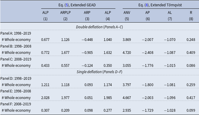
Table 1 presents the detailed aggregated ALP growth rates, with columns 1-3 showing results from the extended GEAD decomposition and columns 4-8 from the extended T
 $\ddot{o}$
rnqvist decomposition. Panels A to C display results based on the current double-deflated data, while Panels D to F present the results based on the counterfactual single-deflated data. As previously noted, the extended GEAD decomposition differs considerably between the current and counterfactual datasets. In contrast, the preferred extended T
 $\ddot{o}$
rnqvist decomposition shows more consistency between the two datasets.
Labour productivity growth 1998–2019

Table 1. Long description
A table comparing labour productivity growth rates using different decomposition methods and data sets. The table has 8 columns and 6 rows, including headers and panel labels. Columns are labeled as ALP, ARPLP, ARP, ALP, ANV, AP, AL, and R. Rows are grouped into Panels A to F, each representing different time periods and data deflation methods. Panel A: 1998-2019, Whole economy: 0.677, 1.126, -0.448, 1.040, 3.869, -2.007, -1.070, 0.248. Panel B: 1998-2008, Whole economy: 0.772, 1.677, -0.905, 1.632, 4.720, -2.408, -1.087, 0.409. Panel C: 2008-2019, Whole economy: 0.433, 0.557, -0.124, 0.350, 3.055, -1.776, -1.015, 0.086. Panel D: 1998-2019, Whole economy: 1.211, 1.118, 0.093, 1.174, 3.797, -1.800, -1.081, 0.259. Panel E: 1998-2008, Whole economy: 2.028, 1.977, 0.051, 1.985, 4.667, -2.003, -1.096, 0.417. Panel F: 2008-2019, Whole economy: 0.307, 0.209, 0.098, 0.277, 2.935, -1.729, -1.028, 0.099.
Notes: Data are average growth rates per year for 1998–2019. Sum columns (2) to (3) equal to column (1) for each row, subject to rounding. Sum columns (4) to (8) equal to column (4) for each row, subject to rounding. For columns (1) to (3), ALP refers to aggregate labour productivity growth, ARPLP refers to aggregate relative price labour productivity growth, ARP refers to aggregate relative prices growth. For columns (4) to (8) then, ALP is aggregate labour productivity growth, ANV is aggregate nominal gross value growth, AP is aggregate prices growth, AL is aggregate hours growth, and R is the reallocation.
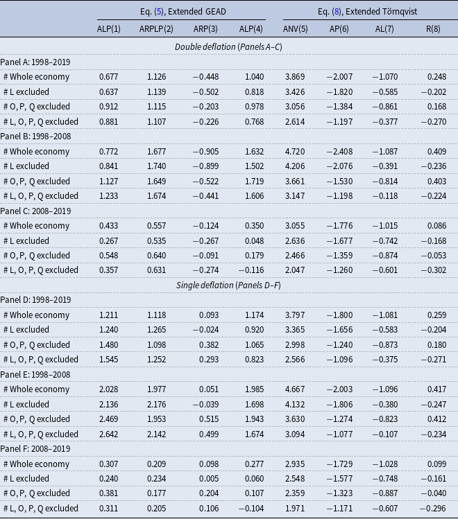
Following Coyle and Mei (Reference Coyle and Mei2023) and Goodridge and Haskel (Reference Goodridge and Haskel2023), Table 2 presents results when industry sectors such as real estate activities (labelled as L), public administration (labelled as O), education (labelled as P), and human health (labelled as Q) are excluded, respectively. We also include results where sectors L, O, P, and Q are simultaneously excluded.Footnote 27 As shown, the aggregate productivity decomposition is significantly affected by the exclusion of real estate and non-market sectors, pointing to the need to explore further price and volume measurement in these cases where the measurement issues are challenging.
Labour productivity growth 1998–2019

Table 2. Long description
The table presents labour productivity growth data from 1998 to 2019, focusing on the impact of excluding specific industry sectors. It includes results for the whole economy and scenarios where sectors like real estate, public administration, education, and human health are excluded. The table is divided into panels A to F, each showing different combinations of excluded sectors and deflation methods. Each panel includes columns for various productivity metrics and rows for different time periods and exclusion scenarios. Panel A covers 1998-2019 with double deflation, Panel B covers 1998-2008 with double deflation, Panel C covers 2008-2019 with double deflation, Panel D covers 1998-2019 with single deflation, Panel E covers 1998-2008 with single deflation, and Panel F covers 2008-2019 with single deflation. Each row lists specific productivity metrics and their values under different scenarios.
Notes: Data are average growth rates per year for 1998–2019. Industry L is real estate activities, O is public administration, P is Education, and Q is human health. Sum columns (2) to (3) equal to column (1) for each row, subject to rounding. Sum columns (4) to (8) equal to column (4) for each row, subject to rounding. For columns (1) to (3), ALP refers to aggregate labour productivity growth, ARPLP refers to aggregate relative price labour productivity growth, ARP refers to aggregate relative prices growth. For columns (4) to (8) then, ALP is aggregate labour productivity growth, ANV is aggregate nominal gross value growth, AP is aggregate prices growth, AL is aggregate hours growth, and R is the reallocation.
5.2. Manufacturing and ICT
Coyle and Mei (Reference Coyle and Mei2023) showed that a small number of high-value sectors, manufacturing and ICT accounted for the largest contributions to the UK labour productivity growth slowdown after 2008 (see Figure 7). Here we disaggregate the data to the ONS division level to investigate how the relative price effects under the two alternative decomposition approaches affect ALP growth patterns (and hence the slowdown) in these two sectors. We define the ALP growth for manufacturing and ICT, respectively, as follows:
 \begin{equation}g\big({ALP}_{t}^{\,j}\big)=g\big({X}_{t}^{j}\big)-g({AP}_{t}^{j})\end{equation}
and
 \begin{equation}\textit{ln } \big(V_{j}/L_{j}\big)=\sum _{n}\overline{w}_{n}\varDelta \textit{ ln } NV_{n}-\sum _{n}\overline{w}_{n}\varDelta \textit{ ln } P_{n}-\sum _{n}\overline{w}_{n}\varDelta \textit{ ln } L_{n}+R_{j}\end{equation}
where
 $g({X}_{t}^{j})$
is again the ARPLP growth (i.e., between times
 $t$
and
 $t-1$
as defined before) of sector
 $j$
,
 $g({AP}_{t}^{j})$
refers to sector
 $j$
’s aggregate price growth consisting of the sum of relative price changes and three interaction terms with labour hours and real value added per hour,
 $\varDelta \textit{ ln } NV_{n}$
,
 $\varDelta \textit{ ln }P_{n}$
, and
 $\varDelta \textit{ ln} L_{n}$
refer to nominal growth, price growth, and labour growth of subsector
 $n$
within sector
 $j$
, R is the reallocation, weights
 $\overline{w}_{n}$
are shares of nominal value-added averaged over two periods to form a T
 $\ddot{o}$
rnqvist index, and superscript
 $n$
refers to each ONS division within sector
 $j $
(i.e.,
 $n=10, 11,\ldots , 18$
for manufacturing, and
 $n=34, 35,\ldots , 39$
for ICT).
The slow growth of labour productivity—Manufacturing and ICT.
Notes: We calculate the average growth rate of labour productivity using the Tornqvist approach adopted by Coyle and Mei (Reference Coyle and Mei2023). Panel A presents the growth rate over time, while Panel B shows the average growth patterns for the periods 1998–2008 and 2009–2019. In Panel B, the light blue chart represents the average growth rate of labour productivity in manufacturing for 1998–2008, the rose chart for manufacturing in 2009–2019, the green chart for ICT in 1998–2008, and the grey chart for ICT in 2009–2019.

Figure 7. Long description
Panel A: A line graph shows the growth rate of labor productivity over time from 1998 to 2019. The y-axis represents the labor productivity growth rate in percent, ranging from 0 to 25 percent. The x-axis represents the years from 1998 to 2019. Two lines are plotted: one for manufacturing in light blue and one for ICT in green. The manufacturing line shows a general decline over the years, while the ICT line exhibits more fluctuations with peaks and troughs. Panel B: A bar graph compares the average growth rate of labor productivity over two periods: 1998-2008 and 2009-2019. The y-axis represents the labor productivity growth rate in percent, ranging from 0 to 12 percent. The x-axis has four categories: M98-07, M08-19, ICT98-07, and ICT08-19. The light blue bar represents manufacturing from 1998-2008, the rose bar represents manufacturing from 2009-2019, the green bar represents ICT from 1998-2008, and the grey bar represents ICT from 2009-2019. The green bar for ICT98-07 is the highest, indicating the highest average growth rate, while the rose bar for M08-19 is the lowest.
Figures 8 and 9 plot growth rates (white dots) and the contribution of each growth component over time for the Extended GEAD (Eq. 9) and Extended T
 $\ddot{o}$
rnqvist (Eq. 10) decompositions respectively. Each adopts both double deflated and single deflated (counterfactual) data. As before, the extended GEAD framework (Figure 8) is substantially affected by double deflation in both sectors. By contrast, the extended T
 $\ddot{o}$
rnqvist approach (Figure 9) provides broadly more consistent results.
Cumulative labour productivity growth (Extended GEAD).
Notes: White dot for sector labour productivity growth rates, blue chart for aggregate relative price labour productivity growth and red for relative price growth. Price growth should be interpreted in absolute term, that is, price term grows overtime. Negative terms are subtracted from the ARPLP growth in order to obtain the labour productivity measure ALP.

Cumulative labour productivity growth (Extended T
 $\ddot{o}$
rnqvist).
Notes: White dots for sector labour productivity growth rates, blue for nominal value-added growth, red for relative price change, grey for total hours worked growth, and black for the reallocation. Both price and hours increase in absolute terms over time; negative terms are subtracted from the nominal growth rate in order to obtain the labour productivity measure ALP.

Figure 9. Long description
Panel A Double Deflation: Two bar graphs compare growth rates in manufacturing and ICT sectors. The x-axis represents years from 1998 to 2019, and the y-axis represents the growth rate in percent. The graphs use different colors to represent nominal growth (blue), price growth (red), labor growth (grey), and reallocation (black). Panel B Counterfactual (Single) Deflation: Two bar graphs compare growth rates in manufacturing and ICT sectors using single deflation. The x-axis represents years from 1998 to 2019, and the y-axis represents the growth rate in percent. The graphs use different colors to represent nominal growth (blue), price growth (red), labor growth (grey), and reallocation (black).
When comparing the results for both sectors in Figures 8 and 9 under the two decompositions, the differences are striking. The price effects in the case of ICT vary significantly between single and double deflated data using the Extended GEAD, although this variation is less pronounced when using the extended T
 $\ddot{o}$
rnqvist method. Specifically, with extended GEAD (Figure 8), the price contribution becomes positive in many years when using single-deflated data, but the ARPLP term (blue bars) becomes substantially smaller, leading to a lower overall growth rate for ICT. The slowdown is even more pronounced when double-deflated data is used. While the extended T
 $\ddot{o}$
rnqvist approach shows a more consistent slowdown pattern regardless of the dataset, the price contribution behaves differently: it is more consistently positive and exhibits less slowdown in the actual data compared to the counterfactual. Nonetheless, the growth patterns of ICT’s ALP (represented by the white dot) and price contributions are significantly different when analysed with double versus single deflator data, assuming all other factors remain constant. With double-deflated data, we consistently observe positive price contributions to ALP growth, whereas single-deflated data shows little effect, except in 1999, 2000, and 2001, when positive contributions to ALP growth are observed.Footnote
28
6. Markups and market power?
The large differences in the price component across decomposition methods, and its substantial contribution to ALP growth, are striking. As noted by Diewert (Reference Diewert2016), one would expect the effect of relative price changes to be small; because the aggregate deflator reflects industry prices, an increase in one industry’s relative price should be offset by a decline elsewhere, implying that relative price contributions should approximately sum to zero. In practice, however, the overall impact can be more complex. Using cross-country data, Dumagan (Reference Dumagan2013b) and Dumagan and Balk (Reference Dumagan and Balk2016) show that relative price changes rarely sum to zero and can affect both reallocation effects and sectoral contributions to ALP.
Consistent with these findings, in Section 5 we demonstrate that relative price movements are far from negligible. At the aggregate level (Section 5.1), relative prices contribute between negative
 $1$
and negative
 $2$
percentage points per year to ALP growth. At the sectoral level (Section 5.2), the price component is particularly large and volatile in ICT. This raises the question of what structural forces might account for such substantial and asymmetric price effects.
A natural explanation lies in the evolution of market power. A large literature documents significant changes in market structure-including the rise of “superstar” firms, increases in markups, and declining business dynamism (De Loecker et al. Reference De Loecker, Eeckhout and Unger2020; Autor et al. Reference Autor, Dorn, Katz, Patterson and Van Reenen2020). When markups vary over time, sectoral output prices may diverge from the aggregate deflator, generating persistent relative price movements. From this perspective, the UK aggregate output price deflator increases steadily over 1998-2019 under both single and double deflation (Figure 10). The pronounced divergence between the single- and double-deflated series may also reflect underlying changes in measurement methodology and shifts in firms’ cost structures, including potential changes in market power. This suggests that shifts in market power may have contributed to the substantial relative price effects observed in Section 5.
Price evolution 1998–2019.
Notes: This figure plots the overall price (deflator) evolution overtime 1998–2019 double (blue) versus single (red). Whole economy price deflator for 20 industries. 1998 is rebased to 1.
Source: ONS and Authors’ calculations.

Our results show that the price effect is large and highly variable in ICT but relatively small in manufacturing. We hypothesise that both sectors exhibit meaningful variation in markups over time and that such variation may represent an important source of relative price movements. To test this mechanism, we adopt the production-approach estimator, where markups are derived from the first-order conditions (FOCs) of a cost-minimising firm with at least one flexible input in the presence of fixed costs (Hall, Reference Hall1988; De Loecker, Reference De Loecker2011; De Loecker and Warzynski, Reference De Loecker and Warzynski2012).
First, following Coyle et al. (Reference Coyle, McHale, Bournakis and Mei2024, Reference Coyle, McHale, Bournakis and Mei2026) and Coyle et al. (Reference Coyle, McHale, Bournakis and Mei2026), we employ ONS ABS firm-level data for the period 2008–2019. We focus on the manufacturing and ICT sectors, as these sectors were consistently identified as important contributors in our sectoral-level analysis. Second, following Hall (Reference Hall1988), De Loecker (Reference De Loecker2011), and De Loecker and Warzynski (Reference De Loecker and Warzynski2012), we start with a general production function
 $\mathrm{Q}_{\mathrm{it}}=\mathrm{F}(\mathrm{L}_{\mathrm{it}},\mathrm{K}_{\mathrm{it}},\mathrm{M}_{\mathrm{it}})$
,Footnote
29
and then use the Lagrangian for the cost-minimisation problem. With the FOC with respect to the variable materials input and multiplying both sides by
 $\mathrm{Q}_{\mathrm{it}}/\mathrm{M}_{\mathrm{it}}$
and using the definition of the (gross) markup as
 $u_{it}=\mathrm{P}_{\mathrm{it}}/{\unicode[Arial]{x03C7}} _{\text{it }}$
, we obtain
 \begin{equation}\mu _{it}=\beta _{it}\!\left(\alpha _{it}\right)^{-1}.\end{equation}
where
 $\beta _{it}$
is the elasticity of output with respect to the flexible input materials, and
 $\alpha _{it}$
is therefore the share of material expenditure in total firm revenue.Footnote
30
To obtain the output elasticities of input materials, we regress firm-level price-deflated revenue on labour input
 $l_{it}$
, capital input
 $k_{it}$
, and material input
 $m_{it}$
. The coefficient of the material input is then the elasticity of output with respect to the flexible input materials.Footnote
31
We then use firms’ market shares as weights to aggregate firm-level markups within each sector and construct a markup index, normalised to unity in the base year, for manufacturing and ICT.
Figure 11 presents the results. Both manufacturing and ICT exhibit substantial variation in markups over 2008–2019. In each sector, markups decline following the 2008–2009 global financial crisis, before rising notably during 2010–2015, by around one percentage point in manufacturing and about one percentage point in ICT. Overall, however, markups trend downward over the post-2008 period; declining by approximately four percentage points in ICT and by about two percentage points in manufacturing.
Revenue weighted markups index.
Notes: Markup estimates are based on ABS firm-level dataset spanning 2008–2019. There are 140,312 and 116,030 observations for manufacturing and ICT, respectively. We estimate a firm-level revenue function through each SIC4 sectors to get the elasticity substitution estimates and then calculate markups based on Eq. (11). We then apply revenue weights for each firm to get the aggregate markup level trend. The value of the index is set equal to 1 in 2008.

These findings are consistent with the sector-level results in Section 5, which show that price dynamics—and in particular the relative price contribution to ALP—are considerably more pronounced in ICT than in manufacturing. The markup estimates therefore provide a structural interpretation of the patterns revealed by the extended GEAD and T
 $\ddot{o}$
rnqvist decompositions. Sectors experiencing larger and more volatile changes in markups, notably ICT, are precisely those where we observe substantial and variable relative price effects in the decomposition results.
The mechanism is straightforward. A decline in markups reduces output prices relative to the aggregate deflator, thereby increasing real value added and generating a positive contribution to ALP growth, particularly under the T
 $\ddot{o}$
rnqvist framework where price changes are isolated cleanly. Hence, the secular decline in ICT markups over 2008–2019 aligns with the stronger positive price contributions observed in ICT. Conversely, periods of rising ICT markups—most prominently during 2010–2014—correspond to weaker or negative relative price contributions, consistent with the extended GEAD and T
 $\ddot{o}$
rnqvist results. Manufacturing, where markups change only modestly, correspondingly displays only small relative price effects.
With these consistent results, the decomposition exercise and markup analyses reveal a coherent and mutually reinforcing narrative. ICT’s larger relative price contribution to ALP growth reflects not only measurement differences arising from deflation methods but also underlying market-structure changes—most notably declining markups associated with rapid technological change, shifts in competitive pressure, and differences in input–output price dynamics. Manufacturing’s more muted markup fluctuations explain its more limited price-driven contributions, reinforcing the view that productivity dynamics in manufacturing are primarily driven by within-sector productivity growth rather than by relative prices or market-power effects.
Overall, the markup evidence deepens our understanding of the relative price component in the productivity decompositions. Rather than interpreting relative price effects solely as artefacts of deflator construction or quality adjustment, the results indicate that industry-level market power is an important mechanism shaping sectoral output prices and, thereby, measured labour productivity. This connection strengthens the broader of the paper; sector-specific market-structure dynamics, particularly in ICT, play a meaningful role in shaping the aggregate productivity record.
7. Discussion and conclusions
Existing studies that decompose ALP growth have largely overlooked the role of relative output price shifts between sectors. However, if these shifts are substantial, they can significantly influence the growth decomposition. In this paper, we address this gap by comparing the extended GEAD and T
 $\ddot{o}$
rnqvist approaches, applied to both double- and single-deflated UK data. This allows us to isolate the effects of sectoral relative output and input price changes from the more commonly examined within-sector and labour reallocation components of productivity decomposition.
Our analysis reveals that relative price components have a negative impact on ALP growth in both pre- and post-2008 periods. Specifically, under the extended GEAD framework, relative price shifts reduce ALP growth by 0.905 and 0.124 percentage points in the earlier and later periods, respectively. Similarly, the extended T
 $\ddot{o}$
rnqvist approach also indicates significantly negative contributions from relative price changes, particularly in the later period, with reductions of 2.408 and 1.776 percentage points for the earlier and later periods, respectively, using double-deflated data. At the division level, with a focus on the manufacturing and ICT sectors, we find that relative price effects are more pronounced in the ICT sector but remain relatively marginal in manufacturing.
What picture of the productivity dynamics in the economy can we take from this exercise? One possible explanation for our results could be market power and rising markups in the sectors of interest. There is now a large literature (De Loecker et al. Reference De Loecker, Eeckhout and Unger2020; Autor et al. Reference Autor, Dorn, Katz, Patterson and Van Reenen2020) on market power, finding evidence for the United States at least of higher markups at firm level, growing dominance of big companies (‘superstar’ firms), and declining business dynamism, for the whole economy. When overall relative price increases and assuming demand is inelastic, it implies that market power among firms in the industry is rising, hence firms within a particular industry can raise prices (Bräuning et al. Reference Bräuning, Fillat and Joaquim2022). To explore this further, we analyse UK firm-level data and consistently find evidence of significant variation in markups over time. These variations in markups are reflected in the substantial variations observed in price effects, reinforcing the notion that market power plays a critical role in shaping productivity dynamics.
In any case, while all decompositions are a series of snapshots of a dynamic phenomenon, by introducing the contribution of shifts in relative prices, this paper raises questions about how to interpret the effect of relative price changes in productivity dynamics. As discussed in Abdirahman et al. (Reference Abdirahman, Coyle, Heys and Stewart2020, Reference Abdirahman, Coyle, Heys and Stewart2022) in the context of telecommunications, it is challenging to ‘correctly’ assign economic value added or productivity when the alternative (volume or revenue) weights diverge—as they do during periods of relative price shifts—as the choice of nominal or real share weights will substantially affect the results. Similarly, Coyle and Hampton (Reference Coyle and Hampton2023) find that using a volume-based deflator (i.e., the cost per unit of computation as a basic unit for all products) in ICT produces price declines substantially larger than the official semiconductor PPI. The different decompositions embed different choices about using nominal and volume-based weights.
This issue is likely to arise in dynamic sectors such as ICT. Our results suggest that while the various decompositions consistently indicate that manufacturing and ICT both contribute significantly to the ALP growth slowdown in the UK post-2008, there are different phenomena in the two sectors. In manufacturing the ‘pure’ labour productivity (within and reallocation) elements are more prominent, consistently across decompositions and data sets. In ICT—consisting of computer software and services and telecommunications services—the relative price contributions we isolated play a larger part, and one that varies depending on method and data. This points to the need for further consideration of the measurement of quality adjusted input and output prices in this and other sectors experiencing technical or quality change.
Finally, our findings suggest that the extended T
 $\ddot{o}$
rnqvist framework provides a more appropriate framework for analysing relative price effects because it enables their complete isolation. By contrast, our theoretical analysis shows that complete isolation of relative price effects appears infeasible within the extended GEAD framework. Although the extended GEAD decomposition partially isolates relative price effects and offers additional insights into the sources of productivity growth, it remains sensitive to the choice between single and double deflation. Future research may therefore focus on developing aggregate productivity accounting frameworks that better isolate relative price effects while preserving the desirable properties of existing decomposition approaches.
Supplementary material
The supplementary material for this article can be found at https://doi.org/10.1017/S1365100526101436.
Acknowledgements
We thank the Editor, William Barnett, the Associate Editor, and two anonymous referees for their constructive and helpful comments and feedback on our manuscript. We are also grateful to Erwin Diewert, Peter Goodridge, Richard Heys, Bart Van Ark, Tony Venables, Dimitri Zenghelis, and Matthew Agarwala for their helpful comments on an early draft. We also thank all participants in a Productivity Institute workshop in Manchester in December 2022. Coyle is grateful for funding from the Productivity Institute, ESRC grant number ES/V002740/1, Mei for funding from the Gatsby Foundation and ONS research support grant number G116679/ONS2014988, and Hampton for funding from the Gatsby Foundation.








 o¨



 o¨


 Open access

