Introduction
Fermi Paradox has important scientific and science policy consequences. For example, how much money is it reasonable to spend on Search for Extraterrestrial Intelligence (SETI) projects? (Harp et al. Reference Harp2016) Simply stated, Fermi Paradox arises from a back-of-the-envelope calculation about how much time a technological civilization, able to perform interstellar colonization (colonizing civilizations or CCs for short), needs to diffuse through the entire Galaxy. With conservative assumptions, this calculation gives a colonization time of the order of a hundred million years (Hart Reference Hart1975; Crawford, Reference Crawford2000; Webb Reference Webb2015). Fermi Paradox can indeed be sharper because there is a possibility of intergalactic colonization (Armstrong & Sandberg Reference Armstrong and Sandberg2013).
It is important to notice that, for this conclusion to hold, we need not to assume any knowledge about the sociology of such civilizations, say, their continued desire to pursue with colonization efforts, etc. We need only to assume that, from all the CCs that emerged in the galactic history, which could be a large number, at least one succeed in creating a supercritical branching process where, at each time step, the number of new colonies plus the surviving ones is, in average, superior to the number of parent ones. However, since they clearly have not colonized us, we must necessarily conclude, says Fermi Paradox, that there is no such galactic spanning civilization: or there is no CCs, or all colonization clusters made by CCs are subcritical branching processes.
This scenario, however, is based on a hidden assumption: that the Solar system localization is typical, not exotic. However, typicality depends on the observer eyes. For example, we live in Brazil, and sometimes we wonder about strange places with curious behaviours of their inhabitants: sometimes they refer to football as soccer! Very exotic places, indeed.
However, we must recognize that there are also exotic places (and even whole populations) inside Brazil, which have never been contacted by the global civilization. Suppose that you are a member of a never visited Amazonian tribe. Now, it is obvious that a hypothetical technological civilization, able to perform air travel at 800 km h−1, certainly had time to colonize the entire Earth. However, since it has not reached you (remember, you are a member of an undiscovered Yanomami tribe), should you conclude, by using Fermi Paradox, that there is no such global civilization?
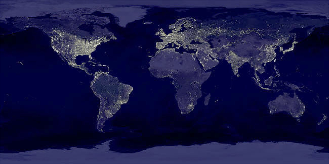
A nice view of the global civilization is given by the lights of the nocturnal Earth observed from the space (see Fig. 1). It is clear from this view not only the uneven distribution of global wealth but also the fact that the diffusion process of technology is highly non-uniform. Huge areas are not inhabited, and even never visited (or only visited by fanatic explorers). However, despite the provincial worldview of lost tribes, the global civilization is there.
Earth nocturnal lights suggest that several regions, of very different areas, are not colonized by the global technological civilization. Credit: Data courtesy Marc Imhoff of NASA GSFC and Christopher Elvidge of NOAA NGDC. Image by Craig Mayhew and Robert Simmon, NASA GSFC.
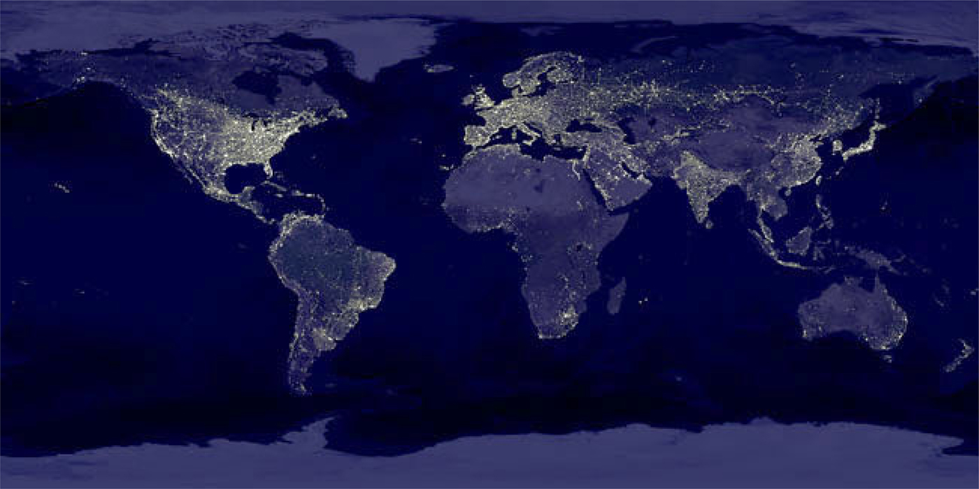
Human colonization clearly is not a simple and uniform diffusion process as assumed by a naive Fermi's calculation, but presents a hierarchical structure of empty regions of all sizes remembering a fractal cluster. Even a single city does not correspond to a compact cluster but presents fractal properties (Batty Reference Batty, Crilly, Earnshow and Jones1991).
Here we propose a generalized invasion percolation (GIP) process that interpolates between usual diffusion, which forms compact Eden clusters of colonized sites (Eden Reference Eden1961) and invasion percolation (IP), which forms fractal clusters (Wilkinson & Willemsen Reference Wilkinson and Willemsen1983; Sheppard et al. Reference Sheppard1999). The important new ingredient of our model, not present in standard IP, is that we can relate the time step of our algorithm to physical time, a crucial ingredient needed to explain Fermi Paradox. We also discuss why this generalized model is more realistic for the astronomical context than simple IP or the original percolation solution proposed by Landis (Landis Reference Landis1998; Webb Reference Webb2015).
We notice that a previous unpublished paper from one of us (Kinouchi, Reference Kinouchi2001, arXiv: cond-mat/0112137), with some percolation ideas to solve Fermi Paradox, has been cited by several authors including (Cirkovic Reference Cirkovic2003a, Reference Cirkovicb; Hetesi & Regaly Reference Hetesi and Regaly2006; Cirkovic Reference Cirkovic2009; Haqq-Misra & Baum Reference Haqq-Misra and Baum2009; Vukotic & Cirkovic Reference Vukotic and Cirkovic2012; Webb Reference Webb2015). However, although the general idea is correct, the specific (branching process) model presented in that paper is defective. Now we fix that problem with our new GIP colonization model.
The GIP model
The simulations are done in a square lattice with edge L = 100 that will represent a portion of the Galaxy (the relation with true astronomical size is discussed later). Our model is two-dimensional because to consider the thickness of the Galaxy will not change the main conclusions. Each site (i, j), i = 1, …, L; j = 1, …, L has a habitability barrier E ij∈[0, 1], which is an uniform random number generated and fixed from the start of the simulation (quenched disorder). This number intends to represent how hard it is to find a habitable planet in the unitary square with coordinates (i, j): the lower E ij, the easier to colonize that region. We discuss other choices for P(E ij) later.
Each site represents an area of D × D ly2 and can have two states: S ij = 0 (unoccupied) and S ij = 1 (colonized). We start with a single occupied site (the seed) at the centre of the lattice that represents a single mother civilization. Then, at the next time step, this civilization tries to colonize all its four nearest neighbours with indexes k = i ± 1, l = j ± 1 with probability P(S kl = 1) = p(E) = exp(−β E kl).
We continue this process with a parallel update where all occupied sites that have some unoccupied neighbour try to colonize them at each discrete time t. The time step between two colonization attempts is Δt. The time index t can be related to a physical timescale if we assign to Δt some plausible time interval comprising the time of a planet to be colonized, its development as a new CC and the time necessary for a colonizing mission to travel D light-years to the next empty region. Ideally, D must be related to the volume containing, on average, a single habitable stellar system to be colonized. We tentatively assume D = 10 ly. Since a time interval of 100 years seems to be very short and 10 000 years seems to be somewhat long, we choose the order of magnitude estimate Δt = 1000 years.
The lattice with (LD)2 ly2 represents a portion of space inside the galactic habitable zone (GHZ) in d = 2 dimensions (Lineweaver et al. Reference Lineweaver, Fenner and Gibson2004; Ramirez et al. Reference Ramirez2017). To compare our LD × LD simulations with the true area of the GHZ, we can approximate it by a rectangular strip of area H × B. The side H = R + − R − corresponds to the difference between the exterior R + and the interior radii R − of the GHZ zone, that is, the GHZ thickness. The side B = 2π (R + + R −)/2 = π (R + + R −) is related to the average perimeter of the GHZ, so the rectangle H × B has the same area of that the GHZ annulus. The standard values for the GHZ are R + = 10 kpc and R − = 4 kpc (Lineweaver et al. Reference Lineweaver, Fenner and Gibson2004), leading to H≈20 000 ly and B≈140 000 ly.
Due to computational limitations, we perform simulations in a square of area A = LD × LD = 106 ly2, which is small compared with H × B≈2,8 × 10⁹ ly2≈2, 800A. This occurs because simulation times grow exponentially for large β, preventing us to work with the lattices with the edges H and B (this is discussed later). However, we think that this fact is not relevant for our purposes, since for large β, the colonization cluster is approximately scale invariant (fractal-like), so that our main conclusions do not depend on scale. The scale invariance of our results is also robust if more recent data about the GHZ structure are used (Morrison & Gowanlock Reference Morrison and Gowanlock2015; Rossmo Reference Rossmo2017).
Notice that the invasion criteria based in the βE ij parameter mimics intelligent colonization, not simple diffusion: the exponential factor means that the sites first chosen to be colonized are those that have a lower barrier E ij, that is, high habitability. The free parameter β measures the average difficulty of the colonization process, aggregating, for example, the technological challenge of interstellar voyages and colony terraforming. We can interpret T = 1/β as the technological level of the civilization.
Results
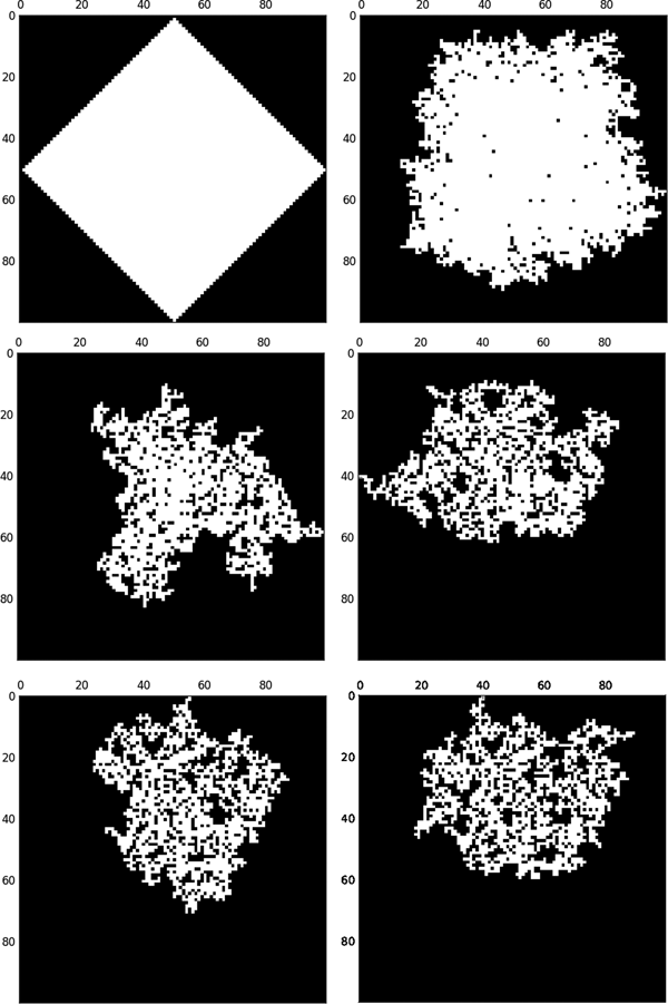
In Fig. 2, we show the instances of the colonization cluster from different difficulty parameters β. For β = 0, we have a deterministic colonization where all neighbours are colonized with probability one notwithstanding the value of E ij: the square geometry of the growing cluster is an artefact of the process symmetry.
From top to bottom, left to right, clusters with β = 0, 5, 10, 15, 20 and 25. The initial seed is at i = 50, j = 50 and the stop criteria is that the cluster touches some border.

For small β, we obtain compact clusters very similar to the Eden growth model (Eden Reference Eden1961). For larger β, the colonization clusters start to appear more fractal like. In particular, for β>15, large voids of uncolonized sites appear. Our proposal is that Earth is well inside of one of these voids that, in the full model with area H × B can be very large (due to the scale invariance of the voids sizes).
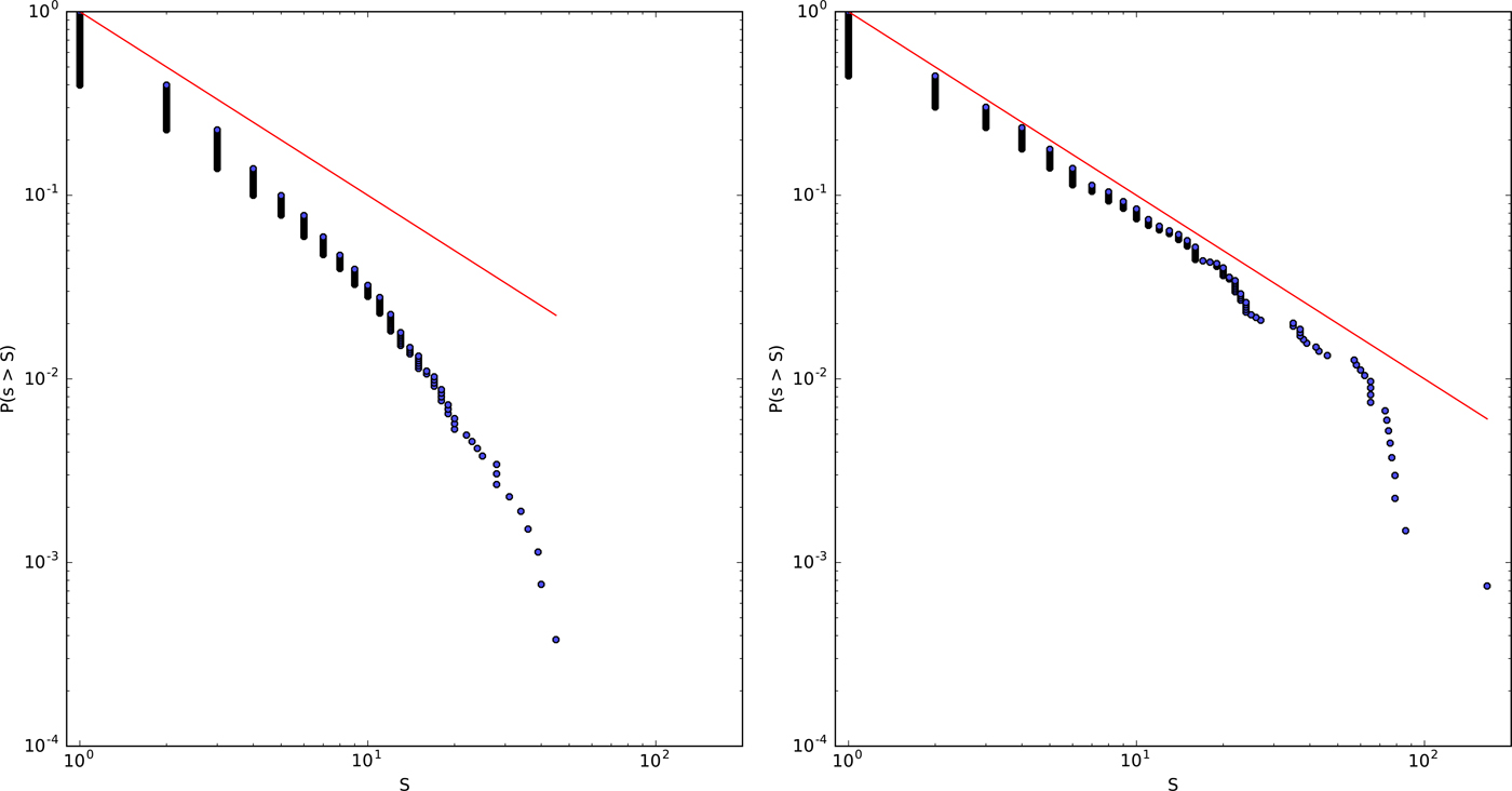
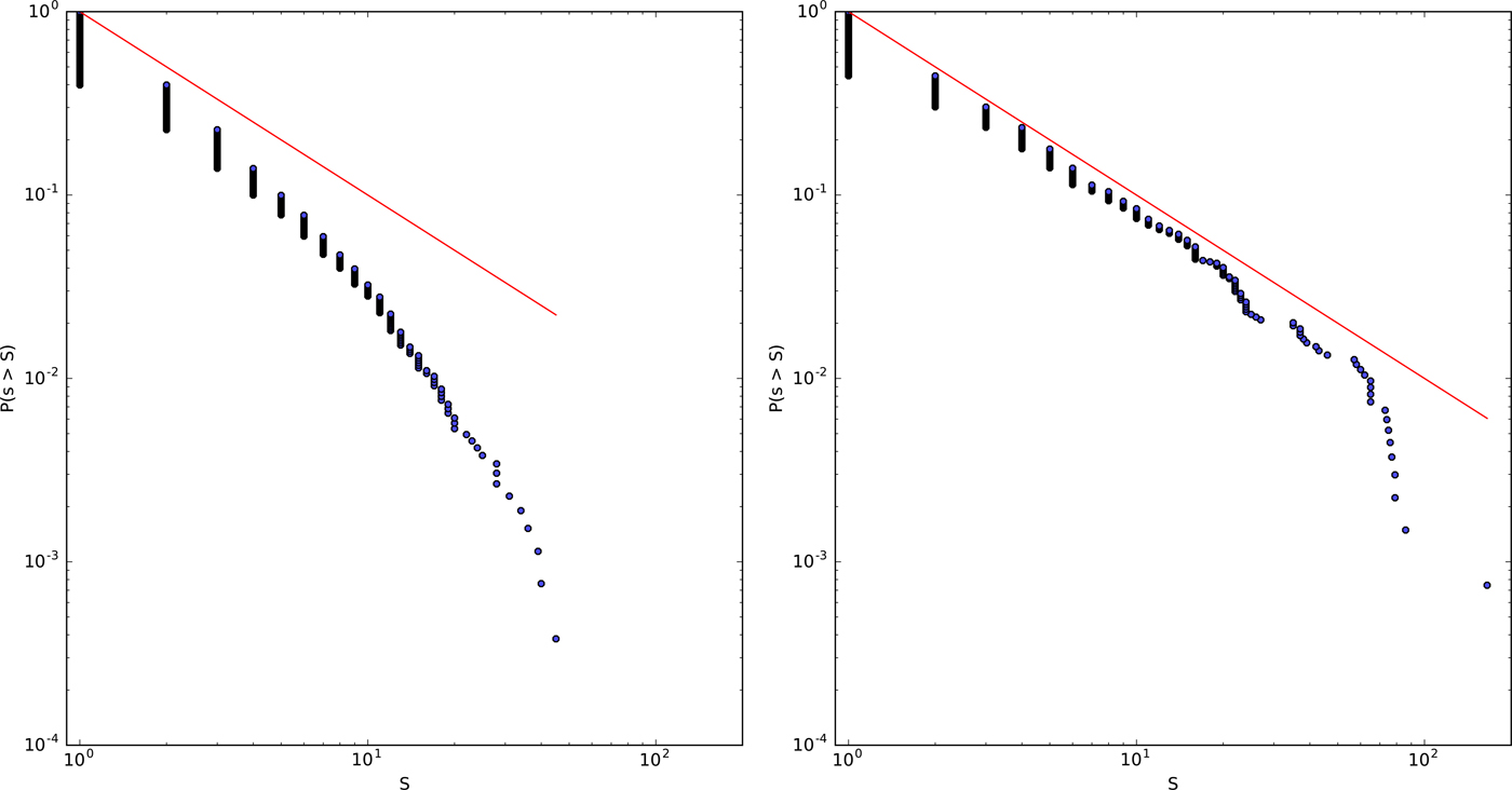
What is the distribution of voids sizes? In Fig. 3 we plot, for β = 15 and 25, the complementary cumulative distribution function (CCDF) P(s > S), which measures the probability to find a void with size s larger than S. We prefer to show the CCDF instead of the usual distribution P(s) because it is monotonic and more smooth. We see some scale invariance, P(s > S)∝S −a, with a≈1, which means that P(s)∝S −a–1. The cluster is a quasi-fractal and the cut-off for large S is mostly a finite size effect.
Complementary cumulative distribution P(s > S) of void sizes for β = 10 and 25. The straight line with exponent −1 is a guide for the eyes.
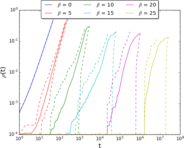
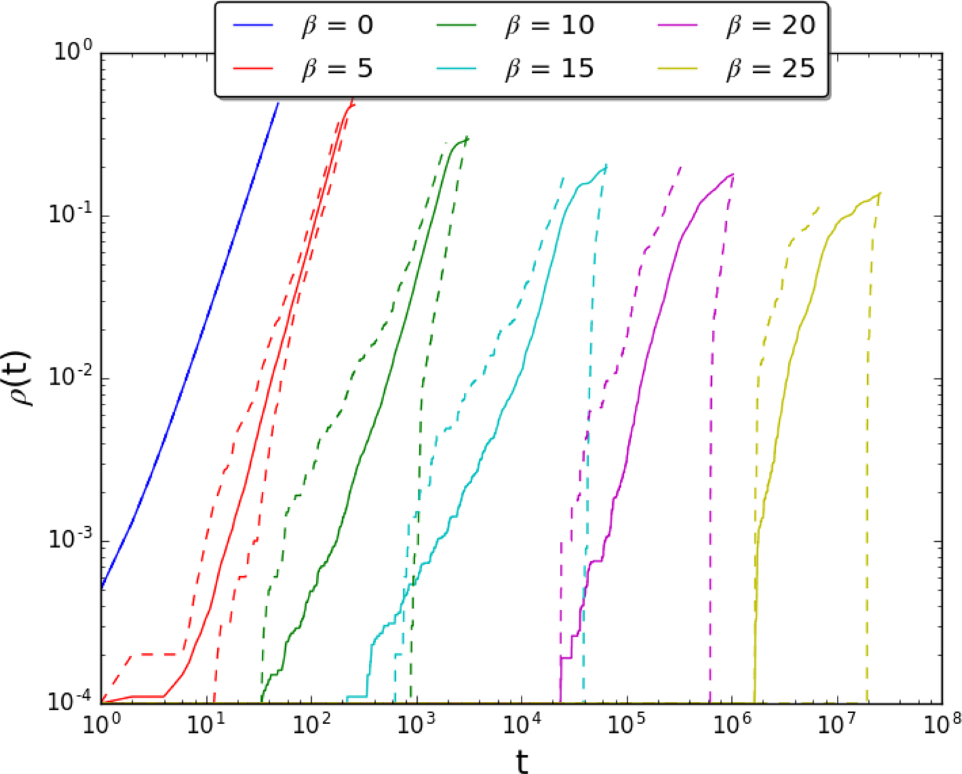
If n(t) is the number of colonized sites at time t, the density of colonized sites is ρ(t) = n(t)/L 2 = Σij Sij(t)/L 2. In Fig. 4, we show the density ρ(t) as a function of time. The colonization clusters grow as a delayed power law, which means that the GIP process is much slower than a normal diffusion for β > 5. We performed simulations over only ten runs because of the divergence of simulation times with β.
Density of visited sites ρ(t) for different values of β. Each solid curve is the average over ten runs. The dashed lines denote the maximum and the minimum ρ over these runs and gives an idea of the dispersion of the results.
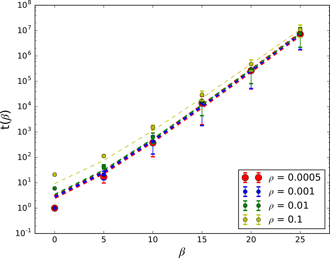
To better see this delayed colonization, we also show in Fig. 5 the mean colonization time t(β) (the time for the cluster, with a central seed, to achieve the density ρ of colonized sites). We found an approximate exponential dependence on β for β > 5, that is, t(β)∝exp(αβ). In our model, colonization times can vary by orders of magnitudes, indicating that the percolation time for the total GHZ can also vary by orders of magnitude. This delayed colonization time and the presence of large unvisited regions, are at the core of our proposed explanation for the Fermi Paradox.
Mean colonization time t(β) for different values of colonization density ρ as a function of diffusion difficulty β. We use a timescale where Δt = 1000 years and the vertical axis is given in years.
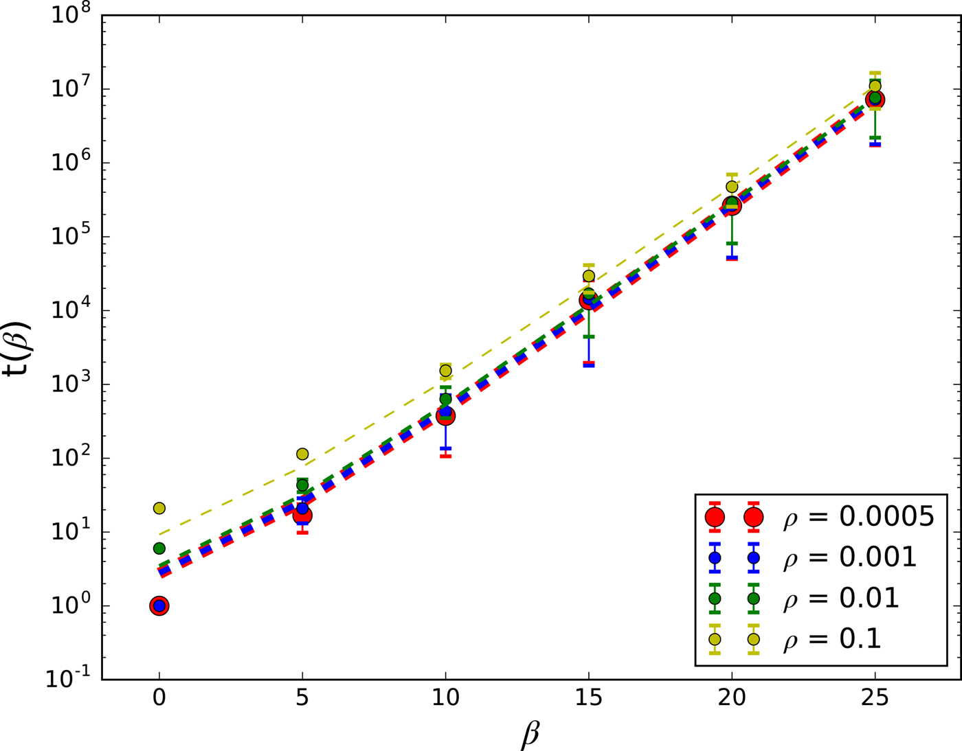
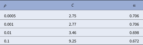
We can explain this exponential dependence on β. The expected colonization time for a single site is t 1 = 1/p(E) = exp(βE). To have a percolating cluster, we need that the final probability that a site is colonized is α≳p c = 0.592 (p c is the threshold value for site percolation in square lattices). For the uniform distribution P(E), this is equivalent to require that, in the final cluster, most sites have E < α. Integrating t 1 = exp(βE) with a normalized distribution valid for the colonized sites P(E) = 1/α Θ(α− E) leads to an expected colonization time per site of <t 1> = 1/(αβ) [exp(αβ)−1]. The total colonization time t(β) is a multiple of this time, so it is a lower bound. We have used the function y = C (αβ)−1 [exp(αβ)−1] to fit the curves. Our simple calculation predicts α≳0.592 and C > 1, which is compatible with the simulations, see Table 1.
Curve fit parameters: y = C (αβ)−1 [exp(αβ)−1]

The run times of the algorithm depend on the number of sites of the percolating cluster. The cluster seems to scale as N∝Ld with d < 2 (the ideal percolating cluster has fractal dimension d = 91/48≈1.896). So, run times scale basically as exp(αβ) Ld, which is a good scaling with L to implement larger simulations (the problem is the exponential prefactor). For β = 25, we have an I7 processor run time of about 20 h.
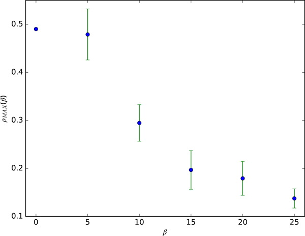
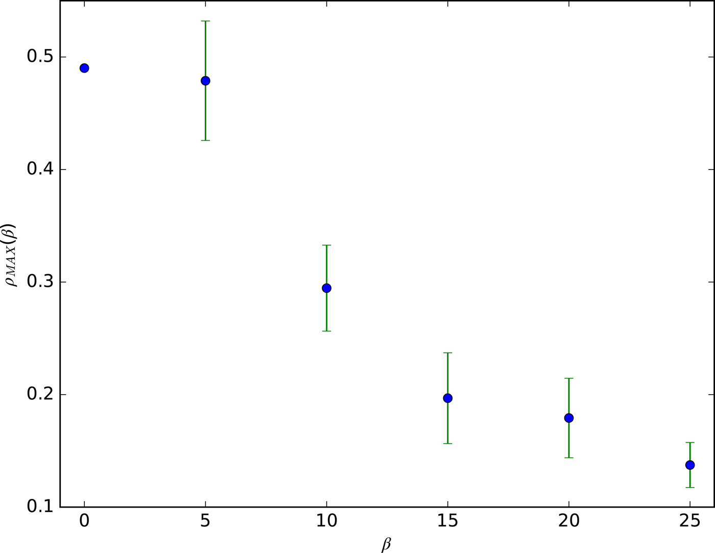
The final density of the clusters decreases with β, that is, the volume of the voids increase with β, as can be seen in Fig. 6. This occurs because all clusters with finite β are supercritical and a perfect fractal only occurs in the β→∞ limit.
Final density of the colonization clusters as a function of β. With higher β, we have less dense (with more voids) clusters.
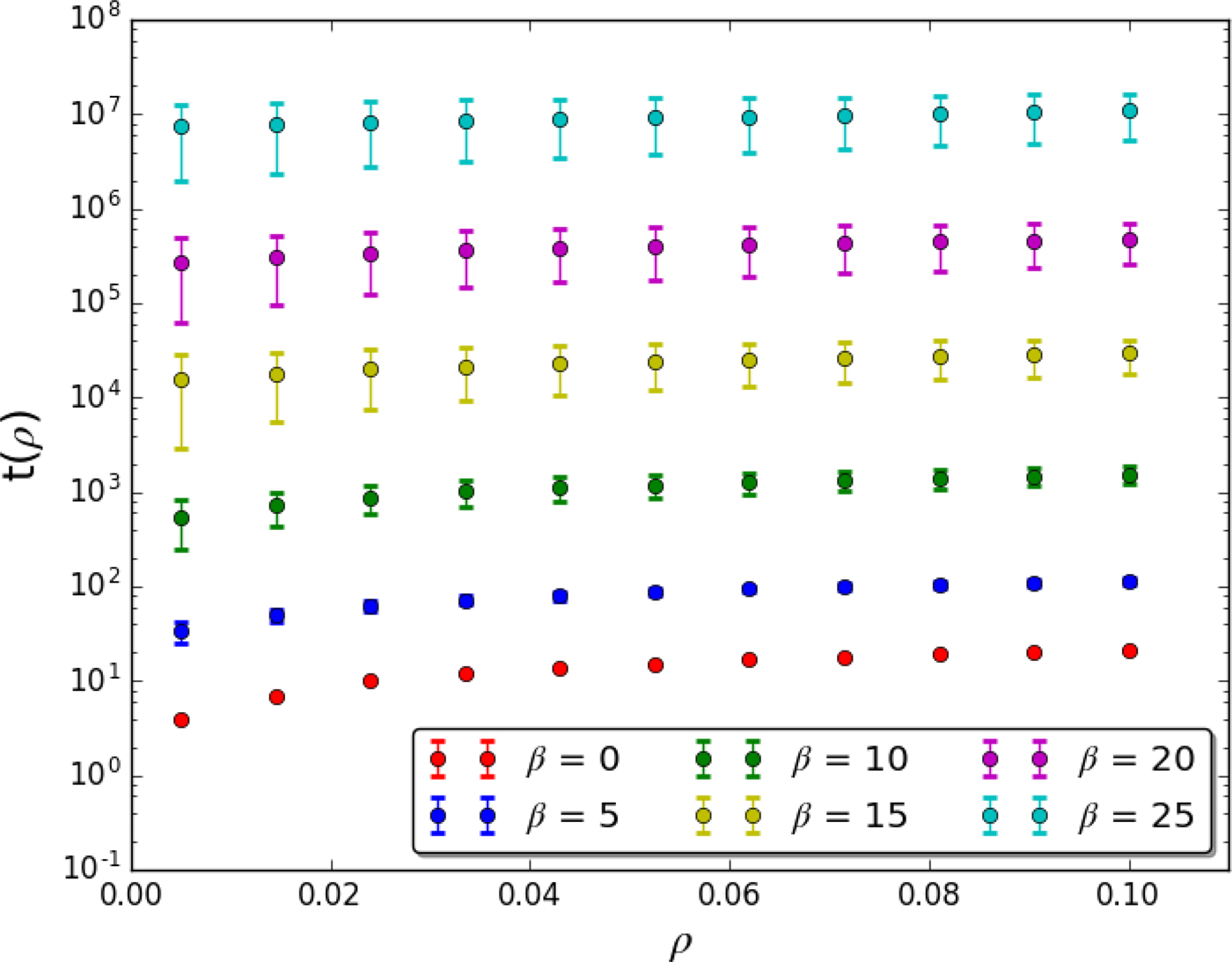
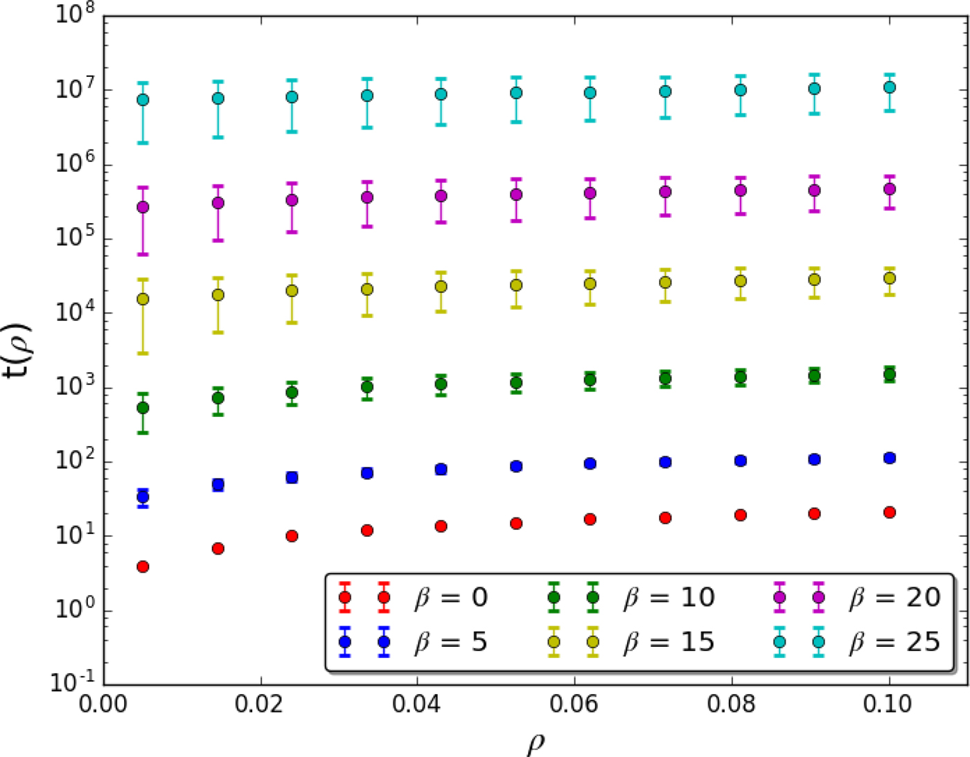
The dependence of colonization times on ρ is less relevant, not changing the order of magnitude of t(ρ), as can be seen in Fig. 7. Although our simulations are done in a square of area A = 1000 × 1000 ly2, it is clear that the same trends of Figs. 5 and 7 will be observed in a GHZ of area H × B ly2. In particular, we can do an order of magnitude extrapolation: for example, with β = 25, t(ρ)≈107 (Fig. 7), we can estimate a percolation time for the GHZ (with area ≈2800A) as at least 2800 × 107 = O(1010) years. This is of the order of the age of the Galaxy and well above the conventional estimates for galactic colonization (Hart Reference Hart1975).
Mean colonization time t(ρ) for different values of difficulty parameter β as a function of colonization density ρ. We use a timescale where Δt = 1000 years and the vertical axis is given in years.
Discussion
Recent progress in astrobiology suggests that life could be very probable in the Galaxy (Rossmo, Reference Rossmo2017). This means that discussions about SETI and Fermi Paradox turn out more relevant. The simplest solution is that some factors produce inevitably subcritical colonization clusters, including single sites clusters and even non-coexisting civilizations in time (Webb Reference Webb2015).
In contrast, IP and other fractal-like cluster growth models allow for supercritical colonization of the Galaxy where the cluster of colonized sites percolates through the GHZ. Our GIP model, with its vast empty regions and slowing down of the colonization timescales, solves Fermi Paradox without appealing to non-testable sociological assumptions about galactic civilizations such as the zoo hypothesis or singularity convergence (Webb Reference Webb2015). In this sense, our GIP colonization is a minimal model.
The main advantage of our GIP model, in contrast to the standard IP model, is that it enables the introduction of a physical timescale, see Fig. 5. Notice that our model produces always a supercritical cluster, but colonization times diverge exponentially with β. The model instantiates at the same time two explanations for the Fermi Paradox: colonization times could be very large (β large) and Earth could be inside a huge empty region, since the colonization cluster has (almost) scale-invariant voids.
Another advantage of our model is that it is a minimal model having only one free parameter (β). This enables the full study of the (rich) phenomenology of the model. In contrast, other colonization models of the literature, as Vukotic & Cirkovic (Reference Vukotic and Cirkovic2012), have a plethora of free parameters so that the study of possible model behaviours are very difficult.
The exponential dependence on β (including the large simulation times) is of course due to the choice of the exponential p(E). Other choices are possible. For example, Landis (Reference Landis1998) model is equivalent to use a step function p(E) = Θ(P−E) and produces a percolating cluster with large voids if we choose P≈p c. All sites that can be colonized are equal and the time to colonize a site is a single time step, <t 1> = t 1 = 1. The total colonization times (and computer run times) are very fast but no delayed colonization effect can be observed.
The time step Δt = 1000 years has been used also in the percolation model of Hair & Hedman (Reference Hair and Hedman2013). In contrast to Landis model, but like our model, there are repetitive attempts to colonize the same site with a constant probability p = C, where C is a characteristic of the mother sites (propensity to colonize, uniform and fixed from start). In this case, each open site has the same expected time to be colonized <t > = 1/C which is not very high.
Hair & Hedman (Reference Hair and Hedman2013) showed that, due to the repetitive attempts to colonization, there is no formation of large voids. They claim that their model does not support the percolation solution for Fermi Paradox. Apparently, these authors have not noticed that it is this particular choice p = C that is the cause of the elimination of the voids. Our model does not suffer from this shortcoming because the exponential colonization probability p(E) mimics the IP process of colonizing first the easier sites that produce fractals. Of course, since there is no strict prohibited sites, in contrast to Landis (Reference Landis1998) model, there occurs a very slow occupation of such voids, in another timescale, a kind of ageing effect. Figure 2 shows instantaneous photos at the exact time of percolation. With more time, our configuration of voids is not static (as in Landis (Reference Landis1998) model), which is also a realistic colonization feature. Of course, we can explore other scenarios by changing the colonization function p(E). An interesting (and faster) function could be a power law p(E) = 1/(1 + E)β.
Other advantage of the model is that, in contrast to Landis (Reference Landis1998) model where fractals appear only near E c≈p c and like IP (which is an example of self-organized criticality (SOC)), our GIP model fractality (criticality) is generic, in the sense that the large β limit is a gross tuning, not fine tuning. The exact percolation threshold p c is not a parameter of our model.
Concerning the distribution of colonization barriers, we have assumed P(E) uniform in the interval [0,1] as in the original IP model. However, in the colonization context, perhaps other distributions reflect better the colonization difficulty, for example, a log-normal distribution where easy to colonize sites are more rare. This is not a model limitation but a generalization: we can run the GIP with any P(E). The main influence of a different P(E) is not in the form of the cluster or the distribution of void sizes. After all, for the cluster to percolate, we need to colonize the neighbours with a probability at least of p c and this condition is independent of P(E). The main difference will be in colonization times: for example, with less easy sites as in the log-normal case, the colonization times would increase but the formation of large voids will continue.
We have not discussed multi-seed (multi-source) colonization. Our results for large β produce quasi-fractal clusters with very irregular borders and deep intrusions of uncolonized sites. Starting with different seeds leads to the formation of coexisting domains (supposing that invasion of an already colonized site is prohibited). For civilizations with different technology level T = 1/β, the faster growing civilization will colonize the open sites at these deep open spaces of the slow growing civilization.
In the model, it is possible to colonize only neighbours’ sites. Of course, we could relax this constraint, allowing long-range colonization. The random neighbour (mean-field) version of the model would correspond to science-fiction civilizations with warp drives of infinite range. In the mean field version, each colony tries to colonize some site at any distance. This model produces independent clusters and voids, not a single colonization cluster, even starting from a single seed. An intermediary case could be to allow colonization of sites at distance D < D max≠1.
A limitation of our model is that the parameter β does not evolve with time, that is, there is no important technological evolution T(t) = 1/β(t) of the CCs. Indeed, strong technological evolution means that β decreases with time, so that the fractal voids disappear in a faster way. However, any decreasing function for β(t) would be by now highly speculative. Therefore, an assumption of our model is that the technological evolution β(t) is never strong enough to turn out the colonization cluster in a compact Eden-like aggregate, that is, in our model the colonization difficulty never falls below β≈15.
Another limitation of the GIP is that colonies never die. This, however, is easily introduced in the model, say by giving a death probability d per unit of time to each colony, or even a non-uniform d(E ij), which increases with the habitability barrier. This shall not change our main results, since a death rate favours the creation of larger empty voids and delayed colonization.
Anyway, these can be viewed not as true limitations but as the advantage of concrete computational models (in contrast to only verbal explanations, as done in most the literature about Fermi Paradox (Webb Reference Webb2015)). With computational models, we can add new parameters and features, incrementally improving the potential explanations and the comparison with astrobiological data.
We notice that our GIP model is original and has not been studied in previous statistical physics literature. As a technical point, we observe that it does not produce a strict 2d percolation fractal (only the IP process produces that, with the same percolation density p c≈0.592 and fractal dimension d f = 91/48≈1.896 of standard static percolation (Wilkinson & Willemsen Reference Wilkinson and Willemsen1983; Sheppard et al. Reference Sheppard1999)). Our clusters for finite β are not exactly critical, but supercritical. The IP process is approximated in the limit β→∞. However, as we have already observed, this means a strong divergence in percolation time limβ→∞ t(β) = limβ→∞ C exp(αβ)→∞.
This is a signal of what is called an absolute separation of timescales in the SOC literature (Jensen Reference Jensen1998). Indeed, IP is considered the first example of an SOC system, proposed even before the sand pile model of Per Bak (Jensen Reference Jensen1998). The absolute separation of timescales (the computational time to detect what is the site with the lowest barrier E ij in the cluster contour cannot be compared with the site colonization time) is the main problem that prevents to apply standard IP to colonization problems and that is solved here by our GIP process with a well-defined timescale Δt.
We can infer the fact that we possibly inhabit a void from a weaker form of Fermi Paradox, that we call Proximal Fermi Paradox. If there are CCs close to the Earth, they already had time to reach us. Therefore, there are no CCs close to the Earth and we are inside a (perhaps large) colonization void.
Proximal Fermi Paradox means that there is a radius R from the Earth that does not have CCs. Either the galactic civilization branching process is subcritical, due to some reasons as discussed by Webb (Reference Webb2015), or we are inside a large void in a quasi-fractal supercritical colonization cluster. A general prediction is that the probability of SETI detection of CCs diminishes for exoplanets inside the radius R (of course, SETI detection of non-CCs is outside our argument). Although we have no data for estimating R, an order of magnitude guess could be R = O(103) ly. SETI null results (Harp et al. Reference Harp2016; Enriquez et al. Reference Enriquez2017) are fully compatible (indeed required) by the IP solution.
We can make a particular prediction if we accept the hypothesis that a full-developed biosphere, early or late, enables the emergence of CCs within a finite variance time (i.e. emergence times are not highly skewed). Suppose that CCs are (at least probable) attractors of some self-organization process in biospheres, especially for planets older than Earth. In other words, although the probability p of emergence of a CC is very low (if compared with the number N of non-technological species that form a biosphere), the huge number of species evolved makes the expected value for a CC to emerge in a biosphere as Np = O(1).
We are not affirming that this hypothesis – significantly old biospheres lead to CCs with probability O(1) – is true, we only use it here as an auxiliary lemma to derive another prediction. Thus, under this hypothesis, Proximal Fermi Paradox and the idea of colonization voids predict that search for bio signatures in potentially habitable exoplanets close to us in older stars as Proxima-b (Anglada-Escude et al. Reference Anglada-Escude2016), Tappist-1 (Gillon et al. Reference Gillon2017), Tau Ceti (Feng et al. Reference Feng2017) or Ross128 (Bonfils et al. Reference Bonfils, Astudillo-Defru, Diaz, Almenara, Forveille, Bouchy, Delfosse, Lovis, Mayor, Murgas, Pepe, Santos, Segransan, Udry and Wunsche2017, arXiv:1711.06177) shall give null results. That is, not only SETI search in old exoplanets close to us will fail, but also biosphere biomarker detection in old exoplanets will fail, under the auxiliary hypothesis that old biospheres must lead to CCs that should have colonized us a long time ago.
Finally, we observe that, although the Earthlights photo of Fig. 1 inspired our ideas, our GIP process does not intend to model the complex sociological–ecological–economic factors that drive true colonization on Earth. Our GIP is only a toy model that illustrates how huge empty voids and delayed expansion can arise even in very simple colonization processes. It shows the sufficient ingredients to produce the phenomena, not the realistic detailed ones. The same observation applies when comparing our GIP model with more detailed simulations of the galactic colonization (Vukotic & Cirkovic Reference Vukotic and Cirkovic2012).
Conclusion
For solving Fermi Paradox, we have basically two options: the galactic civilization cluster is inexistent or subcritical (several motives for this are discussed in Webb (Reference Webb2015)) or Fermi assumption about a normal diffusion colonization with compact clusters is erroneous. In this paper, we explored the consequences of this last possibility, firstly proposed by Landis (Reference Landis1998), where the colonization process creates supercritical clusters with large voids. Our model also shows that colonization times can vary by orders of magnitude depending on colonization difficulty, which aids to explain why the galactic civilization has not reached us yet.
We have also detected a shortcoming in Hair & Hedman's (Reference Hair and Hedman2013) model: its failure in producing large voids is due to the use of a homogeneous and constant colonization probability per time step. Our model, with its exponential colonization probability, produces large voids, instantiating the percolation solution for Fermi Paradox in a more realistic way than Landis (Reference Landis1998) does.
To explain the great silence, we need not assume any sociological factor and purposeful action of a galactic UN. It suffices that we lie in a very probable but apparently exotic place. Therefore, we must consider whether humans are typical or exotic like the lost Amazonian tribe or, perhaps better, inhabitants of an oasis surrounded by a huge desert. That is, what is the probability P(E∈V) that Earth is inside a large empty region (a void V)? To evaluate this, we notice that, like in observer-dependent anthropic reasoning, the information that we are here (as an independent biosphere I) is important: the relevant quantity is the conditional probability P(E∈V | I), which is much larger than P(E∈V), since independence I requires that we inhabit a region with no CCs close to us. If we have neighbouring CCs, they would have colonized Earth a long time ago.
If the percolation solution to Fermi Paradox is correct, then Earth location is atypical, belonging to a huge but poorly inhabited galactic domain. We must consider the distressing possibility that we live not in the highly developed part of the Galaxy, similar to the regions full of light points in the Earth photo, but in a large region analogous to Amazon, Sahara or Siberia. Earth might not be a typical but an exotic place, being an isolated site far away from the galactic civilization.
We must all perform a change of viewpoint about what is typical and what is exotic (this fact motivated our early joke about exotic Americans and typical Brazilians). The opposite view that we are the unique or the first technological civilization of the Galaxy (Crawford Reference Crawford2000; Ward & Brownlee Reference Ward and Brownlee2004; Webb Reference Webb2015) or the Star Trek expectation that one day we will be the ‘leaders’ of the United Federation of Planets probably originates from a misplaced developed world perspective. Perhaps, it is simply wishful thinking: we ‘wish’ that this could be true because we cannot accept that we pertain to an isolated, underdeveloped, forgotten region in galactic terms. As a literary antidote to these naive views, we recommend the books of Stanislaw Lem (Lem Reference Lem1988; Lem Reference Lem1999).
Acknowledgements
The authors thank George C. Cardoso for discussions and an anonymous referee for several important suggestions including the elaboration of Fig. 3. EG thanks a CAPES fellowship and GRG thanks financial support from USP. OK acknowledges the support from CNAIPS-USP. This paper was produced as part of the activities of FAPESP Research, Innovation and Dissemination Center for Neuromathematics (grant #2013/07699-0, São Paulo Research Foundation).