I. INTRODUCTION
X-ray microscopy has grown to be a field with innumerable applications in biology, archaeology, medicine, materials research, and others, and an adequate review covering all these fields could fill many books. In this article, we give an overview of recent progress and impending challenges of correlative X-ray microscopy in the field of photovoltaics, limiting ourselves to studies that include:
-
(i) Correlative microscopy, i.e. mapping of multiple parameters with sub-micrometer resolution.
-
(ii) Application to photovoltaic material or device investigation.
-
(iii) Utilization of X-rays generated by synchrotrons, as they are the only X-ray source that can provide brilliant beams for microscopy (to our knowledge, correlative microscopic photovoltaic research utilizing X-ray free electron lasers or laboratory X-ray sources has not yet been reported).
There is a good reason for this limitation: unlike other fields of microscopy, the investigation of photovoltaic materials and devices demands new concepts of correlative microscopy, like simultaneously measuring different parameters such as electrical performance and elemental distribution. Therefore, this branch of X-ray microscopy is confronted early on with new challenges that inherently come with the development of new techniques, and the achievements directly relate to other fields where correlative approaches are being developed for in situ and operando experiments.
A. Outline
We will briefly discuss opportunities and challenges in solar cell research (Sec. I.B), with the unique capabilities of hard X-ray microscopy to study nanoscale inhomogeneities and defects. We will discuss in greater detail the technique of X-ray beam induced current (XBIC) in Sec. II, as tremendous progress has been made in the understanding of XBIC measurements in the last few years. The historic development of XBIC is presented in Sec. II.A. Highlighting the difference between XBIC and a more broadly known technique, total electron yield (TEY), in Sec. II.B, we elucidate different aspects of XBIC measurements. These are specified in further subsections of Sec. II and may range anywhere from sample preparation (Sec. II.C) and fundamentals about electrical connections for these operando measurements (Sec. II.D) to the further analysis that enables the conversion of XBIC signal to charge collection efficiency (Sec. II.E).
In Sec. III, we discuss the challenge of a paradigm change: while early research on silicon devices approximated solar cells as X-ray transparent matrices for XBIC and X-ray fluorescence (XRF) microscopy, this approximation is no longer justified for thin-film solar cells. After the description of the challenge in Sec. III.A, we demonstrate a first solution in Sec. III.B. This approach, however, is too simplistic for future applications, giving rise to the need for more sophisticated correction approaches to be implemented into the analysis of more complex device architectures. An outlook to future correction approaches is given in Sec. III.C.
Finally, we showcase examples of correlative X-ray microscopy applied to solar cells over the last 5 years utilizing state-of-the-art techniques and equipment at several synchrotron beamlines. Section IV.A gives an example how XRF measurements (in this case, impurity measurements in silicon) can serve as experimental fundament for widely applied numerical models (here, a diffusion model to simulate different steps during solar cell fabrication). In Sec. IV.B, the effect of grain boundaries and elemental distribution on charge collection efficiency is discussed, based on simultaneous XBIC and XRF measurements of CuInxGa1−xSe2 (CIGS) solar cells. Section IV.C showcases an example of in situ measurements, where XRF measurements enabled the tracking of elemental segregation, melting, and crystallite formation during growth of a CIGS solar cell absorber layer.
In Sec. IV.D, we discuss applications of correlative X-ray microscopy to solar cells with organic absorber layers: due to the low atomic number of the elements of interest, scanning transmission X-ray microscopy (STXM) and scattering is utilized with polarized soft X-rays, which enables the extraction of domain clusters with similar orientation.
Section IV.E focusses on the characterization of nanowires by hard X-rays. Combining high-resolution XRF, X-ray diffraction (XRD) and X-ray absorption near edge spectroscopy (XANES) with X-ray excited optical luminescence (XEOL) allows for the correlation of composition and structure with optical properties, and for direct testing of quantum confinement.
In Sec. IV.F, we demonstrate how X-ray microscopy can unveil compositional variations even in complex structures such as perovskite solar cells, and how image processing has enabled analysis beyond the qualitative comparison of images. Finally, Sec. IV.G describes correlative XBIC and XRF measurements applied to perovskite solar cells deposited on a mesoporous scaffold, which does not allow for the same type of analysis.
Beyond the application to thin-film solar cells, we are certain that these types of experiments significantly contribute to the understanding of functional materials and complex devices. It is crucial that such investigations are conducted not only at the appropriate scale, where the relevant chemical, physical, and electrical processes take place, but also under conditions that represent varying operating environments. Therefore, Sec. V gives an outlook on correlative X-ray microscopy of the coming one or two decades, and we give additional insight into the possibilities and challenges that arise with newly available synchrotron beamlines and measurement techniques.
B. The need of X-ray microscopy for solar cells research
There is no doubt that photovoltaics (PV) will play a major role in electricity supply during the next decades. In the past years, dramatic cost reductions in mass manufacturing have led to an increase in installed PV power, surpassing even optimistic forecasts: more than 200 GWp was installed by the end of 2015, with an impressive average compound annual growth rate of 45% observed since 1975. Reference Louwen, van Sark, Faaij and Schropp1 Today, grid parity has been reached in many of the large economies worldwide and solar energy contributes significantly to electricity generation. Reference Breyer and Gerlach2,Reference Masson and Brunisholz3
This increase in solar deployment will come with new challenges on different levels: the abundance of materials can become an issue Reference Green4,Reference Jean, Brown, Jaffe, Buonassisi and Bulovic5 ; efficiency and lifetime of modules need to be improved for lower levelized cost of electricity (LCOE) and a smaller ecological footprint; materials need to be recycled, and less energy-intensive processes and materials need to be found to reduce the energy-payback time.
These challenges demand a high level of continuous research in the field of PV, and although many of the effects are visible at the module level, their causes lie at the nanoscale, which elicits the need to investigate the materials at that scale. Moreover, cell efficiencies get closer to their theoretical limits and complex device architectures are being sought. Therefore, the engineering approach for the design and optimization of solar cells calls for advanced characterization methods. Reference Shockley and Queisser6–Reference Sheng, Bower, Bonafede, Wilson, Fisher, Meitl, Yuen, Wang, Shen, Banks, Corcoran, Nuzzo, Burroughs and Rogers9
This is the case throughout the entire lifecycle of the solar cell, from the distribution of elements and defects during solar cell growth as well as the charge-collection and recombination during operation, to degradation and failure mechanisms due to impurity diffusion, crack formation, and irradiation- and heat-induced cell damage.
The behavior of solar cells is very often limited by inhomogeneously distributed nanoscale defects. Reference Bertoni, Fenning, Rinio, Rose, Holt, Maser and Buonassisi10,Reference Buonassisi, Istratov, Marcus, Lai, Cai, Heald and Weber11 This has been known for a while in the field of crystalline silicon, Reference Morishige, Jensen, Hofstetter, Yen, Wang, Lai, Fenning and Buonassisi12–Reference Bernardini, Johnston, West, Lai, Naerland, Stuckelberger and Bertoni18 but the truth is that they are far more abundant in polycrystalline materials, and are the limiting factor in thin-film solar cells where grain sizes are often on the order of the diffusion length. Reference Siebentritt19–Reference de Quilettes, Vorpahl, Stranks, Nagaoka, Eperon, Ziffer, Snaith and Ginger24
Furthermore, inhomogeneities in the elemental distribution of multi-component thin-film semiconductors such as CdTe, CIGS, and perovskites can play an important role. Reference Luo, Gamliel, Nijem, Aharon, Holt, Stripe, Rose, Bertoni, Etgar and Fenning25 For decades, polycrystalline absorbers like CdTe and CIGS with adjacent junction and contact layers have been optimized following a trial-and-error approach, and the development of different layers for perovskite solar cells has followed similar trends. At the initial stages of a technology development this approach is powerful. It has led to remarkable solar cell efficiencies of 22.6% (CIGS), 22.1% (CdTe), and 22.1% (perovskite); Reference Green, Emery, Hishikawa, Warta, Dunlop, Levi and Ho-Baillie26 all of which now outperform multicrystalline silicon (mc-Si) solar cells with a maximum efficiency of 21.3%. Reference Green, Emery, Hishikawa, Warta, Dunlop, Levi and Ho-Baillie26 The next step in device optimization requires fine tuning and significant improvement of the fundamental understanding of limiting defects. Given that optimization steps at higher levels are generally less efficient in terms of R&D$/W, these processes could directly benefit from in situ and operando approaches, by which functional materials with defects can be understood rather than optimized by empiricism, and designed rather than found by chance.
Hard X-rays have unique capabilities well suited to probe complex materials and devices. They have excellent penetration of capping layers and interfaces, enabling 3D imaging of full devices and buried structures. They can penetrate gases and fluids, enabling studies at pressure, and under process conditions. They allow quantitative studies of sample composition with trace-element sensitivity in structured materials and devices. Chemical-state information of individual atomic species can be obtained using X-ray spectroscopic techniques. X-rays do not interact with external fields, and thereby enable studies in electric or magnetic fields. With the development of optics capable of focusing hard X-rays to ever smaller dimensions, hard X-ray beams with sizes of 50 nm and well below now allow probing nanoscale regions of materials and devices. As such, they are capable of studying the compositional and structural properties of defects, inhomogeneities and gradients in devices and functional materials, under a large variety of synthesis and operating conditions.
Soft X-rays do not offer the high penetration of hard X-rays and related advantages for in situ measurements and probing of encapsulated solar cells. However, they are more sensitive to light elements that are particularly important for organic solar cells or as trace elements/impurities in solar cells with inorganic absorber layers. This leads to similar experimental difficulties for soft X-ray- Reference Crumlin, Liu, Bluhm, Yang, Guo and Hussain27 as for electron-beam Reference Abou-Ras28 based techniques, where the surface sensitivity demands extensive sample preparation and adapted equipment for in situ and operando measurements of solar cells, which sets application limits. The high penetration of hard X-rays combined with high sensitivity of elemental distribution, structure, and spatial resolution is a key argument for correlative microscopy based on hard X-rays: no other technique—neither electron-beam based techniques nor nano-scale secondary ion mass spectroscopy (SIMS) Reference Senoner and Unger29 —offer non-destructive in situ and operando evaluation of solar cells in similarly broad applications.
How will nanoscale X-ray characterization in photovoltaics look like in 10 years? With a resolution below the 10 nm scale, methods that leverage functionality, systematic and correlative imaging, and above all statistical meaningfulness in multiple dimensions will drive the research field. Reference Merkle, Lechner, Steinbach, Gelb, Kienle, Phaneuf and Chawla30–Reference Sakdinawat and Attwood32 The impact of the dramatic increase in dimensionality—enabled by high-brilliance beamlines, progress in detector technologies, measurement and analysis techniques—cannot be overestimated for correlative X-ray microscopy.
II. X-RAY BEAM INDUCED CURRENT—A POWERFUL MEASUREMENT TECHNIQUE TO MEASURE ELECTRICAL PERFORMANCE AT THE NANOSCALE
As the technique of XBIC measurements for the evaluation of the electrical performance of solar cells or other electronic devices is known only to a highly specific community, we introduce in this section the fundamentals of this powerful technique. In particular, the electrical connection scheme of proper XBIC measurements is worth a short discussion, as experimental artifacts of XBIC measurements can be suppressed or enhanced by the choice of the measured charge carrier and of the grounding.
A. The short history of XBIC measurements
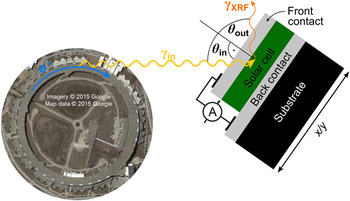
Strictly speaking, X-ray beam induced current techniques have been used for many decades, be it in the form of ionization chambers, drift detectors, or even scintillators that are read out through photomultiplier tubes. In all these cases, the measured current is at first approximation proportional to the number of absorbed X-ray photons. Instead, we consider X-ray beam induced current in a narrower sense, where the device of interest serves as the detector itself, in which a current is generated by X-ray excited electron–hole pairs. For the separation of electron–hole pairs in the device of interest, different approaches are utilized: whereas solar cells rely on charge separation by the electric field spanned by an internal p–n junction or on charge-carrier selective contacts, other devices such as ion chambers rely on an externally applied electric field. Using secondary beam-intensity detectors—such as up-stream ion chambers—the XBIC signal from our device under investigation can be normalized to the beam intensity, and microscopic scanning of the device across a focused X-ray beam enables the assessment of either areas of varying X-ray absorption, or of varying charge recombination efficiency which is highly valuable for electronic devices such as solar cells.
Enabled by the development of highly focused synchrotron beamlines for X-ray microscopy, and motivated by the growing interest in recombination and charge collection efficiency in solar cells, Hieslmair, et al. proposed and demonstrated the first XBIC measurements investigating crystalline silicon solar cells in the year 2000. Reference Hieslmair, Istratov, Sachdeva and Weber33 For over ten years, XBIC was applied by only few research groups and uniquely to silicon solar cells. Reference Buonassisi, Heuer, Vyvenko, Istratov, Weber, Cai, Lai, Ciszek and Schindler15–Reference Vyvenko, Buonassisi, Istratov and Weber17,Reference Vyvenko, Buonassisi, Istratov, Hieslmair, Thompson, Schindler and Weber34–Reference Vyvenko, Buonassisi, Istratov, Weber, Kittler and Seifert47 Although most XBIC applications utilized a synchrotron as the X-ray source and combined the electrical with X-ray fluorescence measurements as demonstrated in Fig. 1, laboratory-source applications were demonstrated too Reference Fahrtdinov, Feklisova, Grigoriev, Irzhak, Roshchupkin and Yakimov48–Reference Shabelnikova and Yakimov54 with a sensitivity to recombination that can be higher than using electron-beam induced current (EBIC) measurements. Reference Shabel’nikova and Yakimov55,Reference Shabel’nikova, Yakimov, Grigor’ev, Fahrtdinov, Bushuev and Bushuev56 The disregard of thin-film solar cells had not only opportunistic but also technical reasons. On one hand, only the development of a hard X-ray nanoprobe beamline, Reference Winarski, Holt, Rose, Fuesz, Carbaugh, Benson, Shu, Kline, Brian Stephenson, McNulty and Maser57 created in 2012, would have high enough spatial resolution for thin-film solar cells with sub-micrometer-sized absorber-layer crystallites. On the other hand, difficulties with signal interpretation from optically dense thin-film absorbers negated the excellent sensitivity of X-ray fluorescence for the mapping of metal impurities in the X-ray transparent silicon matrix (see Sec. III for a more thorough discussion). Only in the last few years, the focus of XBIC measurements has shifted from silicon to thin-film solar cells including CIGS, Reference West, Husein, Stuckelberger, Lai, Maser, Stripe, Rose, Guthrey, Al-jassim and Bertoni58–Reference Stuckelberger, West, Husein, Guthrey, Maser, Al-Jassim, Stripe, Rose and Bertoni62 CdTe, Reference Stuckelberger, West, Husein, Guthrey, Maser, Al-Jassim, Stripe, Rose and Bertoni62 organic, Reference Watts, Queen, Kilcoyne, Tyliszczak, Hellman and Ade63 and perovskite Reference Stuckelberger, Nietzold, Hall, West, Werner, Ballif, Rose, Fenning and Bertoni64,Reference Stuckelberger, Nietzold, Hall, West, Werner, Niesen, Ballif, Rose, Fenning and Bertoni65 absorber layers.
Simultaneous measurement of X-ray fluorescence photons (γXRF) and of the X-ray beam induced current (A) at a synchrotron beamline. The measurement geometry represents the constraints given at the nanoprobe beamline 26-ID-C Reference Winarski, Holt, Rose, Fuesz, Carbaugh, Benson, Shu, Kline, Brian Stephenson, McNulty and Maser57 at the Advanced Photon Source at the Argonne National Laboratory, where the sum of the angle between the incident beam and the excident fluorescence photons is fixed to 90° by the vacuum-chamber geometry. For highest resolution (at the cost of enhanced self-absorption of the fluorescence photons), typical values for the angles are θin = 15°, θout = 75°.

Significant milestones in the development of XBIC measurements and correlative X-ray microscopy of solar cells are highlighted in Fig. 2. The improvement in measurement sensitivity and the decrease in spotsize enabled first grain boundary measurements of multicrystalline silicon and later of CIGS and perovskite solar cells. In parallel, progress was made in the statistical analysis and correlation of simultaneously measured parameters. The high sensitivity of XRF set the experimental fundament for diffusion models of impurities in silicon (impurity-to-efficiency simulator I2E), Reference Hofstetter, Fenning, Bertoni, Lelievre, Del Canizo and Buonassisi66 and the quantitative correlation between elemental distribution and charge collection efficiency in CIGS solar cells served as direct feedback to solar cell growers for the engineering of high-efficiency devices. There is no end in sight for further developments in correlative X-ray microscopy of solar cells. To name a few, correction algorithms, time-resolved in situ measurements, and feature recognition algorithms for particle tracking and statistical analysis are hot topics under development that will partially be discussed later in this article.
Milestones of the application of X-ray microscopy to solar cells: report of the first XBIC measurement of multi-crystalline silicon (mc-Si) by Hieslmair et al., Reference Hieslmair, Istratov, Sachdeva and Weber33 of the first XBIC/XRF correlation applied to CIGS solar cells by West, et al., Reference West, Husein, Stuckelberger, Lai, Maser, Stripe, Rose, Guthrey, Al-jassim and Bertoni58 and of the first XBIC/XRF measurements of perovskite solar cells by Stuckelberger, et al. Reference Stuckelberger, Nietzold, Hall, West, Werner, Ballif, Rose, Fenning and Bertoni64 These developments were paralleled by statistical analyses such as the dependence of distribution and size of iron precipitates in silicon on solar cell processing steps by Fenning, et al., Reference Fenning, Hofstetter, Bertoni, Hudelson, Rinio, Lelievre, Lai, Del Canizo and Buonassisi103 or the pixel-by-pixel correlation between charge collection efficiency and elemental composition in CIGS solar cells by West, et al. Reference West, Husein, Stuckelberger, Lai, Maser, Stripe, Rose, Guthrey, Al-jassim and Bertoni58 Top left figure reprinted from “New synchrotron-radiation based technique to study localized defects in silicon: “EBIC” with X-ray excitation” by H. Hieslmair, A.A. Istratov, R. Sachdeva, and E.R. Weber. In the National Renewable Energy Laboratory report “10th Workshop on Crystalline Silicon Solar Cell Materials and Processes: Extended Abstracts and Papers. Workshop held 14–16 August 2000, Copper Mountain, Colorado” (August 2000), http://www.nrel.gov/docs/fy00osti/28844.pdf. Accessed January 18, 2017. Top center and bottom right figure © 2015 IEEE. Reprinted, with permission, from B. West, S. Husein, M. Stuckelberger, B. Lai, J. Maser, B. Stripe, V. Rose, H. Guthrey, M. Al-Jassim, and M. Bertoni, “Correlation between grain composition and charge carrier collection in Cu(In,Ga)Se2 solar cells”, IEEE PVSC proc. (2015). Top right figure © 2016 IEEE. Reprinted, with permission, from M. Stuckelberger, T. Nietzold, G.N. Hall, B. West, J. Werner, C. Ballif, V. Rose, D.P. Fenning, and M.I. Bertoni: Elemental distribution and charge collection at the nanoscale on perovskite solar cells. IEEE PVSC proc. (2016). Bottom left figure reprinted from, D.P. Fenning, J. Hofstetter, M.I. Bertoni, S. Hudelson, M. Rinio, J. F. Lelievre, B. Lai, C. Del Canizo, and T. Buonassisi: Iron distribution in silicon after solar cell processing: Synchrotron analysis and predictive modeling. Appl. Phys. Lett. 98, 16 (2011), with the permission of AIP Publishing.

B. Total electron yield versus XBIC
Measurements of photoelectrons are widely utilized, and we distinguish between two cases that are fundamentally different from a measurement point of view, although both measure in the widest sense a current induced by X-rays. In both cases, the measurement is based on the excitation of an electron by incoming X-rays resulting in its ejection from the material into vacuum in the first case (if the electron does not have enough energy to leave the sample, e.g., because it was excited well below the sample surface, it recombines without any measured signal), or in its excitation at least across the band gap in the second case.
In the first case, an electron detector directly counts free electrons that are emitted from the surface. This approach is most widely used in X-ray photoemission electron microscopy (XPEEM), or energy-filtered XPEEM/X-ray photoelectron spectroscopy (XPS), for which the free electrons are not only counted but their kinetic energy is also evaluated. As the electron detector does not cover the full solid angle, into which electrons are ejected, the electron detector current is a poor measure of the total electron yield. This measurement technique is not related to XBIC; in fact, emitted photoelectrons can be measured simultaneously as XBIC.
In the second case, photoelectrons are measured indirectly: being absorbed, e.g., at the grounded chamber walls, the electrons need to be replaced at the sample surface to maintain charge neutrality in the sample. Therefore, the replacement current is a measure of the ejected electron current, and normalized to the incident photon flux, it is a measure of the total electron yield (TEY). The left current circuit in Fig. 3 shows exemplarily the setup of a TEY measurement applied to a perovskite solar cell; due to the high surface sensitivity, only the TEY of the topmost layer, in this case indium tin oxide, is probed.
Setup of a perovskite solar cell for total electron yield (TEY, left current circuit, with electrons collected at the chamber wall CW) and X-ray beam induced current (XBIC, right current circuit) as shown in Ref. Reference Stuckelberger, Nietzold, Hall, West, Werner, Niesen, Ballif, Rose, Fenning and Bertoni65. Blue dots represent end-of-trajectories of secondary electrons, generated in the absorber layers by 9 keV X-ray photons incident through the back contact into the solar cells. The abbreviations in the layer stack indicate: ITO—indium tin oxide; IOH—hydrogen-doped indium oxide; spiro-MeOTAD—N 2,N 2,N 2′,N 2′,N 7,N 7,N 7′,N 7′-octakis(4-methoxyphenyl)-9,9′-spirobi[9H-fluorene]-2,2′,7,7′-tetramine; MAPI—methylammonium lead iodide.

The right current circuit in Fig. 3 shows the setup for XBIC measurements. Instead of ejected surface electrons as in TEY measurements, XBIC measures the electron–hole pairs that are generated by incident X-ray photons in the absorber layer, substantially in the same manner, as during standard solar cell operation, during which photons in the visible or near-infrared spectral range excite electrons from the valence band to the conduction band in the semiconducting absorber layer. Generated electrons in the conduction band and holes in the valence band diffuse or drift to the n- and p-type doped semiconductors on either side of the device, where they are collected. Closing the external circuit and measuring the current therein—most often, under short-circuit conditions—yields the XBIC signal.
Related to the high energy of the primary X-ray photons, there are significant differences between standard solar cell operation or laser-beam induced current (LBIC), and XBIC measurements. Whereas low-energy photons can excite a maximum of one electron across the band gap, Footnote a and the excess energy is lost through thermalization of the hot carriers, this is not true for high-energy photons: through photon–electron and electron–electron interactions, a cascade of secondary particles is generated that leads to multiple excitations of electrons from the valence to the conduction band. As the secondary particle interactions typically take place at a different location than the interaction of the primary X-ray photon with matter—in particular, secondary fluorescence photons can travel long distances before they are re-absorbed—the electron–hole pair generation is spatially distinct from the path of the incident X-ray beam. For the illustration of this effect, we have used PyPenelope Reference Pinard, Demers, Salvat and Gauvin67 that is based on the software package Penelope Reference Salvat, Fernandez-Varea, Acosta and Sempau68 for a 3D Monte-Carlo simulation of the particle–matter interaction in the perovskite solar cell stack that is shown in Fig. 3. As a result, blue dots in the absorber layer represent the end-of-trajectories of slowed-down electrons. At these spots, the electrons thermalize and enter the band structure. From here on, the physics of charge collection and recombination is the same as for the electron excitation by low-energy photons, only the yield and distribution is different. Further details about the simulation and actual XBIC measurements that we have performed on such solar cells are reported in Ref. Reference Stuckelberger, Nietzold, Hall, West, Werner, Niesen, Ballif, Rose, Fenning and Bertoni65. Whereas the yield for X-ray-to-electron conversion is discussed in Sec. II.D, we are working on a publication focusing on the spatial distribution of generated electron–hole pairs that define the interaction volume, for XBIC measurements in comparison with EBIC measurements. Reference Stuckelberger, West and Bertoni69
Note that both generated charge carriers, electrons and holes, always need to be collected, otherwise they recombine. Therefore, only electron–hole pairs generated in the absorber layer can contribute to the XBIC signal, whereas electrons and holes generated in the hole- and electron-transport layers (HTL and ETL) or adjacent transparent-conductive oxides (TCOs) or other layers recombine as one of the charge carriers cannot cross the p–n junction. Footnote b For this reason, the end-of-trajectory distribution of electrons is not shown for any other layer except for the absorber layers.
Simultaneous measurements of TEY and XBIC are fundamentally excluded. In most cases—in particular for hard X-rays—the XBIC signal is orders of magnitude larger than the TEY signal, such that the TEY signal would maximum contribute to a small error of XBIC measurements. However, there are exceptions, where poor experiment design or conductance can lead to misinterpretation of TEY as XBIC. These include: (a) For very low X-ray energies and/or strongly absorbing layers upstream of the solar cell absorber layer, only a small amount of X-ray photons may reach the absorber layer. (b) If the solar cell is shunted or poorly connected, electron–hole pairs generated in the absorber layer may recombine without being measured in the external circuit. (c) For cross-section measurements of thin solar cell lamellae or otherwise thin absorber layers (in extreme case 2D materials), the absorptance is too small to generate a large XBIC signal.
C. From sample preparation to XBIC measurements
In principle, in situ and operando measurements of solar cells should require the least amount of sample preparation, as they shall be studied by definition in their environment and during operation. In practice, however, highly sophisticated experimental setups are required, as synchrotrons cannot be brought to the native environment of solar cells, and it therefore is necessary to reproduce such environments around the solar cell for testing and to simulate operating conditions. Nevertheless, the approach of minimal sample preparation remains: the goal is to measure working devices, and often the only sample preparation needed is cutting the solar cell to fit the beamline geometry and electrically contacting them. This is in strong contrast to other techniques providing nanometer-scale resolution such as scanning (SEM) or transmission electron microscopy (TEM): due to the small penetration depth of electrons, thin lamellae need to be lifted out (often not allowing for operando measurements) otherwise the information depth of measurements is limited to the very top of a solar cell. For the same reason, the creation of the appropriate environment is far more challenging for probing with electrons than for probing with hard X-ray photons that travel with ease through millimeters of a gas under ambient pressure. Further details about the penetration depths of electrons and X-ray photons in different semiconductors and solar cell stacks is given in Refs. Reference Stuckelberger, West, Husein, Guthrey, Maser, Al-Jassim, Stripe, Rose and Bertoni62, Reference Stuckelberger, Nietzold, Hall, West, Werner, Ballif, Rose, Fenning and Bertoni64, and Reference Stuckelberger, Nietzold, Hall, West, Werner, Niesen, Ballif, Rose, Fenning and Bertoni65, and a publication dedicated to this subject is in preparation. Reference Stuckelberger, West and Bertoni69 For a comparison of the penetration depth of X-rays in silicon and common thin-film absorber layers, we refer to Sec. III.A and Fig. 8.
Whereas the high penetration depth of hard X-ray photons is often an advantage, there are drawbacks: the interpretation of plan-view images of overlaying structures of the same material, like multiple layers of grains, becomes challenging. The combined signal from them can often not be deconvoluted, and solar cells with single-grain absorber thickness are required to resolve the performance of single grains or grain boundaries (this is not the case if other effects shall be investigated such as grain-independent electrical performance, shunts, or substrate effects). Similarly, probing samples with hard X-rays in cross section is more challenging but possible as showcased in Ref. Reference Stuckelberger, West, Husein, Guthrey, Maser, Al-Jassim, Stripe, Rose and Bertoni62.
Contacting the p and n side of solar cells is critical, and creative solutions often need to be found for the adaptation of XBIC measurements to a beamline. For low shunting probability without sacrificing signal/noise ratio or adding series resistance, we use typically thin Au or Cu wires between the solar cell and a support that carries the solar cell and is mounted on the scanning stage. Depending on the solar cell surface, we use silver paint, graphite paint, conductive tape, or mechanical pressure for electrical contact between the wire and the solar cell. At the solar cell support structure, we change from the thin wires to lower-resistance cables, ideally shielded coaxial cables, that are connected to the chamber feed through or directly to the current amplifier (most often, we use the Stanford Research Systems Preamplifier SR570). For measurements at sub-100-nm resolution, it is crucial that the electrical connections do not transfer vibrations onto the sample. For measurements at the scale of hundreds of nanometers, this is less critical. For the combination of operando with in situ XBIC measurements at high spatial resolution, we have modified the low-vibration heating stage described in Ref. Reference Chakraborty, Serdy, West, Stuckelberger, Lai, Maser, Bertoni, Culpepper and Buonassisi70 for XBIC compatibility.
From the point of view of high-speed data collection in correlative microscopy mode, a practical issue is always the correct synchronization of data acquisition from the measurement of different parameters during operando measurements. Ideally, the same unit processes the acquisition of multiple measurements such as XBIC and XRF. For example, the voltage output from current preamplifiers can serve as input to voltage/frequency converters, which enables the recording of XBIC exactly as an ionization chamber (if there is no free channel available, down-stream detector channels can often be used, as no signal is recorded for the case of full, thick solar cell devices that are intransparent for X-rays).
D. How to ground properly for XBIC measurements?
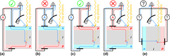
In contrast to EBIC measurements, where grounding is intuitively important to avoid charging of the sample by the incoming electron beam, grounding for XBIC measurements has hardly been discussed in literature. For most X-ray microscopy measurements such as XRF, charging of a sample is not critical. However, it needs to be avoided for electrical measurements. As detailed in Sec. II.B, highly energetic electrons can leave the sample surface, constituting the TEY current but contributing to error for XBIC measurements. In the vast majority of XBIC probed devices, more electrons leave the sample at the side that is exposed to the incoming X-ray photons, Footnote c hence, the front side Footnote d of the device should be grounded as highlighted in Fig. 4. Note that it is irrelevant for this choice whether the front side is n type or p-type: in the former case, electrons constitute the replacement current from the front contact to the spot of missing electrons, in the latter, holes constitute the replacement current from the spot of missing electrons to the front contact. In either way, no replacement current flows across the p–n junction of the probed device to make it to the back contact where it can contribute to the XBIC signal.
Different grounding schemes for X-ray beam induced current (XBIC) measurements. Due to the replacement current of ejected surface electrons that are collected at the chamber wall (CW) and shall be measured to evaluate the total electron yield (TEY) but can contribute to the error in XBIC measurements (subpanels b and d), the side exposed to the incoming X-ray beam should be grounded, be it the n side (subpanel a) or the p side (subpanel c). In the case of cross-section measurements (subpanel e), the situation is less clear and we lack of specific experimental data. However, it is probably wise to ground the side that is of the type of the majority carrier in the absorber layer.

Except for Ref. Reference Stuckelberger, West, Husein, Guthrey, Maser, Al-Jassim, Stripe, Rose and Bertoni62, we are not aware of reports of cross-section XBIC measurements. Obviously, the cross-section surface that is exposed to the incident X-ray photons must not be grounded as a contact there would short-circuit the p–n junction. For this case, we suggest to consider grounding the side that is of the type of the majority carrier in the absorber layer (p for CIGS, CdTe, and perovskite, n or p for Si), as the replacement current will be constituted of these carriers.
E. Converting XBIC signal into charge collection efficiency
After the back-conversion from the recorded signal to actual X-ray beam induced current, the question remains how the qualitative variations in current maps can be converted into a quantitative charge collection efficiency (CE) that we define as the ratio of collected
 $\hbox( {N_{{{\rm{e}}^ - }{\rm{/}}{{\rm{h}}^ + }}^{{\rm{coll}}}} \hbox)$
to generated
 $\hbox( {N_{{{\rm{e}}^ - }{\rm{/}}{{\rm{h}}^ + }}^{{\rm{gen}}}} \hbox)$
electron–hole pairs:
 $${\rm{CE:}} = {{N_{{{\rm{e}}^ - }{\rm{/}}{{\rm{h}}^ + }}^{{\rm{coll}}}} \over {N_{{{\rm{e}}^ - }{\rm{/}}{{\rm{h}}^ + }}^{{\rm{gen}}}}}\quad .$$
The charge collection efficiency is of fundamental interest in every solar cell and quantifies the probability of converting photons into current, and recombination losses (1 − CE) which should be minimized.
How can the CE be measured? In the photovoltaics community, the external (EQE) and internal quantum efficiency (IQE) are widely known as
 $${\rm{EQE:}} = {{N_{{{\rm{e}}^ - }{\rm{/}}{{\rm{h}}^ + }}^{{\rm{coll}}}} \over {N_{{\rm{ph}}}^{{\rm{in}}}}}{\rm{and\ IQE:}} = {{N_{{{\rm{e}}^ - }{\rm{/}}{{\rm{h}}^ + }}^{{\rm{coll}}}} \over {N_{{\rm{ph}}}^{{\rm{abs}}}}}\quad .$$
Here,
 $N_{{\rm{ph}}}^{{\rm{in}}}$
denotes the number of incident photons, and
 $N_{{\rm{ph}}}^{{\rm{abs}}}$
the number of absorbed photons. For incident photons in the visible range (VIS) of the solar spectrum (relevant for typical photovoltaics applications), the generation of more than one electron–hole pair per incident photon is negligible. This allows for the approximation
 $$N_{{{\rm{e}}^ - }{\rm{/}}{{\rm{h}}^ + }}^{{\rm{gen}}}\mathop \approx \limits^{{\rm{VIS}}} N_{{\rm{ph}}}^{{\rm{abs}}}\quad .$$
Most solar cell measurements use a back reflector such that the transmittance T is negligible, and the absorptance A = 1 − T − R reduces to
 $$A\mathop \approx \limits^{{\rm{VIS}}} 1 - R\quad ,$$
where R denotes the reflectance. Approximations (3) and (4) justify
 $${\rm{CE}}\mathop \approx \limits^{(3)} {{N_{{{\rm{e}}^ - }{\rm{/}}{{\rm{h}}^ + }}^{{\rm{coll}}}} \over {N_{{\rm{ph}}}^{{\rm{abs}}}}} = {\rm{IQE}}\mathop \approx \limits^{(4)} {{N_{{{\rm{e}}^ - }{\rm{/}}{{\rm{h}}^ + }}^{{\rm{coll}}}} \over {N_{{\rm{ph}}}^{{\rm{in}}} \cdot (1 - R)}} = {{{\rm{EQE}}} \over {1 - R}}\quad .$$
Therefore, IQE and EQE are often interpreted as charge collection efficiency. Both are measurable using standard laboratory equipment with an absolute error in the order of 1%, originating predominately from the reference cell calibration. Reference Emery71 The relative error between measurements using the same setup can be well below the reference-cell error.
Even without taking into account corrections of CE that will be discussed in the next section, we seek to extract a parameter such as IQE or EQE from XBIC measurements. However, approximations (3) and (4) cannot hold for XBIC measurements, because high-energy X-ray photons generate an entire electron shower, and a high fraction of photons can be transmitted through the solar cell.
Footnote e
The level of complexity of this analysis increases given that: first, parasitic X-ray absorption in layers other than the absorber layer can exceed absorption in the absorber layer by orders of magnitude whereas parasitic absorption in the VIS is small and quantifiable by laboratory measurements. Second, down-conversion of photons, which has a limited impact on
 $N_{{{\rm{e}}^ - }{\rm{/}}{{\rm{h}}^ + }}^{{\rm{gen}}}$
in the VIS, has a major impact on
 $N_{{{\rm{e}}^ - }{\rm{/}}{{\rm{h}}^ + }}^{{\rm{gen}}}$
for X-ray photons through fluorescence.
Therefore, Eq. (3) for X-ray photons needs to include a correction factor C:
 $${\rm{XCE:}} = {{N_{{{\rm{e}}^ - }{\rm{/}}{{\rm{h}}^ + }}^{{\rm{coll}}}} \over {N_{{{\rm{e}}^ - }{\rm{/}}{{\rm{h}}^ + }}^{{\rm{gen}}}}}\mathop = \limits^{{\rm{X - ray}}} {{N_{{{\rm{e}}^ - }{\rm{/}}{{\rm{h}}^ + }}^{{\rm{coll}}}} \over {C \cdot N_{{\rm{ph}}}^{{\rm{in}}}}}\quad .$$
Strictly speaking, the X-ray charge collection efficiency XCE is identical to CE but the “X” indicates that the assumptions typically made for VIS photons are not valid for X-ray photons. While
 $N_{{{\rm{e}}^ - }{\rm{/}}{{\rm{h}}^ + }}^{{\rm{coll}}}$
and
 $N_{{\rm{ph}}}^{{\rm{in}}}$
are measureable as the X-ray beam induced current and the incident photon flux, respectively, we need to introduce a factor C for the ratio of generated electron–hole pairs per incident X-ray photon. Several factors contribute to C, and we could approximate it through C ≈ A·B, where A is the absorptance of the absorber layer (the fraction of absorbed photons), and B is the number of generated electron–hole pairs per absorbed X-ray photon. For purely qualitative analysis, Eq. (6) suggests that the XBIC signal—normalized to
 $N_{{\rm{ph}}}^{{\rm{in}}}$
—may be interpreted as XCE as long as C can be assumed constant. This is generally the case for solar cells with low variations in layer thicknesses (including all layers from window layers to the substrate). Apart from metallization areas, wafer-based silicon solar cells typically meet this criterion, but not thin-film solar cells such as cells with CdTe or CIGS absorber layers. Here, C depends strongly on the absorber layer thickness, and secondary particle interactions need to be considered. Neglecting such secondary particle interactions, the utilization of C ≈ A·B is minimally successful as a quantitative analysis of XCE. Instead, we suggest calculating C as
 $$C \approx {{{E_{{\rm{abs}}}}} \over {\alpha \cdot {E_{{\rm{ph}}}}}}\quad ,$$
where E abs is the energy deposited in the absorber layer per incident photon with the energy E ph, and α accounts for the energy efficiency of electron–hole pair generation. Whereas E ph is usually well known for a given experiment, the determination of E abs and α require a more in-depth discussion.
One may think that E abs could easily be calculated through Beer–Lambert’s law. However, this neglects secondary particle generation, by assuming all of the energy is deposited at the spot where the attenuation takes place. As a matter of fact, photoelectric absorption of X-rays by core electrons is dominant for hard X-ray absorption (see e.g., Fig. 4 in Ref. Reference Stuckelberger, Nietzold, Hall, West, Werner, Niesen, Ballif, Rose, Fenning and Bertoni65). Consequently, X-ray fluorescence photons can carry a significant amount of energy out of the layer of interest—or into them from adjacent layers.
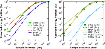
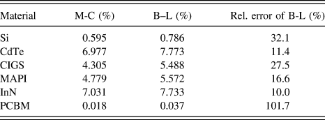
A quantitative evaluation of the deposited energy for different absorber materials and absorber thickness is given in Fig. 5, using Beer–Lambert’s law (no secondary particle interaction) and Monte–Carlo methods (including secondary particle interactions). Footnote f Note that for thin absorber layers, Beer–Lambert’s law overestimates the deposited energy by more than an order of magnitude, whereas it asymptotically converges toward the values obtained by Monte-Carlo simulation for thicker absorber layers. For numerical comparison at absorber layer thicknesses of 1 μm, Table I summarizes the differences between the two models.
Fraction of absorbed energy in solar cell absorber layers as a function of the absorber thickness, for incident X-ray photons with an energy of 10 keV and different absorber materials: CdTe, InN, Si, CuIn0.3Ga0.7Se2 (CIGS), CH3NH3PbI3 (MAPI), and Phenyl-C61-butyric acid methyl ester (PCBM). We have calculated the absorbed energy fraction using Monte-Carlo (M-C) methods (Penelope software package Reference Salvat, Fernandez-Varea, Acosta and Sempau68 ) and using Beer–Lambert’s law. Note that the absorption coefficients of CdTe and InN, and of CIGS and MAPI are very close such that the absorbed-energy-fraction curves overlap.

Fraction of absorbed energy in solar cell absorber layers, for incident X-ray photons with an energy of 10 keV and different absorber materials of 1 µm thickness: Si, CdTe, CuIn0.3Ga0.7Se2 (CIGS), CH3NH3PbI3 (MAPI), InN and phenyl-C61-butyric acid methyl ester (PCBM). We have calculated the absorbed energy fraction using Monte-Carlo (M-C) methods (Penelope software package Reference Salvat, Fernandez-Varea, Acosta and Sempau68 ) and using Beer–Lambert’s law (B-L).

Due to the complex nature of secondary-particle effects such as exiting fluorescence photons, photoelectrons, or multiple scattering that depend strongly on the material stack and photon energy, there is no general rule for when Monte–Carlo simulations are necessary, and when Beer–Lambert’s law suffices. As an example of this complexity, we have simulated the energy deposited in a 2-µm-thick CuIn0.3Ga0.7Se2 absorber layer from 10 keV incident photons using Penelope. For the case of a free-standing layer, E abs = 891 eV of the incident energy E ph = 10,000 eV are deposited in the absorber layer. If the same absorber layer is simulated on top of 100-nm-thick Mo, 70-nm-thick Ti, and 50-µm-thick stainless steel—reproducing the layer stack of flexible CIGS solar cells as reported in Ref. Reference Pianezzi, Chirilă, Plösch, Seyrling, Buecheler, Kranz, Fella and Tiwari72—E abs = 1015 eV are deposited in the CIGS layer. The additional energy comes from fluorescence photons (here predominantly FeK photons) from the substrate that are emitted toward the CIGS layer. For Beer–Lambert’s law, E abs is obviously the same for the free-standing layer and the layer on top of the substrate.
Although we like to emphasize the power of Monte–Carlo simulations for the most accurate, quantified, evaluation of the charge collection efficiency, Beer–Lambert’s law is of more practical use to calculate E abs. The main reason is that Monte–Carlo simulations would need to be re-run for each layer stack, i.e., for each pixel of an XBIC map with varying layer thicknesses. In contrast, the layer thicknesses that can be obtained pixel-by-pixel from simultaneous XRF measurements, can serve as input to calculate E abs analytically through Beer–Lambert’s law. This approach is further justified by the consideration of different error contributions of XCE. Although detectors for X-ray beam intensity measurements (normally P–I–N photodiodes made of Si) can be calibrated with an error between 0.4 and 2.3% Reference Gottwald, Kroth, Krumrey, Richter, Scholze and Ulm73 similar to reference cells for VIS, calibrated X-ray detectors are not as readily available. Furthermore, the energy-dependence of the detector responsivity as well as errors in the signal amplification add complexity. The lack of calibrated X-ray detectors permanently installed at synchrotron beamlines is a strong barrier for absolute XCE measurements. However, the largest error arises in most cases from the uncertainty in the layer thickness: the device structure of thin-film solar cells is often poorly known (layer composition, density), and layer thicknesses are often determined on sister samples of the probed solar cells with significant absolute errors. Inhomogeneities, lack of reproducibility, and measurement uncertainty contribute often to errors well above 10%, which translates into error for absolute XCE evaluation. At least with current methodology and experimental accuracy, errors of the absolute XCE as low as errors of equivalent CE for low-energy photons, are out of reach. The strength of XCE lies in relative comparisons of different regions within the same sample at high spatial resolution. In this case, error of the beam-intensity uncertainty, of α, and to some extent of layer thickness and density, cancel out, which leads to a greatly reduced relative error. The necessary correction of XCE for local thickness variations is discussed in Sec. III.B.
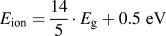
How can the parameter α be determined? As a matter of fact, absorbed energy translates at the end of particle showers mostly to free electrons that enter the band structure of the absorber material when their energy is on the order of the ionization energy E ion of a material. These hot electrons thermalize, and the energy between E ion and the band gap energy E g is mostly lost to heat without further conversion into electron–hole pairs. This justifies
 $$\alpha \approx {{{E_{{\rm{ion}}}}} \over {{E_{\rm{g}}}}}\quad .$$
Figure 6 shows a compilation of reported values of E
ion and E
g for a variety of solar cell absorber layers. Across different material systems, a linear relation between E
ion and E
g can be observed: whereas α ≈ 3 holds as a rule-of-thumb for absorbers such as Si or CdTe, a linear fit of all materials included in Fig. 6 yields E
ion = 1.875·E
g + 1.956 eV, and C.A. Klein suggested
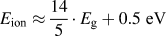 ${E_{{\rm{ion}}}} \approx {{14} \over 5} \cdot {E_{\rm{g}}} + 0.5\;{\rm{eV}}$
.
Reference Klein74
Note that for a given absorber material, α is only relevant for absolute XCE evaluation. For relative XCE measurements, α is only relevant in the case of spatially inhomogeneous absorber materials such as CIGS, where variations of the Ga/In ratio lead to variations of E
g and α; for uniform materials, α can be considered constant.
Ionization energy E
ion compared to the band gap E
g for a variety of semiconductors. The values are from Ref. Reference Alig, Bloom and Struck152 (Ge, Si, GaAs, CdTe, GaP, CdS, PbO, SiC), Ref. Reference Walsh and Butler153 (Cu2O, In2O3, ZnO), Ref. Reference Kasap and Rowlands154 (PbI2, GaSe, ZnTe, CdSe), Ref. Reference Emara, Schnier, Pourdavoud, Riedl, Meerholz and Olthof155 (MAPI), Ref. Reference Grant, Cunningham, Blue, O’Shea, Vaitkus, Baubas and Rahman156 (ionization energy of h-GaN), Ref. Reference Owens and Peacock157 (ionization energy of InP), Ref. Reference Awadalla158 (ionization energy of GaAsP), Ref. Reference Berger159 (band gap of InP, GaN), and Ref. Reference Pearton, Abernathy, Overberg, Thaler, Norton, Theodoropoulou, Hebard, Park, Ren, Kim and Boatner160 (band gap of GaAsP). The dashed blue line follows
 ${E_{{\rm{ion}}}} = {{14} \over 5} \cdot {E_{\rm{g}}} + 0.5\;{\rm{eV}}$
as suggested in Ref. Reference Klein74. The solid red line follows E
ion = 3·E
g. The dashed/dotted black line is a linear fit, following E
ion = 1.875·E
g + 1.956 eV.

III. A NEW CHALLENGE: FROM MEASUREMENTS OF TRANSPARENT MATRICES TO BULK MATERIAL
The lack of spatial resolution of hard X-ray microscopy beamlines for grain boundary analysis of thin-film solar cells was only part of the reason for the long-time focus of XBIC and XRF correlation to qualitative analysis of multicrystalline silicon solar cells. In this section, we investigate the problematics of correlative X-ray microscopy for thin-film solar cells and demonstrate how XBIC and XRF measurements can be performed and quantified.
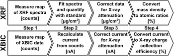
Figure 7 shows the typical workflow we perform at Arizona State University to analyze XRF and XBIC data taken from beamlines 2-ID-D, Reference Yun, Lai, Cai, Maser, Legnini, Gluskin, Chen, Krasnoperova, Vladimirsky, Cerrina, Di Fabrizio and Gentili75 21-ID-D, Reference Chen, Deng, Yuan, Flachenecker, Mak, Hornberger, Jin, Shu, Lai, Maser, Roehrig, Paunesku, Gleber, Vine, Finney, Vonosinski, Bolbat, Spink, Chen, Steele, Trapp, Irwin, Feser, Snyder, Brister, Jacobsen, Woloschak and Vogt76 or 26-ID-C Reference Winarski, Holt, Rose, Fuesz, Carbaugh, Benson, Shu, Kline, Brian Stephenson, McNulty and Maser57 at the Advanced Photon Source (APS) at the Argonne National Laboratory (ANL). While other workflows are possible and different methods may be used, these are established procedures used to analyze data published in Refs. Reference West, Husein, Stuckelberger, Lai, Maser, Stripe, Rose, Guthrey, Al-jassim and Bertoni58–Reference Stuckelberger, West, Husein, Guthrey, Maser, Al-Jassim, Stripe, Rose and Bertoni62, Reference Stuckelberger, Nietzold, Hall, West, Werner, Ballif, Rose, Fenning and Bertoni64, Reference Stuckelberger, Nietzold, Hall, West, Werner, Niesen, Ballif, Rose, Fenning and Bertoni65, Reference Chakraborty, Serdy, West, Stuckelberger, Lai, Maser, Bertoni, Culpepper and Buonassisi70, Reference West, Stuckelberger, Chen, Lovelett, Lai, Maser and Bertoni77, and Reference West, Guthrey, Chen, Jeffries, Bernardini, Lai, Maser, Shafarman, Al-Jasim and Bertoni78.
Flowchart for the analysis of X-ray fluorescence (XRF) and X-ray beam induced current (XBIC) measurements following a typical workflow for data acquired at the Advanced Photon Source and analyzed by the authors.

At APS, the MAPS software package Reference Vogt79 is used for XRF data acquisition (step 1). This includes the XRF measurement of a “standard”, taken with the same measurement geometry and during the same run. Such standards can be purchased from NIST 80 or AXO Dresden GmbH 81 with tabulated concentrations of a variety of elements. Standards can also be produced specifically for a given experiment if the conventional standards do not sufficiently cover the elements of interest. The thin-film approximation should be valid for the standard, such that self-absorption can be neglected.
Consequently, the raw counts of the XRF spectra—attributed to individual elements just by a simple detector-specific energy-binning—are fitted with MAPS. Footnote g This process isolates elements according to their fluorescence energies, quantifies their amount, and separates the fluorescence signal from background as well as from elastic/inelastic scattering contributions. A detailed description of the XRF data analysis using MAPS is in preparation. Reference Nietzold, West, Stuckelberger, Lai, Vogt and Bertoni82 For the quantification of the individual elements, the fitted integrated spectra are compared to the fitted spectrum of the standard reference, which yields the elemental distribution in µg/cm2 or nmol/cm2: being measured under the same conditions, effects of the fluorescence yield, geometry, detector sensitivity, etc. cancel out.
In the thin-film limit, where attenuation of the incident and excident X-ray beams can be neglected, the quantification from step 2 is final. Otherwise, the quantified elemental distributions need to be corrected for the attenuation—details of this correction are discussed in the following subsections. Note that the thin-film limit may apply for films that are as thick as 200 μm-thick Si wafers, if the incident energy and the fluorescence energy of the elements of interest are well above the absorption edge of the bulk material. In contrast, the thin-film limit does not apply for 2-μm-thick CIGS layers where the elements of interest constitute the bulk material as we discuss in section III.A.
As a fourth step, the corrected, quantified elemental distributions are normally converted to atomic ratios. Although this step is optional, it can be crucial for the interpretation: after step 3, the quantified elemental distribution is an area-density, and variations within maps are often governed by the topology of specific layers. For example, thin-film deposition yields often grains that are thicker than grain boundaries. For the analysis of stoichiometric comparisons, calculation of topology-independent atomic ratios is therefore more conclusive.
The XBIC signal is recorded like the signal from an ionization chamber as described in Sec. II.C together with the XRF data. As the measured current is typically very small (pA to µA range), noise and unwanted bias can lead to negative currents. This introduces the risk of inaccurate measurements, as the negative currents are converted into negative voltages (by the current amplifier) and chopped off by the voltage-to-frequency converter. To circumvent this problem, an offset voltage can be applied at the current amplifier, or both negative and positive currents can be measured by utilizing two voltage-to-frequency converters, and setting one of them with inverted polarity. In analogy to standard measurements for XRF measurements, the offset of XBIC measurements should be measured using the same conditions (including wiring) as for XBIC measurements but without incident X-ray photons.
The offset counts (generated by bias light, induced by external fields, or noise in the signal amplification) is subtracted from the measured XBIC signal. Afterward, the current is calculated from the known amplification steps. For typical measurement settings, the current preamplifier is set to 100 nA/V and the voltage-to-frequency converter to 105 cts/V which yields a factor of 10−3 nA/cts. Multiplied by the number of counts, this results in the current induced by the X-rays. Note that depending on the settings, dwell times different from 1 s may lead to an additional correction factor.
Similar as for XRF data, the XBIC signal highly depends on the topology. Therefore, a similar correction accounting for varying absorptance is applied to the XBIC signal, and the current is converted to the X-ray charge collection efficiency (see Sec. II.E for details).
A. The challenge
Why is it far more challenging to characterize thin-film solar cells by X-ray microscopy than wafer-based crystalline silicon? There are several aspects related to this question, and most of them can be reduced to the energy-dependence of the X-ray absorption coefficient.
Figure 8 shows the absorption or attenuation length—the depth, within which the X-ray beam intensity is reduced by a factor e. The left figure shows the attenuation length for bulk silicon (density 2.3 g/cm3) where the thin-film approximation holds in many cases. The right figure shows the attenuation length for bulk perovskite (methylammonium lead iodide (MAPI, CH3NH3PbI3) with density 4.0 g/cm3), representative for other thin-film solar cell absorber layers such as CdTe or CIGS, where the attenuation of the incident and excident X-ray needs to be taken into account.
Absorption length of Si (left, with density 2.3 g/cm3) and of CH3NH3PbI3 (right, with density 4.0 g/cm3). These graphs were generated from the energy-dependent mass absorption coefficient that was calculated using the functions “material.f” and “tables.f”, both being part of the Monte-Carlo simulation software package Penelope. Reference Salvat, Fernandez-Varea, Acosta and Sempau68

A complication is added by the fact that every type of thin-film solar cells contains elements of main interest with such high atomic numbers (Pb, I for MAPI, In for CIGS, Cd, Te for CdTe) that their quantification in nanoprobe hard X-ray beamlines requires the measurement of L or even M lines, for which reference data are less accurate than for K lines, branching ratios need to be considered, and their multiple occurrence tightens the problematics of signal separation from overlapping XRF peaks.
Last but not least, the elements of main interest in silicon solar cells are metal impurities such as Fe, Ni, or Cu with higher Z than Si. The absorption cross section of these elements is significantly larger than that of silicon, and the absorption length of Si at the corresponding K-fluorescence energies is large (compare e.g., the absorption length at 10 keV: 126.7 µm in Si, 17.4 µm in MAPI, 17.7 µm in CuIn0.3Ga0.7Se2 with 5.7 g/cm3, 12.4 µm in CdTe with 5.9 g/cm3). Footnote h In contrast, the elements of interest in thin-film solar cells are the main constituents themselves; the sensitivity to other elements with significant influence on device performance such as Na and K for CIGS is low, or even out of reach for hard X-rays in the case of elements such as nitrogen or oxygen.
The combination of these factors condensates to the statement that Si can be considered an essentially hard X-ray-transparent matrix with strongly absorbing heavy elements in low concentration, whereas thin-film solar cell absorber layers should rather be considered as bulk material for hard X-ray microscopy.
B. A first correction approach
Motivated by the above-mentioned need to consider thin-film solar cells as bulk material, we summarize here a simple correction that was suggested in Ref. Reference West, Stuckelberger, Jeffries, Gangam, Lai, Stripe, Maser, Rose, Vogt and Bertoni60 for the correction of XRF and XBIC data of CIGS solar cells.
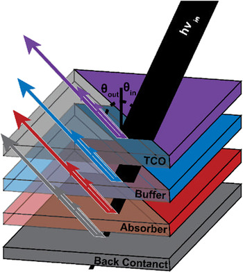
Figure 9 shows an example of a solar cell layer stack. The multiple arrows of varied length and thickness in each layer indicate different attenuation of the incident and excident X-ray photons for different elements in multicomponent layer stacks. The need of correction for attenuation becomes more important when measuring layers whose elements have large differences in atomic number, such as CIGS, Cu2ZnSnS4, or perovskites. This poses challenges not only in quantifying XRF spectra but XBIC data as well, because elements with larger attenuation coefficients will absorb more of the incident photons, leading to increased current.
Attenuation of an incident X-ray beam through multiple layers of a solar cell as shown in Ref. Reference West, Stuckelberger, Jeffries, Gangam, Lai, Stripe, Maser, Rose, Vogt and Bertoni60, with the top layer representing a transparent conducting oxide (TCO). Fluorescence photons generated in each layer are attenuated similarly as incident photons by the absorbing layer and the layers above it. Each element in a multicomponent layer has a unique energy-dependent attenuation coefficient causing fluorescence photons to be attenuated differently.

The main equation for the numeric correction of XRF data for a given solar cell architecture with T discrete layers Footnote i is
 $${I \over {{I_0}}} = {1 \over T}\sum\limits_{N = 1}^T {\exp \left[ {\sum\limits_{i = 1}^N {{{ - {\mu _{{\rm{in}}}}\left( {{t_i}} \right)} \over {\cos {\theta _{{\rm{in}}}}}}\Delta {t_i} + {{ - {\mu _{{\rm{out}}}}\left( {{t_i}} \right)} \over {\cos {\theta _{{\rm{out}}}}}}\Delta {t_i}} } \right]} \quad ,$$
where Δt
i
is the thickness of each layer. The attenuation coefficients of the incident beam and fluorescence photons, at a particular depth t
i
, are given by μin(t
i
) and μout(t
i
), respectively. The angle of the incident beam and detector relative to the normal to the sample surface, depicted in Figs. 1 and 9, are given by θin and θout, respectively.
 $1 - {I \over {{I_0}}}$
then represents the fraction of photons being absorbed by the layer stack.
Footnote j
By dividing each elemental map by its respective
 ${I \over {{I_0}}}$
, the losses due to attenuation are taken into account. Note that there is no need to consider neither the X-ray fluorescence yield nor the solid angle covered by the XRF detector as long as the measurements are quantified through a reference that was measured under the same conditions.
Footnote k
However, some key assumptions are made in this simplified analysis and need to be considered before applying this correction to any XRF data set:
-
(i) It is assumed that particle-shower effects such as secondary fluorescence (one fluorescent photon being absorbed and generating another at lower energy) are negligible.
-
(ii) The layer thicknesses are assumed to be constant (negligible surface and interface roughness). Even for examples discussed in this article, the assumption of negligible sample thickness variations will not always be valid. It is important to understand the extent to which thickness variations impact the analysis, and how much error is contributed to the final quantification.
-
(iii) Lateral composition variations are assumed to have a negligible impact on beam and fluorescence attenuation. This is highlighted by the fact that an average attenuation coefficient is calculated for the film. This assumption may not hold true for materials with strong phase segregation or mesoporous materials.
For the derivation of the formula above as well as a sensitivity analysis of the error to these assumptions, we refer to Ref. Reference West, Stuckelberger, Jeffries, Gangam, Lai, Stripe, Maser, Rose, Vogt and Bertoni60. The integral form of Eq. (9) is shown in Eq. (10) with additional factors for completeness:
 $${{{I_i}} \over {{I_0}}} = {{G \cdot {\varepsilon _i}} \over T} \cdot \int_0^T {\exp \left[ {\int_0^{{T\prime \over {\cos {\theta _{{\rm{in}}}}}}} { - {\mu _{{\rm{in}}}}(t)\,{\rm{d}}t} + \int_0^{{T\prime \over {\cos {\theta _{{\rm{out}}}}}}} { - {\mu _{\rm{out}}}(t)\,{\rm{d}}t} } \right]{\rm{d}}T\prime} \quad .$$
Herein, the geometric factor G accounts for the fraction of the solid angle that is covered by the fluorescence detector, and the excitation factor ε i is for a given fluorescing element i the product of the absorption jump factor for a particular shell, the fluorescence yield, and the emission rate for a particular transition over another (e.g., K α versus K β). These factors, including the contribution of secondary fluorescence in multilayered samples, are described in greater detail by Mantler Reference Mantler83 and de Boer. Reference de Boer84
Similar corrections are required for X-ray absorption spectroscopy (XAS). In that field, the software ATHENA by B. Ravel (together with ARTEMIS and HEPHAESTUS part of the DEMETER package, Reference Ravel and Newville85 available from Ref. Reference Ravel86) is commonly used. It includes several algorithms for self-absorption correction that are described in the documentation of the software. Reference Ravel86
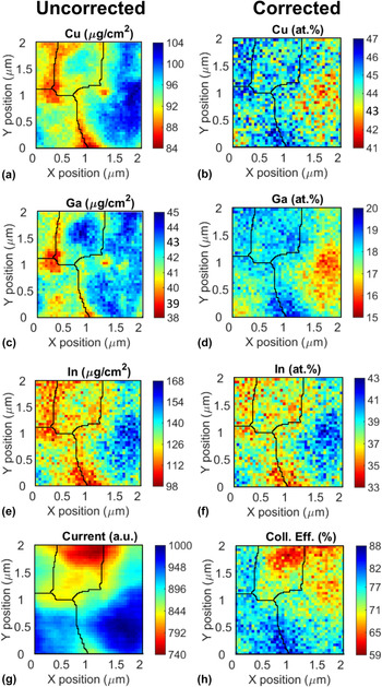
To demonstrate the effect of XRF and XBIC corrections to actual measurements and to emphasize the importance of applying data corrections, Fig. 10 shows XRF and XBIC maps of CIGS solar cells collected at beamline 26-ID-C of the Advanced Photon Source (APS) before and after attenuation and thickness corrections are applied (left: after step 2, right: after step 4 in Fig. 7). The left column shows the quantified but uncorrected XRF data and current measured by XBIC in arbitrary units. The black lines on top of the image are the result of a watershed analysis used to identify grain boundaries. Reference Tsukahara, Mitrovic, Gajdosik, Margaritondo, Pournin, Ramaioli, Sage, Hwu, Unser and Liebling87 Significant changes are noticed between the uncorrected and corrected maps, namely the grain to the right of the map appears to have a high concentration of all elements. However, after corrections it becomes evident that the grain is indium rich. All maps appear more pixelated after correction, which is due to the low signal-to-noise ratio of the indium channel. Atomic percentages were calculated as [X]/([Cu] + [In] + [Ga]), where X is the element of interest. Additionally, in the raw XBIC image it appears that the bottom left and right grain cores have the highest current but after correction, the intersecting boundary between the two has the highest collection efficiency.
2 × 2 μm2 XRF/XBIC maps measured with 50 nm step size and 1 s dwell time. Left column: Quantified uncorrected XRF and XBIC maps measured on a CIGS solar cell. Right column: Data corrected for self-attenuation, variations in beam absorption, and thickness variations. Using these corrections, elemental distributions can be converted from areal concentrations to atomic percent (here, 100% is defined as the sum of the cations Cu, Ga, and In without Se), and the current can be converted into charge collection efficiency for known incident photon flux. Black lines are the result of a watershed analysis performed on the uncorrected XRF data and indicate CIGS grain boundaries.

C. Toward integrative corrections
Although the corrections described in the previous section are important for a variety of XRF and XBIC measurements of solar cells, they are too simplistic for other applications. For example, the assumption of negligible lateral composition variations cannot be sustained in cases as in Fig. 16, where the iodine and lead concentrations vary by more than a factor of 2 at the micrometer scale. The fact that the preconditions of such corrections are not satisfied is acknowledged and discussed in Ref. Reference Stuckelberger, Nietzold, Hall, West, Werner, Niesen, Ballif, Rose, Fenning and Bertoni65. However, the statements about charge collection efficiency and its relation to the lead/iodine ratio remain valid, as they are based uniquely on the relative changes within a map.
Nevertheless, better correction algorithms are needed, not only for the quantitative evaluation of measurements of perovskite solar cells on a mesoporous scaffold as in Fig. 16, but for a wide variety of applications. With solar cell efficiencies approaching their theoretical limits, the improvement of light management gets more important, which translates into solar cell architectures with a larger ratio of surface roughness/absorber layer thickness. But properly quantified XRF data are needed beyond solar cell applications to account for incident and fluorescence photons passing through multiple domains, and it is even more critical for X-ray fluorescence tomography.
We are not aware of broadly available user-friendly correction algorithms that satisfy these needs. However, there are different approaches that could be used: a first approach is based on the utilization of spatially resolved information about the measured sample from different measurements. This approach is particularly interesting for correlative microscopy, where the use of different measurement parameters is not limited to output correlation but where the output from one measurement channel can serve as input for data correction of another measurement channel too. Examples of measurements of spatially resolved layer thicknesses that could provide the experimental fundament for pixel-by-pixel XRF correction include X-ray transmittance or tomography, surface-sensitive techniques such as atomic-force microscopy, or optical measurements such as Raman, photoluminescence, or LBIC.
Alternatively, we suggest an approach that relies on the XRF mapping itself only: based on the uncorrected map, a correction factor is determined at each pixel from its raw compositional data. This correction factor is applied, again pixel-by-pixel, to the original map. For a layer stack with known layer sequence, the corrected map is translated into a topological map. Based on this topological map, a second correction-factor map can be determined, taking into account for each pixel 3D information from other parts of the map, according to the known path of incident X-ray and excident X-ray fluorescence photons. Further iterations may follow until the iterations converge. For improvement of the uniqueness and accuracy of the result from this iterative approach, it could obviously be combined with the first approach.
IV. ADVANCED APPLICATIONS OF CORRELATIVE X-RAY MICROSCOPY
In the first subsection, we highlight achievements of correlative X-ray microscopy for mc-Si during the last 15 years. In the following subsections, we showcase further research projects reported during the last two years that apply correlative X-ray microscopy to solar cells and demonstrate the high pace of the developments in this field.
A. Crystalline silicon solar cells: the advent of defect engineering
While the detection of transition metal impurities in silicon-based matrixes dates to the early 1960s Reference Meyer88 it was not until the late 1990s that it was first used to study the distribution of metal precipitates in silicon and its correlation to minority carrier recombination measured by techniques like LBIC and EBIC. Reference McHugo, Thompson, Flink, Weber, Lamble, Gunion, MacDowell, Celestre, Padmore and Hussain89,Reference McHugo, Thompson, Mohammed, Lamble, Périchaud, Martinuzzi, Werner, Rinio, Koch, Hoefs and Haessler90 In a review of the effect of iron and its complexes on silicon device performance, Istatov et al. proposed synchrotron-based XRF as an emerging characterization method with high spatial resolution and sensitivity. Reference Istratov, Hieslmair and Weber91 Since then, X-ray microscopy of this X-ray transparent matrix has been instrumental in the understanding of the behavior of transition metal impurities in silicon-based solar cells. The correlation of XRF with X-ray absorption helped reveal the chemical state of the nanoscale precipitates that usually riddle mc-Si, Reference Buonassisi, Heuer, Vyvenko, Istratov, Weber, Cai, Lai, Ciszek and Schindler15,Reference Buonassisi, Istratov, Heuer, Marcus, Jonczyk, Isenberg, Lai, Cai, Heald, Warta, Schindler, Willeke and Weber92,Reference Buonassisi, Marcus, Istratov, Heuer, Ciszek, Lai, Cai and Weber93 which has served as a platform to multiple diffusion and gettering models.
The complementary use of XRF and multiple laser as well as electron beam based techniques has allowed to directly correlate the metal content at various types of mc-Si grain boundaries and dislocations. Buonassisi et al. showed that metal precipitation tends to vary inversely with the degree of atomic coincidence in the grain boundary plane Reference Buonassisi, Istratov, Pickett, Marcus, Ciszek and Weber94 and Bertoni et al. showed that recombination-active dislocations contain a high amount of nanometer-sized metallic particles, while recombination-inactive dislocations present no metal impurity decoration above the detection limits. Reference Bertoni, Fenning, Rinio, Rose, Holt, Maser and Buonassisi10
The development of XBIC (see Sec. II.A) opened the door to correlate one-to-one the precipitate location, chemical nature, and recombination activity. Reference Buonassisi, Heuer, Vyvenko, Istratov, Weber, Cai, Lai, Ciszek and Schindler15,Reference Vyvenko, Buonassisi, Istratov and Weber17,Reference Vyvenko, Buonassisi, Istratov, Hieslmair, Thompson, Schindler and Weber34,Reference Vyvenko, Buonassisi, Istratov, Weber, Kittler and Seifert47 Spectrally resolved X-ray beam-induced current was later introduced as a technique to locally probe the diffusion length around particular precipitates. Imaging of the same precipitate at different incident X-ray energies allows for the comparison of carrier collection efficiency and attenuation coefficient resulting in diffusion length. Reference Buonassisi, Istratov, Pickett, Marcus, Hahn, Riepe, Isenberg, Warta, Willeke, Ciszek and Weber16,Reference Buonassisi, Istratov, Marcus, Heuer, Pickett, Lai, Cai, Heald and Weber95
This type of analysis has allowed to effectively quantify the purity and compare the impurity distribution throughout multiple silicon sources, ingots, wafers and feedstock. Reference Bernardis, Newman, Di Sabatino, Fakra, Bertoni, Fenning, Larsen and Buonassisi13,Reference Trushin, Seifert, Vyvenko, Bauer, Martinez-Criado, Salome and Kittler40,Reference Istratov, Buonassisi, McDonald, Smith, Schindler, Rand, Kalejs and Weber96,Reference Buonassisi, Istratov, Pickett, Rakotoniaina, Breitenstein, Marcus, Heald and Weber97 It has also been instrumental in understanding the evolution of these impurities throughout processing. A study by Buonassisi et al. on the behavior of metallic precipitates during rapid thermal processing (RTP) showed for the first time the potential of this technique as a powerful guide for process optimization. Reference Buonassisi, Istratov, Peters, Ballif, Isenberg, Riepe, Warta, Schindler, Willeke, Cai, Lai and Weber98 That report showed that a short period of time at high-temperature RTP favors the dissolution of copper and nickel precipitates over iron nanoprecipitates. It also presented for the first time the idea that rapid cooling “freezes” the precipitates in smaller and more distributed recombination centers, leading to a decrease in solar cell performance. The concept of defect engineering was presented and it was based on the fact that the material’s performance is limited primarily by the distribution of the defects and not only by the total defect concentration. Reference Buonassisi, Istratov, Marcus, Lai, Cai, Heald and Weber11 These findings have driven significant advances in crystal growth and performance improvements in heavily contaminated materials. Reference Seifert, Vyvenko, Arguirov, Kittler, Salome, Seibt and Trushin45,Reference Buonassisi, Istratov, Pickett, Heuer, Kalejs, Hahn, Marcus, Lai, Cai, Heald, Ciszek, Clark, Cunningham, Gabor, Jonczyk, Narayanan, Sauar and Weber99 For example, Bernardini et al. recently tracked the evolution of photoluminescence (PL) active regions at different stages of the solar cells processing. Reference Bernardini, Johnston, West, Lai, Naerland, Stuckelberger and Bertoni18 The report explains the variation of sub-band-gap PL signal intensity variations happening during the antireflective coating by the variation of the small metal precipitates spatial density.
The observation of mixed-metal silicide co-precipitation via a liquid–alloy intermediate phase Reference Buonassisi, Heuer, Istratov, Pickett, Marcus, Lai, Cai, Heald and Weber100 inspired the first in situ measurement of metallic impurities in crystalline silicon using a modified Linkam stage. Reference Hudelson, Newman, Bernardis, Fenning, Bertoni, Marcus, Fakra, Lai and Buonassisi101 The results provided insight into the complex and fascinating nature of precipitate formation, segregation, and the counter intuitive phenomenon known as retrograde melting. Reference Hudelson, Newman, Bernardis, Fenning, Bertoni, Marcus, Fakra, Lai and Buonassisi101,Reference Fenning, Newman, Bertoni, Hudelson, Bernardis, Marcus, Fakra and Buonassisi102 This opened yet another door into defect engineering—the ability to evaluate the kinetics of processes.
One could argue that the combination of all these learnings with advanced kinetics models has been one of the single most powerful examples of how understanding the behavior of defects at the nanoscale can be used to drive industrially relevant process optimization. Reference Hofstetter, Fenning, Bertoni, Lelievre, Del Canizo and Buonassisi66,Reference Fenning, Hofstetter, Bertoni, Hudelson, Rinio, Lelievre, Lai, Del Canizo and Buonassisi103–Reference Haarahiltunen, Savin, Yli-Koski, Talvitie, Asghar and Sinkkonen105 The so-called impurity-to-efficiency calculator (I2E), which is an open source platform, allows one to calculate final solar cell performance as a function of the as-grown iron content and distribution in the Si wafer, the time–temperature profiles during solar cell processing, and the device architecture. Reference Hofstetter, Fenning, Bertoni, Lelievre, Del Canizo and Buonassisi66,Reference Fenning, Hofstetter, Bertoni, Hudelson, Rinio, Lelievre, Lai, Del Canizo and Buonassisi103 The particular process of P-diffusion and gettering has benefited tremendously from these developments, establishing very strong guidelines of time and temperature profiles for the mitigation of the limiting defect by precipitate dissolution and bulk removal for a variety of elements such as iron Reference Fenning, Hofstetter, Bertoni, Coletti, Lai, Del Canizo and Buonassisi106–Reference Hofstetter, Fenning, Powell, Morishige, Wagner and Buonassisi108 or chromium, Reference Jensen, Hofstetter, Morishige, Coletti, Lai, Fenning and Buonassisi109 or specifically to n-type silicon. Reference Morishige, Jensen, Hofstetter, Yen, Wang, Lai, Fenning and Buonassisi12
B. CIGS solar cells: effect of grain boundaries and elemental distribution on charge collection efficiency
The first statistically significant application of correlative X-ray microscopy to thin-film solar cells that utilizes combined operando measurements of XRF and XBIC is reported in Ref. Reference West, Stuckelberger, Guthrey, Chen, Lai, Maser, Rose, Shafarman, Al-Jassim and Bertoni61. Utilizing the nanoprobe beamline 26-ID-C at APS, XRF and XBIC maps of CIGS solar cells were obtained at the incident photon energy of 10.5 keV, just above the GaK edge for maximum sensitivity to the cations Ga, In, and Cu similar to the maps shown in Fig. 10. Two different samples were analyzed with different [Ga]/[In + Ga] (GGI) ratios: the device with GGI = 30% had a solar energy conversion efficiency of 18%, the device with GGI = 60% had an efficiency of 14%. For the separate analysis of regions in the bulk of CIGS crystallites and of regions that stood under the direct influence of grain boundaries, a watershed analysis was performed on the XRF maps, which were shown to correlate with maps obtained from backscattered electrons measured by scanning electron microscopy. This justified the use of watershed analysis for the identification of grain boundaries in CIGS absorber layers from XRF measurements. The further analysis identified grain-boundary regions as a band of 400 nm on either side of the grain boundary, accounting for the tilt of the sample during the measurements. Elemental composition and XBIC signal were corrected following the method described in Ref. Reference West, Stuckelberger, Jeffries, Gangam, Lai, Stripe, Maser, Rose, Vogt and Bertoni60.
For both regions, grain cores and grain boundaries, the corrected maps were correlated, pixel-by-pixel, with respect to charge collection efficiency and elemental distribution. An example of such a correlation between the Cu and In versus the charge collection efficiency is shown in Fig. 2. Of particular importance turned out to be the impact of the GGI and the ratio [Cu]/[In + Ga] (CGI) on charge collection efficiency. Figure 11 shows the fitted slope of CGI and GGI versus charge collection efficiency (XCE) at grain boundaries and grain cores for low and high gallium absorbers. Large slopes indicate that a greater change in composition is required to have an impact on the charge collection efficiency. The error bars correspond to the 95% confidence interval. The unfilled bars correspond to values below the detection limit for this analysis.
Slope of the fitted pixel-by-pixel correlation of the elemental ratios of [Cu]/[In + Ga] and [Ga]/[In + Ga] versus charge collection efficiency from the analysis of a multitude of maps that have been analyzed separately for regions around grain boundaries and grain cores for cells with different Ga content. Error bars indicated the 95% confidence intervals. Figure adapted from Ref. Reference West, Stuckelberger, Guthrey, Chen, Lai, Maser, Rose, Shafarman, Al-Jassim and Bertoni61. Reprinted from Nano Energy, Vol. 32, B.M. West, M. Stuckelberger, H. Guthrey, L. Chen, B. Lai, J. Maser, V. Rose, W. Shafarman, M. Al-Jassim, and M.I. Bertoni, Grain engineering: how inhomogeneities can control charge collection in solar cells, Vol. 32, Pages 488–493, Copyright (2017), with permission from Elsevier.

The analysis shows unambiguously that solar cells with low gallium absorbers have a stronger correlation between composition and collection efficiency than solar cells with high gallium absorbers. Furthermore, it can be seen in Fig. 11 that the charge collection efficiency in low gallium absorbers has a stronger dependence [smaller slope of d(at.%)/d(XCE)] on CGI and GGI at grain boundaries than at grain cores. The collection efficiency in low gallium solar cells also has overall a stronger dependence on GGI than CGI. For high gallium absorbers, a dependence of composition on collection efficiency was only detectable for the CGI in grain cores. No statistically meaningful dependence could be detected at grain boundaries or between GGI and XCE at grain cores. These analyses show how composition variations can have a positive impact on the charge collection efficiency at structural defects like grain boundaries. Additionally, they can be used to provide a path forward to improving solar cell growth parameters to favor beneficial composition changes and hinder detrimental ones.
C. CIGS solar cells: in situ growth of CuIn x Ga1−x Se2
The ability to measure and visualize film properties during growth allows for direct insight to how grains are formed, how temperature impacts elemental segregation/phase formation, and how quickly diffusion processes and ripening take place. It is necessary to understand the behavior of a material after growth, but it is even more powerful to understand how the material achieved these properties. In situ X-ray diffraction (XRD) has been highly useful to understand phase segregation during growth as a function of time and temperature. Reference Kim, Payzant, Yoon and Anderson110,Reference Mainz and Klenk111 A challenge with these data, however, is a lack of sufficient spatial resolution, and there is no clear insight into the process of phase formation. To fill this gap, a temperature and atmosphere controlled in situ stage was designed that can be installed at APS beamline 2-ID-D and is capable of measuring XRF at temperatures up to 600 °C at the spatial resolution of the beamline. Reference Chakraborty, Serdy, West, Stuckelberger, Lai, Maser, Bertoni, Culpepper and Buonassisi70
Using this in situ stage, West et al. Reference West, Stuckelberger, Chen, Lovelett, Lai, Maser and Bertoni77 have studied the growth of (Ag,Cu)(In,Ga)Se2 (ACIGS) films via a precursor reaction process as described in Ref. Reference Berg, Cheng and Shafarman112, measuring the time-dependent variation of the elemental distribution. The addition of Ag to CIGS films is interesting because of the band gap widening of CIGS without additional gallium incorporation (which would deteriorate the performance) and because of the lower melting point of ACIGS. Reference Chen, Lee and Shafarman113
Prior to the in situ experiment, metallic AgCuInGa precursor films were prepared by sequential sputtering of CuGa, In, and AgGa. The resulting film composition was [Ga]/[Ga + In] = 0.2, [Cu + Ag]/[In + Ga] = 0.82, and [Ag]/[Ag + Cu] = 0.28. Precursors were capped with 10 μm of evaporated selenium. Experiments were conducted at the APS beamline 2-ID-D above the GaK absorption edge (10.4 keV), to allow sufficient sensitivity to all cations; measurements above the SeK edge (12.7 keV) that would allow the assessment of all main constituents, suffer typically from low sensitivity to the InL lines. The beam full width half maximum (FWHM), limiting the spatial resolution for these measurements, was ∼150 nm.
The measured temperature profile is shown in Fig. 12(a) with the insets showing two examples of XRF maps. Compared to steady-state measurements as described in the previous section, time constraints are more severe during dynamic in situ experiments as reported here, which requires compromises with respect to sensitivity, mapped area, and spatial resolution. However, recent improvements of the detector sensitivity and count rate, as well as the development of flying-scan mode Reference Morishige, Laine, Jensen, Yen, Looney, Vogt, Lai, Savin and Buonassisi114 provided partial compensation.
(a): Heating profile during the in situ formation of (Ag,Cu)(In,Ga)Se2 (ACIGS) crystalline films from metallic precursors at sector 2-ID-D of the Advanced Photon Source at the Argonne National Laboratory. The insets show the Cu distribution measured after 73 and 175 min. (b): Change of the correlation coefficient of the major film constituents during the in situ annealing. Unconnected data points in the beginning and at the end correspond to room-temperature measurements.

Understanding how elements segregate with respect to one another by mapping them throughout the growth process gives unique insight into drivers for phase formation. One way to illustrate segregation is by calculating the correlation coefficient described by
 $$\rho \left( {A,B} \right) = {1 \over {N - 1}}\sum\limits_{i = 1}^N {\left( {{{\overline {{A_i} - {\mu _{\rm{A}}}} } \over {{\sigma _{\rm{A}}}}}} \right)\left( {{{\overline {{B_i} - {\mu _{\rm{B}}}} } \over {{\sigma _{\rm{B}}}}}} \right)}$$
with A and B being the two parameters whose correlation is of interest. N is the sample size, σ is the standard deviation of the data set, and μ is the sample mean. Correlation coefficients vary from −1 to 1, where −1 is a perfect negative correlation and 1 is a perfect positive correlation.
Figure 12(b) shows the change in correlation coefficients between Cu, In, Ga, and Ag in the ACIGS system during the formation of ACIGS from the metallic precursors. The unconnected data points in the beginning and at the end correspond to room-temperature measurements.
Cu and Ga show initially a strong positive correlation likely due to the co-sputtered CuGa precursor layer. With the initial heating, Cu and Ga exhibit a decreasing correlation until ∼100 min where these elements are no longer correlated, until after cooling. The positive correlation after cooling is likely due to topological effects, where thickness variations even of stoichiometric ACIGS leads to positive correlations.
While initially segregating together, Cu and In drift toward anti-correlation. Surprisingly, Ga and In show no correlation throughout the heating process even though they substitute one another in the CIGS lattice, which should lead to an anticorrelation for stoichiometric layers. Cu and Ag show a very strong positive correlation throughout the growth process, despite their substitutional nature and the fact that they were not co-deposited. It is possible that a Cu x Ag y alloy is formed during the growth process, but this would need validation by XRD measurements. In and Ag exhibit a strong negative correlation.
These results describe the first results of in situ formation of ACIGS crystallites with elemental mapping such as reported in Ref. Reference West, Stuckelberger, Chen, Lovelett, Lai, Maser and Bertoni77. Future experiments should include in situ X-ray diffraction studies to support the trends observed in this analysis, and the change in correlation coefficients over time may give insight into the rate of phase formation or even diffusion coefficients. An added benefit of in situ XRF studies is the ability to isolate individual particles such as demonstrated in Sec. IV.F for steady-state measurements of perovskite solar cells, and track how those change over time.
D. Organic solar cells: from crystallinity to phase separation for low Z elements
Organic photovoltaic (OPV) solar cells are interesting because of their potential to be very low cost, scalable, and compatible with high-throughput, roll-to-roll manufacturing processes. However, the low efficiencies achieved even for laboratory scale devices (the certified record efficiency is currently 11.2% Reference Green, Emery, Hishikawa, Warta, Dunlop, Levi and Ho-Baillie26 ) combined with poor reliability are a challenge, even though efficiencies have significantly improved in the last few years. Reference Jørgensen, Norrman, Gevorgyan, Tromholt, Andreasen and Krebs115,Reference Tanenbaum, Hermenau, Voroshazi, Lloyd, Galagan, Zimmermann, Hosel, Dam, Jørgensen, Gevorgyan, Kudret, Maes, Lutsen, Vanderzande, Wurfel, Andriessen, Rosch, Hoppe, Teran-Escobar, Lira-Cantu, Rivaton, Uzunoglu, Germack, Andreasen, Madsen, Norrman and Krebs116 Another challenge associated with OPV is a lack of understanding of the impact that phase separation and impurity concentration have on final device properties.
Throughout different types of organic solar cells, one of the most important, but least understood, properties is long-range crystallinity. Reference Collins, Tumbleston and Ade117 Until recently, however, existing techniques have been unable to probe non-crystalline orientations with high-resolution over large length scales. Therefore, the understanding of how to synthesize polymer films with a preferred orientation has been limited. Reference Collins, Cochran, Yan, Gann, Hub, Fink, Wang, Schuettfort, McNeill, Chabinyc and Ade118
It is not just crystallinity and morphology that are critical to these films; there is also the worry that contaminants from the catalyst used during synthesis are incorporated into the polymer matrix and negatively affect the device efficiency. Reference Nikiforov, Lai, Chen, Chen, Schaller, Strzalka, Maser and Darling119 Element-sensitive imaging with high spatial resolution is required to understand long-range ordering and impurity concentrations in polymer films.
Crystallinity in OPV films is often studied using either grazing incidence small-angle or wide-angle X-ray scattering (GISAXS or GIWAXS respectively). Each technique is able to identify both the crystallization and phase separation of films, and several beamlines offer in situ capabilities. Reference Collins, Tumbleston and Ade117 Using grazing incidence X-ray scattering, divergent conclusions have been formed on the role of poly(3-hexylthiophene) (P3HT) and phenyl-C61-butyric acid methyl ester (PCBM) in phase separation and crystallization in mixed polymers; while the existence of PCBM in P3HT films prohibits the crystallization of P3HT, it has been unclear whether, during annealing, crystallization competes with or drives phase separation of the two polymers. Reference Collins, Tumbleston and Ade117,Reference Agostinelli, Lilliu, Labram, Campoy-Quiles, Hampton, Pires, Rawle, Bikondoa, Bradley, Anthopoulos, Nelson and MacDonald120,Reference Lilliu, Agostinelli, Pires, Hampton, Nelson and MacDonald121
In addition to X-ray scattering, grazing incidence X-ray diffraction (GIXRD) has been used to determine the molecular ordering of PCBM-P3HT blends used in high efficiency devices, which consistently display face-on preferential packing orientation. Reference Beiley, Hoke, Noriega, Dacuña, Burkhard, Bartelt, Salleo, Toney and McGehee122,Reference Bartelt, Beiley, Hoke, Mateker, Douglas, Collins, Tumbleston, Graham, Amassian, Ade, Fréchet, Toney and McGhee123 Rivnay, et al. applied in situ GIXRD to observe a change in plane orientations upon heating and cooling the polymer P(NDI2OD-T2). Footnote l They found that face-on reflections completely disappeared near the melting temperature and were replaced with edge-on orientations. This behavior was also observed in other polymers, such as P3HT and P3HT blends. Reference Rivnay, Steyrleuthner, Jimison, Casadei, Chen, Toney, Facchetti, Neher and Salleo124
To further understand phase separation in mixed polymer organic solar cells, scanning transmission X-ray microscopy (STXM) combined with polarized soft X-rays scattering (P-SoXS) has been used, observing composition variations in the films. P-SoXS is unique from other techniques because it is able to quantitatively measure molecular orientation in the absence of long-range order with high resolution. Reference Collins, Cochran, Yan, Gann, Hub, Fink, Wang, Schuettfort, McNeill, Chabinyc and Ade118 Additionally, it has orders of magnitude better contrast than previously used methods, in turn requiring lower exposure dosage and thus limiting sample damage during measuring.
An example of the findings from STXM/P-SoXS is shown in Fig. 13. Dashed lines in Figs. 13(a) and 13(b) highlight the boundaries of two distinct domains. Whereas Fig. 13(a) was taken at 390 eV, where the image contrast is solely representative of mass-thickness differences, Fig. 13(b) was taken at 285.9 eV, where the measurement is sensitive to domain orientation. The authors interpret the larger features at lower energy as clustering of smaller, similarly oriented domains. Reference Collins, Cochran, Yan, Gann, Hub, Fink, Wang, Schuettfort, McNeill, Chabinyc and Ade118
Scanning transmission X-ray microscopy (STXM) images taken at two energies of incident X-rays, (a) 390 eV and (b) 285.9 eV. (a) is the energy for mass-thickness contrast whereas (b) is an energy that shows correlative domain orientation. Reprinted by permission from Macmillan Publishers Ltd: Nature Materials [B.A. Collins, J.E. Cochran, H. Yan, E. Gann, C. Hub, R. Fink, C. Wang, T. Schuettfort, C.R. McNeill, M.L. Chabinyc, and H. Ade: Polarized X-ray scattering reveals non-crystalline orientational ordering in organic films. Nat. Mater. 11(6), 536 (2012)], copyright (2012).

E. Nanowire solar cells: radial and longitudinal gradients
Nanowire solar cells show intrinsic advantages compared to other types of solar cells. Most importantly, they eliminate the trade-off between optically thick absorbers for high absorptance and electrically thin absorber layers for low recombination losses, as light is absorbed vertically but charge carriers are collected radially. However, the lack of low-cost manufacturing methods—often, nanowire fabrication relies on wafer substrates and utilizes precious metals—combined with moderate solar cell efficiencies have limited their wide-spread application so far.
Although a variety of material systems is being explored for nanowire solar cells, including hydrogenated amorphous silicon, Reference Qian, Misra, Lu, Yu, Yu, Xu, Wang, Xu, Shi, Chen and Cabarrocas125 MAPI perovskite, Reference Im, Luo, Franckevicius, Pellet, Gao, Moehl, Zakeeruddin, Nazeeruddin, Grätzel and Park126 InP, Reference Wallentin, Anttu, Asoli, Huffman, Aberg, Magnusson, Siefer, Fuss-Kailuweit, Dimroth, Witzigmann, Xu, Samuelson, Deppert, Borgström, Huynh, Dittmer, Alivisatos, O’Regan, Grätzel, Polman, Atwater, Mårtensson, Colombo, Heiβ, Grätzel, Fontcuberta i Morral, Wang, Gudiksen, Duan, Cui, Lieber, Borgström, Garnett, Brongersma, Cui, McGehee, Goto, Kupec, Stoop, Witzigmann, Hu, Chen, Anttu, Xu, Kelzenberg, Garnett, Yang, Green, Emery, Hishikawa, Warta, Dunlop, Borgström, Mårtensson, Anttu, Xu, Wu, Anttu, Xu, Samuelson, Pistol, Münch, Joyce, Mishra, van Weert, Yella, Ip, Popov, Nevière, Gralak, Tayeb, Jellison and Modine127 or GaAs, Reference Parkinson, Lee, Fu, Breuer, Tan and Jagadish128,Reference Krogstrup, Jørgensen, Heiss, Demichel, Holm, Aagesen, Nygard and Fontcuberta i Morral129 we focus here on the findings from correlative X-ray microscopy on In x Ga1−x N nanowire solar cells.
J. Segura-Ruiz and G. Martínez-Criado, et al. made use of complementary X-ray techniques at the nanoprobe station ID22NI at the European Synchrotron Radiation Facility (ESRN) to analyze In x Ga1−x N nanowires combining XRF, XRD, and X-ray absorption near edge spectroscopy (XANES) at the nanoscale. Reference Segura-Ruiz, Martínez-Criado, Denker, Malindretos and Rizzi130–Reference Martínez-Criado, Homs, Alén, Sans, Segura-Ruiz, Molina-Sanchez, Susini, Yoo and Yi133
Through XRF, elemental distributions were evaluated within the In x Ga1−x N nanowires and Ga was found to be unevenly distributed both longitudinally as well as radially as shown in Fig. 14. Whereas the nanowire core is In-rich throughout the length of the nanowire, the peripheral regions gradually fade from In-rich in the top part (left in the longitudinal view image in Fig. 14) toward Ga-rich in the bottom part. The authors suggest that the formation of parasitic Ga-rich outer regions are caused by the low processing temperatures that limit the growth of GaN nanocolumns.
Indium and gallium distributions in an In x Ga1−x N nanowire. Top (longitudinal view): relative In and Ga concentrations are estimated from X-ray fluorescence measurements. Bottom (radial view): In (left) and Ga (right) distributions of two In x Ga1−x N nanowires on a silicon substrate in top view. Reprinted (adapted) with permission from Ref. Reference Segura-Ruiz, Martínez-Criado, Denker, Malindretos and Rizzi130, J. Segura-Ruiz, G. Martínez-Criado, C. Denker, J. Malindretos, and A. Rizzi: Phase separation in single In x Ga1−x N nanowires revealed through a hard X-ray synchrotron nanoprobe. Nano Lett. 14, 1300 (2014). Copyright (2014) American Chemical Society.

The long-range order of the nanowires was assessed through XRD that was measured simultaneously with XRF. Qualitatively in agreement with the compositional variations indicated by the XRF measurements, three XRD peaks were identified at the bottom of the nanowires indicating different alloys, whereas only one peak was visible at the top where the compositional map indicates pure InN.
Additional XANES measurements at the InK edge support these findings further and suggest that the tetrahedral structure within the nanowires is maintained throughout, despite the compositional variations. However, peak broadening is observed compared to a reference spectrum for InN, suggesting that there is reduced long-range order within the In x Ga1−x N nanowires. Reference Segura-Ruiz, Martínez-Criado, Chu, Denker, Malindretos and Rizzi131
Exemplarily utilizing a variety of X-ray techniques, Martínez-Criado, et al. studied nanowires consisting of a ZnO core and an outer In x Ga1−x N/GaN multishell structure by X-ray excited optical luminescence (XEOL) to assess the optical performance of the nanowires in addition to composition and structure by XRF/XRD. Reference Martínez-Criado, Segura-Ruiz, Alén, Eymery, Rogalev, Tucoulou and Homs132,Reference Martínez-Criado, Homs, Alén, Sans, Segura-Ruiz, Molina-Sanchez, Susini, Yoo and Yi133 Specifically, XEOL made it possible to probe the quantum confinement predicted for such structures and to extract the carrier diffusion length that was found to be lower than reported earlier, suggesting increased mobility-limiting scattering in the fabricated nanowires.
Comparing the XEOL spectra with predictions of the quantum confinement, an energy-shift could be experimentally confirmed and the authors found that the wave function confinement occurs preferentially in the corners of the hexagonal nanowire cross section. Moreover, a negative relationship was found between the quantum well dimension and intensity of the confinement effect. Reference Martínez-Criado, Homs, Alén, Sans, Segura-Ruiz, Molina-Sanchez, Susini, Yoo and Yi133 This conclusion was evaluated against the elemental segregation observed in the XRF images to prove that the confinement was not caused by variation in chemical composition. Through analyzing the XRF image, it was found that indium segregation is negligible and thus the best explanation for the XEOL results is the one-dimensional confinement effect. Reference Martínez-Criado, Segura-Ruiz, Alén, Eymery, Rogalev, Tucoulou and Homs132
Beyond these examples of In x Ga1−x N/GaN nanowires, research on semiconductor nanowires has been significantly advanced by correlative X-ray microscopy at nanoprobe hard X-ray beamlines as demonstrated by the variety of material systems, including Co-ZnO Reference Martínez-Criado, Segura-Ruiz, Alén, Eymery, Rogalev, Tucoulou and Homs132,Reference Chu, Martínez-Criado, Segura-Ruiz, Geburt and Ronning134,Reference Chu, Martínez-Criado, Segura-Ruiz, Geburt and Ronning135 or ZnS Reference Rosenberg, Shenoy, Heigl, Lee, Kim, Zhou and Sham136 nanowires that have been studied by XRF, XANES, XRD, and XEOL.
F. Perovskite solar cells: compositional inhomogeneities at the nanoscale
High-resolution synchrotron X-ray fluorescence has been used to study the elemental dispersion within perovskite solar cells. In particular, mixed organic–inorganic perovskites consisting of the widely used MAPI have been shown to incorporate chlorine into the matrix, even when the samples are synthesized using nominally chlorine-free precursors. For identifying minute chlorine concentrations, X-ray fluorescence has proven to be an effective tool used for both qualitative and quantitative analyses.
For example, Unger et al. analyzed mixed halide perovskites synthesized using the precursors methylammonium iodide and lead chloride. Reference Unger, Bowring, Tassone, Pool, Gold-Parker, Cheacharoen, Stone, Hoke, Toney and McGehee137 To evaluate the concentration of chlorine remaining after various amounts of annealing time at 95°C, XRF and X-ray photoelectron spectroscopy (XPS) were used. The XRF data demonstrated that after 120 min of annealing, chlorine was still detectable, while XPS could not detect chlorine anymore. This highlights one of the benefits of applying XRF to perovskite solar cells: the bulk sensitivity of this technique makes it less sensitive to surface modifications of that highly unstable material.
Further studies by Luo et al. Reference Luo, Gamliel, Nijem, Aharon, Holt, Stripe, Rose, Bertoni, Etgar and Fenning25 have sought to identify the degree of chlorine incorporation using different precursors. Their samples were fabricated using five different precursor combinations, three of which contained chlorine and two that were nominally chlorine-free. They were analyzed using synchrotron-based XRF using sector 26-ID-C at APS. The high sensitivity and ability to probe the entire absorber layer made it possible to identify trace quantities of chlorine even in samples synthesized with chlorine-free precursors. The study implemented a similar attenuation correction to that described in Ref. Reference West, Stuckelberger, Jeffries, Gangam, Lai, Stripe, Maser, Rose, Vogt and Bertoni60 and Sec. III.B, taking into account attenuation losses both of the incident and excident beam through the sample layers. Unlike the qualitative analysis performed by Unger et al., Reference Unger, Bowring, Tassone, Pool, Gold-Parker, Cheacharoen, Stone, Hoke, Toney and McGehee137 which looked at relative peak intensity changes to form conclusions solely on the declining presence of chlorine within annealed samples, the work by Luo et al. quantified the chlorine concentration in each sample, measuring the spatial distribution of chlorine within a 2D map. For example, ratios of 0.0012 to 0.0058 Cl/I were reported using the technique, highlighting the degree of sensitivity of quantitative nano-XRF.
This provided important information on the extent of chlorine infiltration per synthesis conditions. In particular, it verified the hypothesis that the quantities of chlorine incorporated in the matrix directly relate to the amount of chlorine present in the synthesis precursors. Secondly, the high resolution capabilities of the nano-XRF enabled the demonstration of the preferential placement of chlorine near or along crystal grain boundaries. The segregation of elements near the grain boundaries has been shown to result in differing effects on electrical performance. Thus, applying correlative XRF/XBIC approaches on such chlorine-incorporated samples would further elucidate the effect that chlorine presence has on device performance of mixed halide perovskites.
In addition to the Cl/I ratio, the inhomogeneity of the chlorine incorporation throughout the layer was investigated in Ref. Reference Luo, Gamliel, Nijem, Aharon, Holt, Stripe, Rose, Bertoni, Etgar and Fenning25. Deeper analysis was done by implementing the built-in watershed method in MATLAB to evaluate heterogeneity within individual perovskite particles and amongst different particles. Figure 15 exemplifies the results of this procedure, where we note a distinct variation of chlorine concentration within individual particles. In addition to the qualitative comparison of the maps, the histograms demonstrate the inconsistency of chlorine concentration throughout the highlighted particles. The proximity of high-concentration and low-concentration regions visually represent the clustering of chlorine, possibly due to high flexibility in the bulk chemistry of the perovskite material. These observations on the degree of incorporation and how it relates to synthesis environments and procedures provides the opportunity to enhance growth methods and manipulate elemental incorporation for band gap and defect engineering of the material.
High-resolution maps showing the distribution of iodine (I), chlorine (Cl), and their ratio in randomly selected areas of a solar cell with a perovskite absorber layer. The absorber layer was deposited from the precursors PbI2, CH3NH3I (methylammonium iodide, MAI), and CH3NH3Cl (methylammonium chloride, MACl) with a ratio MAI/MACl = 1. Reprinted (adapted) with permission from Ref. Reference Luo, Gamliel, Nijem, Aharon, Holt, Stripe, Rose, Bertoni, Etgar and Fenning25, Y. Luo, S. Gamliel, S. Nijem, S. Aharon, M. Holt, B. Stripe, V. Rose, M.I. Bertoni, L. Etgar, and D.P. Fenning: Heterogeneous chlorine incorporation in organic–inorganic perovskite solar cells. Chem. Mater. 28(18), 6536 (2016). Copyright 2016 American Chemical Society.

G. Perovskite solar cells: charge collection efficiency on mesoporous scaffold
The report by Stuckelberger, et al. demonstrates for the first time correlative XBIC/XRF measurements of perovskite solar cells. Reference Stuckelberger, Nietzold, Hall, West, Werner, Niesen, Ballif, Rose, Fenning and Bertoni65 The solar cells with a MAPI absorber layer used for this experiment were synthesized by the process described in Ref. Reference Werner, Dubuis, Walter, Löper, Moon, Nicolay, Morales-Masis, De Wolf, Niesen and Ballif138. Deposited on glass with indium tin-oxide as transparent conductive oxide (TCO), a mesoporous TiO2 scaffold intermixed with the MAPI absorber layer sits on top of a compact TiO2 layer acting as electron transport layer (ETL). On the rear side, a spiro-MeOTAD layer acts as the hole transport layer (HTL) and is covered with a TCO for the potential application of using the cell as a top cell in tandem devices.
The combined XRF/XBIC measurements were performed at the APS beamline 26-ID-C using an excitation energy of 9 keV to measure the IL and the PbM lines of the perovskite absorber. The beam-spot size was approximately 40 nm FWHM. The resulting XRF data was fitted and corrected for self-absorption following the workflow described in Sec. III. These corrections are critical, as they assume minimal surface roughness and uniformity within each layer; only in this case, the attenuation of incident and outgoing X-ray photons can be calculated from tabulated X-ray attenuation coefficients following the method described above. Yet, applying these corrections yields more accurate results than not applying them.
Figure 16 shows such corrected maps measured under the same conditions and on the same sample as reported in Refs. Reference Stuckelberger, Nietzold, Hall, West, Werner, Ballif, Rose, Fenning and Bertoni64 and Reference Stuckelberger, Nietzold, Hall, West, Werner, Niesen, Ballif, Rose, Fenning and Bertoni65. Similarly to the procedure shown in those references, the XBIC measurement was performed prior to the XRF measurements due to a particular challenge of perovskite solar cells: they are sensitive to degradation caused by the high flux density of the X-ray beam. A noticeable decay in the XBIC signal was observed when measured coincidently with XRF. Fortunately, the sensitivity of XBIC is high enough and the electrical response of both, the charge collection process inside the solar cell and the read-out electronics, is fast enough, such that accelerated XBIC measurements under reduced beam intensity permit the acquisition while minimizing the X-ray beam induced degradation. The attentive reader will notice that the step size of the XBIC measurement was enhanced compared to the XRF measurement; this made the degradation corrections of the XBIC measurement that are discussed in Ref. Reference Stuckelberger, Nietzold, Hall, West, Werner, Niesen, Ballif, Rose, Fenning and Bertoni65 obsolete for the measurements presented here. Note that the degradation of the electrical performance is orders of magnitude faster and more dramatic than compositional degradation. Reference Stuckelberger, Nietzold, Hall, West, Meng, Werner, Niesen, Lai, Maser, Rose, Ballif and Bertoni139 Therefore, XRF measurements are not significantly affected by X-ray beam induced degradation.
Elemental distribution of iodine, lead, and their atomic ratio from X-ray fluorescence, and X-ray beam induced current (XBIC) measurement from the same area of a perovskite solar cell with a methylammonium lead iodide absorber layer on a mesoporous titanium oxide scaffold; the structure of this solar cell is shown in Fig. 3. The compositional maps are corrected for attenuation of the incident X-rays by layers on top of the absorber layer, and for attenuation of the exciting fluorescence photons. The XBIC measurement is corrected for beam attenuation by the layers on top of the absorber layer, and for thickness variations of the absorber layer itself such that the map corresponds to a collection efficiency. The black lines are the result of a watershed analysis Reference Gütay, Lienau and Bauer21 applied to the iodine map, separating regions of high iodine concentration, i.e., thick absorber layer.

One of the key benefits of nanoscale XRF is the ability to recognize relative elemental distributions. In the case of perovskite solar cells, which are well-known for their tendency to react with the atmosphere, XRF provides the opportunity to analyze the stoichiometric changes throughout the solar cell. In the absorber layer, we expect a relative distribution of Pb/I = 1/3 consistently within apparent grains, should the MAPI perovskite absorber layer have stoichiometric lead-to-iodine distribution.
From the comparison of the fluorescence signal to the current in Fig. 16, we note a correlation between the stoichiometry of the absorber layer and the charge collection efficiency. This type of analysis offers the ability to detect different phases at nanoscale and to understand how chemical composition variations impact the charge collection efficiency in different regions—be it between grains and grain boundaries similar to the analysis of CIGS presented in Sec. IV.B, or between bulk perovskite and the TiO2/perovskite interface that is critical for charge collection. Specifically, it has been shown that grain boundaries in the perovskite absorber result in reduced electrical performance in comparison to within the grains, providing recombination centers. Reference Yun, Ho-Baillie, Huang, Woo, Heo, Seidel, Huang, Cheng and Green23,Reference Leblebici, Leppert, Li, Reyes-Lillo, Wickenburg, Wong, Lee, Melli, Ziegler, Angell, Ogletree, Ashby, Toma, Neaton, Sharp and Weber-Bargioni140
Whereas the stoichiometric ratio of Pb/I in MAPI is mostly met in Fig. 16, there is a spot around coordinates (X, Y) = (−1.5 µm/−0.5 µm) with significantly larger ratio of nearly 1/2. This could indicate the occurrence of the PbI2 phase there, which is known to be a degradation product. Indeed, the comparison with the XBIC signal at that spot yields locally poor solar cell performance. Note that the occurrence of a large Pb/I ratio and low XBIC signal specifically at this spot rather than over the entire map indicates an issue of the solar cell that is not related to the measurement itself.
It is emphasized in Ref. Reference Stuckelberger, Nietzold, Hall, West, Werner, Niesen, Ballif, Rose, Fenning and Bertoni65 that the correction algorithms are not yet fully developed, and additional corrections and thorough 3D simulations need to be performed for a higher accuracy of quantified elemental distributions and charge collection efficiency. Nevertheless, we would like to point out that correlative X-ray microscopy methods combining XBIC with XRF can yield already valuable results as demonstrated in Ref. Reference Stuckelberger, Nietzold, Hall, West, Werner, Niesen, Ballif, Rose, Fenning and Bertoni65 and here, in spite of challenging measurement corrections of perovskite solar cells that are highly non-uniform both vertically and horizontally, and in spite of measurement-induced degradation that need to be taken into account.
V. THE FUTURE OF IN SITU AND OPERANDO CORRELATIVE X-RAY MICROSCOPY
Most of the results and techniques showcased in this article would not have been possible a few years ago, mainly due to limitations of photon flux and spatial resolution. Advances in accelerator and beamline science, optics, mirrors, detectors, stages and experimental hardware in general have enabled the presented in situ and operando studies. We are certain that this is just the beginning of a new era in synchrotron-based experiments and correlated microscopy in general, not only for functional materials but also for devices.
Future beamline upgrades contemplate smaller spot size, higher energy resolution, higher coherence, and longer working distance. Whereas new beamlines such as the HXN beamline at NSLS II approach limits set by physical laws in terms of spatial resolution, Reference Nazaretski, Xu, Bouet, Zhou, Yan, Huang and Chu141,Reference Chu, Yan, Nazaretski, Kalbfleisch, Huang, Lauer and Bouet142 the limits in working distance are rather of financial and technological nature. A description of how future nanoprobe in situ and operando beamlines could look like is presented in Ref. Reference Maser, Lai, Buonassisi, Cai, Chen, Finney, Gleber, Jacobsen, Preissner, Roehrig, Rose, Shu, Vine and Vogt143. From the experimental point of view, the working distance in the range of 5 cm rather than few hundred micrometers we have today is crucial: this will open the door to new plug-and-play in situ approaches, as not only different gas atmospheres, but portable reactors and film deposition stages could be implemented without the need of building an entire beamline around a deposition chamber as it is the case today. The additional space allows for the installation of measurement equipment in parallel for complementary X-ray characterization techniques such as synchrotron X-ray scanning tunneling microscopy. Reference Cummings, Chien, Preissner, Madhavan, Diesing, Bode, Freeland and Rose144,Reference Shirato, Cummings, Kersell, Li, Stripe, Rosenmann, Hla and Rose145
The further development of experimental methods—enabled by the strong coherence of the probing X-ray beam—contributes significantly to further progress: techniques like coherent diffraction imaging (CDI) Reference Yang, Huang, Harder, Clark, Robinson and Mao146 or ptychography Reference Dierolf, Menzel, Thibault, Schneider, Kewish, Wepf, Bunk and Pfeiffer147 not only enable spatial resolution below the spot size, but the phase information will add a whole new dimension to the data. This will enhance time-resolved measurements, or provide otherwise inaccessible information about the strain and stress inside of crystallites. In particular, Bragg CDI has become a mature technique in the last few years: applications have been successfully demonstrated for operando measurements of cathode nanoparticles in batteries, Reference Ulvestad, Singer, Clark, Cho, Kim, Harder, Maser, Meng and Shpyrko148 in situ measurements of Pd nanoparticles during the hydriding phase transformation Reference Ulvestad, Welland, Cha, Liu, Kim, Harder, Maxey, Clark, Highland, You, Zapol, Hruszkewycz and Stephenson149 and of Ag nanoparticles during the voltage-induced electrochemical dissolution. Reference Liu, Lopes, Cha, Harder, Maser, Maxey, Highland, Markovic, Hruszkewycz, Stephenson, You and Ulvestad150
The increase in brilliance that future lightsource upgrades will provide, Reference Einfeld151 allows for dramatically faster measurements, not only enabling higher sample throughput but more importantly permitting the measurement of new dimensions: with short dwell times, not only 3D absorption but also fluorescence tomography become reasonable, and instead of either compositional (XRF) or chemical (EXAFS) measurements, energy scans of each pixel of a compositional map are within reach. Then, X-ray diffraction pattern or synchrotron based deep-level transient spectroscopy (DLTS) can be performed at each point of an inhomogeneous sample with nanoscale resolution. In a way, it is like solving the material’s paradigm, structure-properties-processing and performance relationship for every nanoscale voxel (volumetric pixel) of the specimen under study.
These exciting new opportunities come with new challenges: with the increase of measured dimensions, the absorbed dose in a sample increases dramatically, which is even more of a concern for operando measurements of electronic devices such as solar cells, as the performance is typically affected more from locally generated electric defects than the elemental distribution.
Similarly, the thermal load can become an issue—not only on the X-ray optics but also on samples. In situ and operando experiments often exacerbate this issue, as they add energy to the sample (e.g., from bias light or bias voltage for solar cells), leading to further temperature increase particularly if the experimental chamber is kept under vacuum.
The biggest challenge, however, is without a doubt the incredible amount of data that will be generated. Development of better and faster readout electronics, data transfer, storage, and computing capabilities is a technical challenge, but more challenging is the development of algorithms to help read, process and analyze these data. For example, the 3D reconstruction of crystallites from CDI scans is feasible today for exemplary crystals, typically isolated gold particles. Scientifically of more interest are crystallites embedded in their environment such as in operational solar cells. However, there are not yet reconstruction algorithms available that are robust enough to deal with complex data. Another example of this are in situ experiments such as the one presented in Sec. IV.C: procedures to correct such data for self-absorption and to compensate for thermal drift of structures being modified are just being developed. More importantly though, algorithms that can help visualize and track trends and changes will be of the utmost importance. This is a recurring problem that multiple fields face, with huge computational efforts being necessary to extract the maximum information hidden in the newly accessible dimensions of space, phase, energy, time, and environmental parameters. Solar cell research could really benefit from in situ and operando approaches and machine learning developments could take this science to an entirely new level.
ACKNOWLEDGMENTS
We greatly acknowledge Jérémie Werner, Bjoern Niesen, Christophe Ballif (all EPFL, Switzerland), Harvey Guthrey, Mowafak Al-Jassim (all NREL, USA), Lei Chen, William Shafarman (all U. of Delaware, USA) for providing solar cells; Rupak Chakraborty, Jim Serdy, Tonio Buonassisi (all MIT, USA) for their contributions building the heating stage, David Fenning (UC San Diego, USA) for fruitful discussions, Chris Roehrig and Martin Holt (both ANL, USA) for practical help with XBIC measurements, Yanqi Luo (UC San Diego, USA) for measurement of the PbI2 reference, and Genevieve Hall, Sebastian Husein, Srikanth Gangam, and April Jeffries (all ASU, USA) for their contribution to measurements and discussions.
We acknowledge funding from the U.S. Department of Energy under contract DEEE0005848. Use of the Center for Nanoscale Materials and the Advanced Photon Source, both Office of Science user facilities, was supported by the U.S. Department of Energy, Office of Science, Office of Basic Energy Sciences, under Contract No. DE-AC02-06CH11357. This material is based upon work supported in part by the National Science Foundation (NSF) and the Department of Energy (DOE) under NSF CA No. EEC-1041895. Any opinions, findings and conclusions or recommendations expressed in this material are those of the author(s) and do not necessarily reflect those of NSF or DOE.