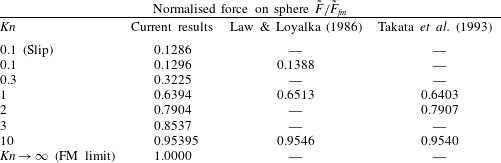
1 Introduction
Modern nanoelectromechanical devices have dimensions ranging from tens to hundreds of nanometres (Tzou, Beraun & Chen Reference Tzou, Beraun and Chen2002; Ekinci & Roukes Reference Ekinci and Roukes2005; Jensen, Kim & Zettl Reference Jensen, Kim and Zettl2008; Pelton et al. Reference Pelton, Sader, Burgin, Liu, Guyot-sionnest and Gosztola2009; O’Connell et al. Reference O’Connell, Hofheinz, Ansmann, Bialczak, Lenander, Lucero, Neeley, Sank, Wang, Weides, Wenner, Martinis and Cleland2010). These devices often generate gas flows whose characteristic length scale, such as the device size, is comparable to the mean free path of the gas. A continuum treatment of such gas flows does not properly account for their underlying physics – a more advanced theoretical framework is required. Importantly, continuum theory is strictly valid only in the limit of vanishing Knudsen number,
 $$\begin{eqnarray}Kn\equiv \frac{{\it\lambda}}{L_{c}},\end{eqnarray}$$
where
 ${\it\lambda}$
is the gas mean free path and
 $L_{c}$
is a characteristic length scale of the flow; this can be related to the gas viscosity (Sharipov & Seleznev Reference Sharipov and Seleznev1998). For steady flows, the Knudsen number can be used to distinguish different flow regimes. Near-continuum flows result when
 $Kn\ll 1$
, and these can be analysed using the Navier–Stokes equations with no-slip or slip boundary conditions (Cercignani Reference Cercignani2000) – interparticle collisions in the gas dominate particle/wall collisions, and thus the gas is in a state of near equilibrium. Flows that exhibit a large Knudsen number (
 $Kn\gg 1$
) have minimal interparticle collisions and can be studied using the collisionless Boltzmann equation – the gas distribution function deviates strongly from the (equilibrium) Maxwell–Boltzmann distribution. In this free-molecular case, gas–surface interactions dominate the flow which is strongly non-local (Cercignani Reference Cercignani2000). The stress at any position in space depends implicitly on all other spatial positions, and the (continuum) concept of a stress tensor that is dependent only on the local velocity gradient does not apply. In contrast, flows with
 $Kn\sim O(1)$
are often said to be in a transition regime, because interparticle collisions and particle collisions with a solid boundary occur with similar frequency, and are thus equally important processes.
Unsteady gas flows are also characterised by the Knudsen number and, in addition, depend on the frequency ratio,
 $$\begin{eqnarray}{\it\Theta}\equiv \frac{{\it\omega}_{c}}{{\it\nu}},\end{eqnarray}$$
where
 ${\it\omega}_{c}$
is a characteristic angular oscillation frequency of the flow and
 ${\it\nu}$
is an interparticle collision frequency of the gas, which can be expressed in terms of its viscosity (Sharipov & Kalempa Reference Sharipov and Kalempa2007). For
 ${\it\Theta}\ll 1$
, many interparticle collisions occur within one oscillation period of the flow, whereas very few collisions occur when
 ${\it\Theta}\gg 1$
(Sharipov & Kalempa Reference Sharipov and Kalempa2007, Reference Sharipov and Kalempa2008). The Knudsen number,
 $Kn$
, and frequency ratio,
 ${\it\Theta}$
, are thus two distinct parameters that non-dimensionalise all unsteady flows.
Nanomechanical devices such as doubly clamped carbon nanotube beams (Jensen et al. Reference Jensen, Kim and Zettl2008), nanocantilever sensors (Li, Tang & Roukes Reference Li, Tang and Roukes2007) and metal nanoparticles (Pelton et al. Reference Pelton, Sader, Burgin, Liu, Guyot-sionnest and Gosztola2009) are often driven at their natural resonant frequencies. When operated under ambient conditions, i.e. in air, they inherently generate unsteady (time-dependent) rarefied gas flows. These nanoscale systems can easily be operated at frequencies in the gigahertz range (Pelton et al. Reference Pelton, Chakraborty, Malachosky, Guyot-Sionnest and Sader2013), which is comparable to the interparticle collision frequency of air molecules at standard temperature and pressure. This exacerbates deviations from an equilibrium (Maxwell–Boltzmann) distribution which already exist due to operation at finite Knudsen number – thus further violating a key assumption of continuum theory. Gas flows induced by such nanoscale systems therefore cannot be studied using classical continuum theory, i.e. the Navier–Stokes equations.
Continuum theory can only be formally applied when
 $Kn\ll 1$
and
 ${\it\Theta}\ll 1$
. A statistical mechanical treatment of the gas is typically used for flows outside this range. This yields the Boltzmann equation for a dilute gas, which is valid for all Knudsen numbers and frequency ratios. Particle interactions in the gas are described by the collision term of the Boltzmann equation, which complicates analysis due to its multidimensional integral form (for a real gas). To alleviate this mathematical issue, the collision term is often replaced by a relaxation operator that mimics the behaviour of a real gas. This model was proposed independently by Bhatnagar, Gross & Krook (Reference Bhatnagar, Gross and Krook1954) and Welander (Reference Welander1954), and is commonly referred to as the BGK kinetic model. It involves the approximation of interparticle collisions by a relaxation process with a time constant,
 $1/{\it\nu}$
. The resulting Boltzmann–BGK equation has been used extensively to study a variety of rarefied gas flows (Cercignani Reference Cercignani2000; Sone Reference Sone2002). Despite its well-known shortcomings, e.g. the Prandtl number differs from that of a real monatomic gas, the BGK kinetic model has provided significant insight into rarefied gas flows and produces good quantitative agreement with more realistic collision integrals, such as that for a hard-sphere gas (Sharipov & Seleznev Reference Sharipov and Seleznev1998).
In recent years, there has been considerable progress in understanding the effects of unsteadiness on rarefied gas flows. This body of work has been motivated by the abovementioned technological advances in the design, fabrication and application of nanomechanical devices. These include unidirectional flows such as pulsating Poiseuille flow (Hansen & Ottesen Reference Hansen and Ottesen2006; Taheri et al. Reference Taheri, Rana, Torrilhon and Struchtrup2009), oscillatory Couette flow (Sharipov & Kalempa Reference Sharipov and Kalempa2008; Taheri et al. Reference Taheri, Rana, Torrilhon and Struchtrup2009; Yap & Sader Reference Yap and Sader2012), Stokes’ second problem for the in-plane oscillation of a flat plate in contact with an unbounded gas (Sharipov & Kalempa Reference Sharipov and Kalempa2007; Gu & Emerson Reference Gu and Emerson2011) and unsteady thermal flows (Manela & Hadjiconstantinou Reference Manela and Hadjiconstantinou2008, Reference Manela and Hadjiconstantinou2010; Nassios & Sader Reference Nassios and Sader2012, Reference Nassios and Sader2013).
Despite this activity, the unsteady flow generated by an oscillating sphere in an unbounded rarefied gas is yet to be explored. This provides the primary motivation and focus of the present article. The only study to report a solution to this problem is a computational study by Ladiges & Sader (Reference Ladiges and Sader2015), for the singular case of
 $Kn=1$
and
 ${\it\Theta}=1$
. This previous study was performed using both time-domain and frequency-domain Monte Carlo methods, and was limited to a single case due to the computational expense involved in simulating a three-dimensional flow. Here, we provide a complete analysis of this canonical problem over a wide range of
 $Kn$
and
 ${\it\Theta}$
, and explore the underlying physics of this flow. This not only provides important benchmark data for future numerical and analytical studies, but also enables a range of applications that involve oscillations of spheres in rarefied gases to be properly understood and characterised, e.g. the electromagnetic trapping of a nanoparticle in a gas (Neukirch et al.
Reference Neukirch, Gieseler, Quidant, Novotny and Vamivakas2013).
The effects of unsteadiness in the low-Knudsen-number regime have been recently explored using asymptotic analyses of the Boltzmann equation, in both the low-frequency (Nassios & Sader Reference Nassios and Sader2012; Takata & Hattori Reference Takata and Hattori2012) and high-frequency (Nassios & Sader Reference Nassios and Sader2013) limits. These studies show that unsteadiness can dramatically affect the transport equations and boundary conditions for the flow. At low frequency, for example, gas rarefaction modifies the momentum transport equation at first order in the Knudsen number, resulting in an additional unsteady body force that depends on the imposed temperature gradient. That is, the governing equation for the bulk flow away from any boundary is not the (continuum) unsteady Stokes equation, for a thermally driven flow. Furthermore, unsteadiness and heat transport couple strongly at both first and second orders in the Knudsen number. This is of particular relevance to the oscillation of a sphere in a rarefied gas, since the flow is inherently non-isothermal; see below.
The drag on a sphere moving with steady uniform velocity in an unbounded viscous (continuum) fluid was solved by Stokes in the 19th century (Stokes Reference Stokes1880). The impact of this classical result on scientific and technological advancement has been widespread, with countless applications making use of the formula for Stokes drag, including the Stokes–Einstein equation for diffusion of a sphere in a viscous fluid (Einstein Reference Einstein1905; Sutherland Reference Sutherland1905).
Shortly after its publication, it was observed that Stokes drag does not accurately predict the drag on a sphere in a slightly rarefied gas flow, e.g. that of a particle of radius 0.005 mm (Millikan Reference Millikan1923). Early theoretical attempts to resolve this discrepancy derived approximate asymptotic solutions, for both small and large Knudsen numbers (Cunningham Reference Cunningham1910; Epstein Reference Epstein1923; Baker & Charwat Reference Baker and Charwat1958; Phillips Reference Phillips1975). These analyses were facilitated by the original experimental measurements, which were performed over a wide range of Knudsen numbers (Millikan Reference Millikan1923). Later theoretical studies employed the BGK kinetic model (Liu, Pang & Jew Reference Liu, Pang and Jew1965; Willis Reference Willis1966), and made use of the method of Knudsen iteration, to obtain asymptotic solutions in the near free-molecular regime. Asymptotic solutions for small Knudsen number were also obtained using a matched asymptotic expansion (Sone & Aoki Reference Sone, Aoki and Potter1976) and the R13 moment method (Torrilhon Reference Torrilhon2010). Other approaches valid for all Knudsen numbers were explored, including the variational method (Cercignani & Pagani Reference Cercignani and Pagani1968; Cercignani, Pagani & Bassanini Reference Cercignani, Pagani and Bassanini1968), direct finite differencing of the Boltzmann equation (Lea & Loyalka Reference Lea and Loyalka1982; Law & Loyalka Reference Law and Loyalka1986) and the direct simulation Monte Carlo (DSMC) method (Chun & Koch Reference Chun and Koch2005; Nourazar & Ganjaei Reference Nourazar and Ganjaei2010). Collision terms in the Boltzmann equation, such as the BGK model, that for a hard-sphere gas and variable hard spheres, have all been studied.
A comprehensive numerical data set is available for the steady flow past a sphere, according to the hard-sphere linearised Boltzmann equation – radial and angular components of the bulk velocity, the density, temperature and drag are reported up to four decimal places (Takata, Sone & Aoki Reference Takata, Sone and Aoki1993). Tabular data for the linearised Boltzmann–BGK equation are also available. Under the assumption that the flow is isothermal, Lea & Loyalka (Reference Lea and Loyalka1982) provided radial and angular components of the bulk velocity, the density and the drag up to four decimal places. Results for the non-isothermal case were also published later by Law & Loyalka (Reference Law and Loyalka1986), again to four decimal places. The studies by Lea & Loyalka (Reference Lea and Loyalka1982) and Law & Loyalka (Reference Law and Loyalka1986) report slightly different density profiles for isothermal flow. In addition, separate drag results for the Boltzmann–BGK equation obtained by finite differencing and the variational method are also available (again to four decimal places), both with the isothermal assumption (Cercignani et al. Reference Cercignani, Pagani and Bassanini1968) and without the isothermal assumption (Takata et al. Reference Takata, Sone and Aoki1993). Importantly, while previous works made a distinction between isothermal and non-isothermal flows around a sphere, only the latter formally applies because the impact of gas particles at a solid wall at normal incidence always generates a temperature jump (away from the continuum limit) (Sone Reference Sone2002). This induces a non-isothermal flow throughout the gas, even for low Mach number, i.e. where the linearised Boltzmann equation is valid.
The unsteady problem, i.e. flow driven by an oscillating sphere in an unbounded fluid, has been studied extensively in the continuum limit. The solution to the linear problem was also derived by Stokes (Reference Stokes1880), while Riley (Reference Riley1966) studied a slightly unsteady flow for a continuum fluid using a matched asymptotic expansion. Flow in the continuum regime at finite Reynolds number, i.e. finite oscillation amplitude, has also been studied by Mei & Adrian (Reference Mei and Adrian1992) and Mei (Reference Mei1994), who compared finite-difference numerical solutions of the Navier–Stokes equations with an asymptotic analytical solution. While the unsteady flow generated by an oscillating sphere in the continuum limit has been explored extensively, the effect of gas rarefaction on this flow has not been studied. This article explores this outstanding problem in detail, and in so doing also provides comprehensive numerical solutions for the density, temperature, velocity profile and force on the sphere. These solutions are used to elucidate the physical mechanisms driving the flow and study the combined effects of unsteadiness and gas rarefaction.
The article is organised as follows. We commence in § 2 by presenting the theoretical formulation, which includes the problem statement and derivation of a set of coupled integral equations from the Boltzmann–BGK equation. An expression for the force on the sphere is also derived in terms of the bulk velocity, density and temperature of the gas. This is followed in § 3 by derivation and discussion of analytical solutions in various asymptotic limits. Details of the numerical methods for arbitrary degrees of gas rarefaction are discussed separately in § 4, for both steady and unsteady flows – data from the former are used for verification with available literature results, whereas the latter provide new results. In § 5, numerical results for both steady and unsteady flows are presented, together with a discussion of the underlying physical mechanisms in each flow. For unsteady flow, we provide full numerical profiles for the bulk gas velocity in the radial and angular directions, density and temperature. Tabular data for the force on the sphere for both steady and unsteady flows are also provided, which are expected to be of value in practical applications.
2 Theoretical formulation
The motion of a sphere of radius
 $a$
in a gas is considered, where the sphere velocity is either (i) constant (steady) or (ii) oscillatory (unsteady). The gas flow induced by the sphere motion obeys the Boltzmann–BGK equation, a particle conservation equation valid for all Knudsen numbers and oscillation frequencies:
 $$\begin{eqnarray}\frac{\partial F}{\partial t}+\boldsymbol{c}\boldsymbol{\cdot }\frac{\partial F}{\partial \boldsymbol{x}}+\boldsymbol{a}\boldsymbol{\cdot }\frac{\partial F}{\partial \boldsymbol{c}}={\it\nu}({\it\rho}f^{M}-F),\end{eqnarray}$$
where
 $$\begin{eqnarray}f^{M}(\boldsymbol{x},\boldsymbol{c},t)=\left(\frac{m}{2{\rm\pi}kT(\boldsymbol{x},t)}\right)^{3/2}\exp \left(-\frac{m|\boldsymbol{c}-\boldsymbol{U}(\boldsymbol{x},t)|^{2}}{2kT(\boldsymbol{x},t)}\right).\end{eqnarray}$$
In (2.1) and (2.2),
 $F$
is the mass distribution function of the gas,
 $\boldsymbol{x}$
is the spatial coordinate,
 $\boldsymbol{c}$
is the gas particle velocity,
 $t$
is time,
 $k$
is Boltzmann’s constant,
 $m$
is the molecular mass of the gas,
 $\boldsymbol{a}$
is an external force per unit mass,
 ${\it\rho}(\boldsymbol{x},t)$
is the gas density,
 ${\it\nu}$
is an interparticle collision frequency and
 $f^{M}$
is the local Maxwell–Boltzmann distribution function with temperature
 $T$
and bulk velocity
 $\boldsymbol{U}$
. The surface of the sphere provides a diffuse boundary condition for the gas particles, and the temperature of the sphere is identical to that of the free-stream gas.
The velocity of the sphere is much smaller than the most probable speed of gas particles. This permits linearisation of the Boltzmann–BGK equation, where the mass distribution function
 $F$
is expanded as
 $$\begin{eqnarray}F(\boldsymbol{x},\boldsymbol{c},t)={\it\rho}_{0}\left(\frac{m}{2{\rm\pi}kT_{0}}\right)^{3/2}\exp \left(-\frac{m}{2kT_{0}}|\boldsymbol{c}|^{2}\right)\left(1+\frac{U_{0}}{c_{m}}h(\boldsymbol{x},\boldsymbol{c},t)\right),\end{eqnarray}$$
giving corresponding expressions for the density and temperature
 $$\begin{eqnarray}\displaystyle \displaystyle {\it\rho}(\boldsymbol{x},t) & \hspace{-2.0pt}=\hspace{-2.0pt} & \displaystyle {\it\rho}_{0}\left(1+\frac{U_{0}}{c_{m}}w(\boldsymbol{x},t)\right),\end{eqnarray}$$
 $$\begin{eqnarray}\displaystyle \displaystyle T(\boldsymbol{x},t) & \hspace{-2.0pt}=\hspace{-2.0pt} & \displaystyle T_{0}\left(1+\frac{U_{0}}{c_{m}}{\it\tau}(\boldsymbol{x},t)\right),\end{eqnarray}$$
 $h$
is the perturbation distribution function,
 ${\it\rho}_{0}$
is the equilibrium density,
 $T_{0}$
is the equilibrium temperature,
 $w$
is the density perturbation,
 ${\it\tau}$
is the temperature perturbation,
 $c_{m}=\sqrt{2kT_{0}/m}$
is the most probable speed of gas particles and
 $U_{0}$
is the velocity amplitude of the sphere; see figure 1. The interparticle collision frequency
 ${\it\nu}$
is constant in this linear limit. Substituting (2.3) and (2.4) into (2.1), and scaling appropriately, yields the required dimensionless linearised equation for the gas flow,
 $$\begin{eqnarray}\frac{{\it\Theta}}{Kn}\frac{\partial h}{\partial t}+\boldsymbol{c}\boldsymbol{\cdot }\frac{\partial h}{\partial \boldsymbol{x}}=\frac{1}{Kn}\left(w+2\boldsymbol{c}\boldsymbol{\cdot }\boldsymbol{U}+\left[|\boldsymbol{c}|^{2}-\frac{3}{2}\right]{\it\tau}-h\right),\end{eqnarray}$$
where the following set of scales has been used: (i) distance is scaled by the sphere radius,
 $a$
, (ii) gas particle velocities are scaled by the most probable speed,
 $c_{m}$
, (iii) bulk gas velocity is scaled by the velocity amplitude of the sphere,
 $U_{0}$
, (iv) time is scaled by the reciprocal of the oscillation frequency of the sphere,
 ${\it\omega}^{-1}$
, and (v) gas temperature and density perturbations are scaled by
 $U_{0}/c_{m}$
. All variables are henceforth dimensionless.
The Knudsen number
 $Kn\equiv {\it\lambda}/a$
and frequency ratio
 ${\it\Theta}\equiv {\it\omega}/{\it\nu}$
arise naturally, where
 ${\it\omega}$
is the angular oscillation frequency of the sphere,
 ${\it\nu}$
is the gas collision frequency and
 ${\it\lambda}$
is the gas mean free path. Equation (2.5) is formally valid in the asymptotic low-speed limit,
 $U_{0}\ll c_{m}$
, i.e. infinitesimal Mach number.
Without loss of generality, we study the unsteady (oscillatory) problem first, where the scaled sphere velocity is
 $\boldsymbol{U}_{sp}=\text{Re}\{\exp (-\text{i}t)\}\hat{\boldsymbol{z}}=\text{Re}\{[\cos {\it\theta}\hat{\boldsymbol{r}}-\sin {\it\theta}\hat{{\bf\theta}}]\exp (-\text{i}\text{t})\}$
and
 $(r,{\it\theta},{\it\phi})$
are the usual spherical coordinates; see figure 1. As discussed, the resulting gas flow is controlled by the Knudsen number and the frequency ratio. Another dimensionless parameter that is commonly used to capture unsteady effects is the inverse Stokes number,
 ${\it\beta}\equiv (a/{\it\delta})^{2}$
, where
 ${\it\delta}=\sqrt{2{\it\mu}/({\it\rho}_{0}{\it\omega})}$
is the viscous penetration depth and
 ${\it\mu}$
is the shear viscosity of the gas. However, there are only two independent parameters in the flow, since
 ${\it\Theta}=Kn^{2}{\it\beta}$
(Yap & Sader Reference Yap and Sader2012). Flow generated by a sphere moving with constant velocity,
 $U_{0}$
, i.e. the steady problem, is obtained by setting
 ${\it\omega}=0$
, or, equivalently,
 ${\it\Theta}=0$
. This steady problem has been studied widely, e.g. see Cercignani et al. (Reference Cercignani, Pagani and Bassanini1968), Lea & Loyalka (Reference Lea and Loyalka1982), Law & Loyalka (Reference Law and Loyalka1986), Takata et al. (Reference Takata, Sone and Aoki1993), Chun & Koch (Reference Chun and Koch2005), Nourazar & Ganjaei (Reference Nourazar and Ganjaei2010) and Torrilhon (Reference Torrilhon2010).
Schematic of a sphere of radius
 $a$
, showing the Cartesian coordinate system; the origin is at the centre of the sphere. The sphere velocity is in the
 $z$
direction, and oscillates with amplitude
 $U_{0}$
and angular frequency
 ${\it\omega}$
. It should be noted that Re refers to the real component, and all listed variables here are dimensional.

All time-varying functions are expressed in terms of the time dependence:
 $$\begin{eqnarray}Z=\text{Re}\{\tilde{Z}\exp (-\text{i}t)\},\end{eqnarray}$$
where
 $Z\in \{h,w,\boldsymbol{U},{\it\tau},\boldsymbol{U}_{sp}\}$
, the operator ‘
 $\text{Re}$
’ refers to the real component and the ‘
 $\,\tilde{\,}\,$
’ notation represents the spatial component of the function. Equation (2.5) then becomes
 $$\begin{eqnarray}\frac{1-\text{i}{\it\Theta}}{Kn}\tilde{h}+\boldsymbol{c}\boldsymbol{\cdot }\frac{\partial \tilde{h}}{\partial \boldsymbol{x}}=\frac{1}{Kn}\left(\tilde{w}+2\boldsymbol{c}\boldsymbol{\cdot }\tilde{\boldsymbol{U}}+\left[|\boldsymbol{c}|^{2}-\frac{3}{2}\right]\tilde{{\it\tau}}\right).\end{eqnarray}$$
We use the approach of Cercignani & Pagani (Reference Cercignani and Pagani1966) and Lea & Loyalka (Reference Lea and Loyalka1982) to formulate integral equations from (2.7). These integral equations are obtained by integrating along the characteristics of (2.7), which are a family of straight lines in the direction of the particle velocity,
 $\boldsymbol{c}$
, namely
 $$\begin{eqnarray}\boldsymbol{x}(q)=\frac{\boldsymbol{c}}{V}q+\boldsymbol{C},\end{eqnarray}$$
where
 $V=|\boldsymbol{c}|$
is the magnitude of the particle velocity vector and
 $\boldsymbol{C}\in \mathbb{R}^{3}$
is a constant vector.
Schematic of a characteristic along the line spanning the particle velocity
 $\boldsymbol{c}$
that passes through the position
 $\boldsymbol{x}$
and a point
 $\boldsymbol{x}_{0}$
on the sphere surface. Here,
 $\hat{\boldsymbol{r}}$
,
 $\hat{{\bf\theta}}$
and
 $\hat{{\bf\phi}}$
are unit vectors in the radial, polar angle and azimuthal directions respectively at the position
 $\boldsymbol{x}$
(upper right point). The black dots (top to bottom) indicate the following positions: (1)
 $\boldsymbol{x}$
, an arbitrary position in the gas; (2)
 $\boldsymbol{x}^{\prime }$
, an arbitrary position lying on the characteristic; (3)
 $\boldsymbol{x}_{0}$
, the position on the surface of the sphere; and (4) the origin,
 $\boldsymbol{O}$
, which coincides with the centre of the sphere. Characteristics lying outside the dashed lines do not intersect the sphere. The distance
 $s$
is from
 $\boldsymbol{x}$
to
 $\boldsymbol{x}^{\prime }$
. The particle velocity,
 $\boldsymbol{c}$
, is expressed in its spherical coordinates
 $(V,{\it\chi},{\it\psi})$
, where
 $V=|\boldsymbol{c}|$
and the angles
 ${\it\chi}$
and
 ${\it\psi}$
are illustrated; see (2.9).

Figure 2 shows a schematic of a characteristic passing through an arbitrary position,
 $\boldsymbol{x}$
, and a point on the sphere surface,
 $\boldsymbol{x}_{0}$
, along the line spanned by the direction,
 $\boldsymbol{c}$
. The spherical coordinate of position
 $\boldsymbol{x}$
is
 $(r,{\it\theta},{\it\phi})$
and the spherical coordinate of position
 $\boldsymbol{x}^{\prime }$
, a point on the characteristic, is
 $(r^{\prime },{\it\theta}^{\prime },{\it\phi}^{\prime })$
, as indicated in figure 2. For a given position in the gas,
 $\boldsymbol{x}$
, the family of characteristics comprises all possible straight lines between
 $\boldsymbol{x}$
and the sphere surface that do not pass through the interior of the sphere, i.e. they intersect the sphere surface on the side facing the point
 $\boldsymbol{x}$
.
The molecular velocity
 $\boldsymbol{c}=c_{r}\hat{\boldsymbol{r}}+c_{{\it\theta}}\hat{{\bf\theta}}+c_{{\it\phi}}\hat{{\bf\phi}}$
in (2.7) and (2.8) can be written in terms of its spherical coordinates,
 $(V,{\it\chi},{\it\psi})$
, i.e.
 $$\begin{eqnarray}\displaystyle & \displaystyle c_{r}=V\cos {\it\chi}, & \displaystyle\end{eqnarray}$$
 $$\begin{eqnarray}\displaystyle & \displaystyle c_{{\it\theta}}=V\sin {\it\chi}\sin {\it\psi}, & \displaystyle\end{eqnarray}$$
 $$\begin{eqnarray}\displaystyle & \displaystyle c_{{\it\phi}}=V\sin {\it\chi}\cos {\it\psi}, & \displaystyle\end{eqnarray}$$
 $V=|\boldsymbol{c}|$
is the magnitude of the particle velocity,
 ${\it\chi}$
is the angle between the radial unit vector
 $\hat{\boldsymbol{r}}$
and the particle velocity vector
 $\boldsymbol{c}$
, and
 ${\it\psi}$
is the angle between the azimuthal unit vector
 $\hat{{\bf\phi}}$
and the projection of
 $\boldsymbol{c}$
on the
 ${\it\theta}$
–
 ${\it\phi}$
plane; see figure 2. From (2.8), it follows that
 $$\begin{eqnarray}\boldsymbol{c}\boldsymbol{\cdot }\frac{\partial \tilde{h}}{\partial \boldsymbol{x}}=V\frac{\partial \tilde{h}}{\partial q}.\end{eqnarray}$$
Substituting (2.10) into (2.7), and using an integrating factor, we obtain
 $$\begin{eqnarray}\tilde{h}\exp \left(\frac{1-\text{i}{\it\Theta}}{Kn}\frac{q}{V}\right)=\int _{0}^{q}\frac{1}{VKn}\left(\tilde{w}+2\boldsymbol{c}\boldsymbol{\cdot }\tilde{\boldsymbol{U}}+\left[|\boldsymbol{c}|^{2}-\frac{3}{2}\right]\tilde{{\it\tau}}\right)\exp \left(\frac{1-\text{i}{\it\Theta}}{Kn}\frac{q^{\prime }}{V}\right)\,\text{d}q^{\prime }+D.\end{eqnarray}$$
The constant
 $D$
is determined by applying the scaled and linearised boundary conditions,
 $$\begin{eqnarray}\displaystyle & \displaystyle \lim _{|\boldsymbol{x}-\boldsymbol{x}_{0}|\rightarrow \infty }\tilde{h}(\boldsymbol{x},\boldsymbol{c})=0, & \displaystyle\end{eqnarray}$$
 $$\begin{eqnarray}\displaystyle & \displaystyle \tilde{h}(\boldsymbol{x}_{0},\boldsymbol{c})=2\boldsymbol{c}\boldsymbol{\cdot }\tilde{\boldsymbol{U}}_{sp}+\sqrt{{\rm\pi}}\tilde{\boldsymbol{U}}_{sp}\boldsymbol{\cdot }\hat{\boldsymbol{r}}-\frac{2}{{\rm\pi}}\int _{\boldsymbol{c}\boldsymbol{\cdot }\hat{\boldsymbol{r}}<0}\exp (-|\boldsymbol{c}|^{2})(\boldsymbol{c}\boldsymbol{\cdot }\hat{\boldsymbol{r}})\tilde{h}(\boldsymbol{x}_{0},\boldsymbol{c})\,\text{d}\boldsymbol{c},\quad \boldsymbol{c}\boldsymbol{\cdot }\hat{\boldsymbol{r}}>0, & \displaystyle \nonumber\\ \displaystyle & & \displaystyle\end{eqnarray}$$
 $\boldsymbol{x}_{0}$
is a position vector on the sphere surface and
 $\tilde{\boldsymbol{U}}_{sp}$
is the scaled velocity of the sphere. Equation (2.12a
) is the free-stream condition far from the surface of the sphere, whereas (2.12b
) is the linearised diffuse boundary condition at the sphere surface.
Application of the boundary conditions in (2.12) to (2.11) gives the required expression for
 $\tilde{h}(\boldsymbol{x},\boldsymbol{c})$
, which is discontinuous in particle velocity space:
 $$\begin{eqnarray}\displaystyle & & \displaystyle \tilde{h}(\boldsymbol{x},\boldsymbol{c})=\left\{\begin{array}{@{}ll@{}}\begin{array}{@{}l@{}}\displaystyle \int _{0}^{|\boldsymbol{x}-\boldsymbol{x}_{0}|}\frac{1}{VKn}\left(\tilde{w}(\boldsymbol{x}^{\prime })+2c_{r^{\prime }}\tilde{U} _{r^{\prime }}(\boldsymbol{x}^{\prime })+2c_{{\it\theta}^{\prime }}\tilde{U} _{{\it\theta}^{\prime }}(\boldsymbol{x}^{\prime })+\left[V^{2}-\frac{3}{2}\right]\tilde{{\it\tau}}(\boldsymbol{x}^{\prime })\right)\\ \displaystyle \quad \times \,\exp \left(-\frac{1-\text{i}{\it\Theta}}{VKn}|\boldsymbol{x}-\boldsymbol{x}^{\prime }|\right)\,\text{d}|\boldsymbol{x}-\boldsymbol{x}^{\prime }|\\ \displaystyle \quad +\,\tilde{h}_{0}(\boldsymbol{x}_{0},\boldsymbol{c})\exp \left(-\frac{1-\text{i}{\it\Theta}}{VKn}|\boldsymbol{x}-\boldsymbol{x}_{0}|\right),\quad \boldsymbol{c}\in R1,\end{array}\quad \\ \begin{array}{@{}l@{}}\displaystyle \int _{0}^{\infty }\frac{1}{VKn}\left(\tilde{w}(\boldsymbol{x}^{\prime })+2c_{r^{\prime }}\tilde{U} _{r^{\prime }}(\boldsymbol{x}^{\prime })+2c_{{\it\theta}^{\prime }}\tilde{U} _{{\it\theta}^{\prime }}(\boldsymbol{x}^{\prime })+\left[V^{2}-\frac{3}{2}\right]\tilde{{\it\tau}}(\boldsymbol{x}^{\prime })\right)\\ \quad \times \displaystyle \exp \left(-\frac{1-\text{i}{\it\Theta}}{VKn}|\boldsymbol{x}-\boldsymbol{x}^{\prime }|\right)\,\text{d}|\boldsymbol{x}-\boldsymbol{x}^{\prime }|,\quad \boldsymbol{c}\in R2,\end{array}\quad & \end{array}\right.\end{eqnarray}$$
where all symbols are defined in figure 2, and
 $c_{i}$
,
 $U_{i}$
are components of the molecular velocity
 $\boldsymbol{c}$
and bulk velocity
 $\boldsymbol{U}$
in the
 $i$
direction in spherical coordinates respectively. The domains
 $R1$
and
 $R2$
are
 $$\begin{eqnarray}\displaystyle \left.\begin{array}{@{}c@{}}\displaystyle R1:\quad V\in [0,\infty ),\quad {\it\chi}\in [0,\arcsin (1/r)],\quad {\it\psi}\in [0,2{\rm\pi}],\\ \displaystyle R2:\quad V\in [0,\infty ),\quad {\it\chi}\in [\arcsin (1/r),{\rm\pi}],\quad {\it\psi}\in [0,2{\rm\pi}],\end{array}\right\} & & \displaystyle\end{eqnarray}$$
and
 $$\begin{eqnarray}\tilde{h}_{0}(\boldsymbol{x}_{0},\boldsymbol{c})=2\boldsymbol{c}\boldsymbol{\cdot }\tilde{\boldsymbol{U}}_{sp}+\sqrt{{\rm\pi}}\tilde{\boldsymbol{U}}_{sp}\boldsymbol{\cdot }\hat{\boldsymbol{r}}-\frac{2}{{\rm\pi}}\int _{c_{r}<0}\exp (-|\boldsymbol{c}|^{2})c_{r}\tilde{h}(\boldsymbol{x}_{0},\boldsymbol{c})\,\text{d}\boldsymbol{c},\quad \boldsymbol{c}\in R1.\end{eqnarray}$$
The regions of particle velocity space,
 $R1$
and
 $R2$
, in (2.14) are shown schematically in figure 3(a); red line arrows correspond to the region
 $R1$
and green line arrows are in the region
 $R2$
.
(a) Particle velocity space. Red arrows are velocity directions contained within region
 $R1$
, whose surface is a cone with apex at
 $\boldsymbol{x}$
; all velocities in this region point away from the sphere. Green arrows are all velocity directions not contained in
 $R1$
– this corresponds to
 $R2$
; see (2.14). (b) Integration regions given an arbitrary position
 $\boldsymbol{x}$
. Here,
 $A0$
is the region containing points that do not have direct line of sight to
 $\boldsymbol{x}$
, i.e. a line joining a point in this region to
 $\boldsymbol{x}$
must pass through the sphere;
 $A1$
is the region containing all lines emanating from the hemispherical surface of the sphere facing
 $\boldsymbol{x}$
that pass through
 $\boldsymbol{x}$
; the boundaries of this region are tangent to the sphere (as indicated);
 $A2$
is the region containing all other points.

Integral equations for the macroscopic (bulk) transport variables are obtained using the following expressions for the density, components of the bulk velocity and the temperature:
 $$\begin{eqnarray}\displaystyle & \displaystyle \tilde{w}(\boldsymbol{x})=\displaystyle \frac{1}{{\rm\pi}^{3/2}}\int \tilde{h}\exp (-|\boldsymbol{c}|^{2})\,\text{d}\boldsymbol{c}, & \displaystyle\end{eqnarray}$$
 $$\begin{eqnarray}\displaystyle & \displaystyle \tilde{U} _{r}(\boldsymbol{x})=\frac{1}{{\rm\pi}^{3/2}}\int c_{r}\tilde{h}\exp (-|\boldsymbol{c}|^{2})\,\text{d}\boldsymbol{c}, & \displaystyle\end{eqnarray}$$
 $$\begin{eqnarray}\displaystyle & \displaystyle \tilde{U} _{{\it\theta}}(\boldsymbol{x})=\frac{1}{{\rm\pi}^{3/2}}\int c_{{\it\theta}}\tilde{h}\exp (-|\boldsymbol{c}|^{2})\,\text{d}\boldsymbol{c}, & \displaystyle\end{eqnarray}$$
 $$\begin{eqnarray}\displaystyle & \displaystyle \tilde{{\it\tau}}(\boldsymbol{x})=\frac{2}{3{\rm\pi}^{3/2}}\int \left(|\boldsymbol{c}|^{2}-\frac{3}{2}\right)\tilde{h}\exp (-|\boldsymbol{c}|^{2})\,\text{d}\boldsymbol{c}, & \displaystyle\end{eqnarray}$$
 $\tilde{U} _{r}$
and
 $\tilde{U} _{{\it\theta}}$
are radial and polar angle components of the bulk velocity
 $\tilde{\boldsymbol{U}}$
, and the azimuthal angle component of
 $\boldsymbol{U}$
is zero due to axisymmetry. Temperature variations exist in the gas for this linear flow due to the non-zero normal velocity of the surface of the sphere; see § 5.1 for a discussion.
The flow is axisymmetric, and hence the density, bulk velocity and temperature depend on the radius
 $r$
and polar angle
 ${\it\theta}$
only. The spherical geometry allows these dependences to be separated:
 $$\begin{eqnarray}\displaystyle & \displaystyle \tilde{w}(r,{\it\theta})=q_{1}(r)\cos {\it\theta}, & \displaystyle\end{eqnarray}$$
 $$\begin{eqnarray}\displaystyle & \displaystyle \tilde{U} _{r}(r,{\it\theta})=q_{2}(r)\cos {\it\theta}, & \displaystyle\end{eqnarray}$$
 $$\begin{eqnarray}\displaystyle & \displaystyle \tilde{U} _{{\it\theta}}(r,{\it\theta})=q_{3}(r)\sin {\it\theta}, & \displaystyle\end{eqnarray}$$
 $$\begin{eqnarray}\displaystyle & \displaystyle \tilde{{\it\tau}}(r,{\it\theta})=q_{4}(r)\cos {\it\theta}, & \displaystyle\end{eqnarray}$$
 $q_{1},q_{2},q_{3},q_{4}$
are functions to be determined which depend only on the radius
 $r$
. Combining (2.13), (2.16) and (2.17) gives the following equations:
 $$\begin{eqnarray}\displaystyle q_{1}(r)\cos {\it\theta} & \hspace{-2.0pt}=\hspace{-2.0pt} & \displaystyle \frac{1}{{\rm\pi}^{3/2}}\int _{A1+A2}\int _{0}^{\infty }\left\{q_{1}(r^{\prime })\cos {\it\theta}^{\prime }+2c_{r^{\prime }}q_{2}(r^{\prime })\cos {\it\theta}^{\prime }+2c_{{\it\theta}^{\prime }}q_{3}(r^{\prime })\sin {\it\theta}^{\prime }\vphantom{\left(V^{2}-\frac{3}{2}\right)}\right.\nonumber\\ \displaystyle & & \displaystyle +\,\left.\left(V^{2}-\frac{3}{2}\right)q_{4}(r^{\prime })\cos {\it\theta}^{\prime }\right\}\frac{V}{Kn}\exp \left(-V^{2}-\frac{1-\text{i}{\it\Theta}}{VKn}s\right)\frac{r^{\prime }}{rs}\,\text{d}V\,\text{d}s\,\text{d}r^{\prime }\,\text{d}{\it\psi}\nonumber\\ \displaystyle & & \displaystyle +\,\frac{1}{{\rm\pi}^{3/2}}\int _{R1}\tilde{h}_{0}(\boldsymbol{x}_{0},\boldsymbol{c})\exp \left(-V^{2}-\frac{1-\text{i}{\it\Theta}}{VKn}|\boldsymbol{x}-\boldsymbol{x}_{0}|\right)\,\text{d}\boldsymbol{c},\end{eqnarray}$$
 $$\begin{eqnarray}\displaystyle q_{2}(r)\cos {\it\theta} & = & \displaystyle \frac{1}{{\rm\pi}^{3/2}}\int _{A1+A2}\int _{0}^{\infty }\left\{q_{1}(r^{\prime })\cos {\it\theta}^{\prime }+2c_{r^{\prime }}q_{2}(r^{\prime })\cos {\it\theta}^{\prime }+2c_{{\it\theta}^{\prime }}q_{3}(r^{\prime })\sin {\it\theta}^{\prime }\vphantom{\left(V^{2}-\frac{3}{2}\right)}\right.\nonumber\\ \displaystyle & & \displaystyle +\,\left.\left(V^{2}-\frac{3}{2}\right)q_{4}(r^{\prime })\cos {\it\theta}^{\prime }\right\}c_{r}\frac{V}{Kn}\exp \left(-V^{2}-\frac{1-\text{i}{\it\Theta}}{VKn}s\right)\frac{r^{\prime }}{rs}\,\text{d}V\,\text{d}s\,\text{d}r^{\prime }\,\text{d}{\it\psi}\nonumber\\ \displaystyle & & \displaystyle +\,\frac{1}{{\rm\pi}^{3/2}}\int _{R1}c_{r}\tilde{h}_{0}(\boldsymbol{x}_{0},\boldsymbol{c})\exp \left(-V^{2}-\frac{1-\text{i}{\it\Theta}}{VKn}|\boldsymbol{x}-\boldsymbol{x}_{0}|\right)\,\text{d}\boldsymbol{c},\end{eqnarray}$$
 $$\begin{eqnarray}\displaystyle q_{3}(r)\sin {\it\theta} & \hspace{-2.0pt}=\hspace{-2.0pt} & \displaystyle \frac{1}{{\rm\pi}^{3/2}}\int _{A1+A2}\int _{0}^{\infty }\left\{q_{1}(r^{\prime })\cos {\it\theta}^{\prime }+2c_{r^{\prime }}q_{2}(r^{\prime })\cos {\it\theta}^{\prime }+2c_{{\it\theta}^{\prime }}q_{3}(r^{\prime })\sin {\it\theta}^{\prime }\vphantom{\left(V^{2}-\frac{3}{2}\right)}\right.\nonumber\\ \displaystyle & & \displaystyle +\,\left.\left(V^{2}-\frac{3}{2}\right)q_{4}(r^{\prime })\cos {\it\theta}^{\prime }\right\}c_{{\it\theta}}\frac{V}{Kn}\exp \left(-V^{2}-\frac{1-\text{i}{\it\Theta}}{VKn}s\right)\frac{r^{\prime }}{rs}\,\text{d}V\,\text{d}s\,\text{d}r^{\prime }\,\text{d}{\it\psi}\nonumber\\ \displaystyle & & \displaystyle +\,\frac{1}{{\rm\pi}^{3/2}}\int _{R1}c_{{\it\theta}}\tilde{h}_{0}(\boldsymbol{x}_{0},\boldsymbol{c})\exp \left(-V^{2}-\frac{1-\text{i}{\it\Theta}}{VKn}|\boldsymbol{x}-\boldsymbol{x}_{0}|\right)\,\text{d}\boldsymbol{c},\end{eqnarray}$$
 $$\begin{eqnarray}\displaystyle q_{4}(r)\cos {\it\theta} & \hspace{-2.0pt}=\hspace{-2.0pt} & \displaystyle \frac{2}{3{\rm\pi}^{3/2}}\int _{A1+A2}\int _{0}^{\infty }\left\{q_{1}(r^{\prime })\cos {\it\theta}^{\prime }+2c_{r^{\prime }}q_{2}(r^{\prime })\cos {\it\theta}^{\prime }+2c_{{\it\theta}^{\prime }}q_{3}(r^{\prime })\sin {\it\theta}^{\prime }\vphantom{\left(V^{2}-\frac{3}{2}\right)}\right.\nonumber\\ \displaystyle & & \displaystyle +\,\left.\left(V^{2}-\frac{3}{2}\right)q_{4}(r^{\prime })\cos {\it\theta}^{\prime }\right\}\frac{V}{Kn}\left(V^{2}-\frac{3}{2}\right)\exp \left(-V^{2}-\frac{1-\text{i}{\it\Theta}}{VKn}s\right)\frac{r^{\prime }}{rs}\nonumber\\ \displaystyle & & \displaystyle \times \,\text{d}V\,\text{d}s\,\text{d}r^{\prime }\,\text{d}{\it\psi}+\frac{2}{3{\rm\pi}^{3/2}}\int _{R1}\left(V^{2}-\frac{3}{2}\right)\tilde{h}_{0}(\boldsymbol{x}_{0},\boldsymbol{c})\nonumber\\ \displaystyle & & \displaystyle \times \,\exp \left(-V^{2}-\frac{1-\text{i}{\it\Theta}}{VKn}|\boldsymbol{x}-\boldsymbol{x}_{0}|\right)\,\text{d}\boldsymbol{c},\hspace{-10.00002pt}\end{eqnarray}$$
where
 $\tilde{h}_{0}$
is given in (2.15), and we have applied the transformation (Lea & Loyalka Reference Lea and Loyalka1982)
 $$\begin{eqnarray}\text{d}s\,\text{d}\boldsymbol{c}=\frac{V^{2}r^{\prime }}{sr}\,\text{d}V\,\text{d}s\,\text{d}r^{\prime }\,\text{d}{\it\psi}.\end{eqnarray}$$
Here,
 $s=|\boldsymbol{x}-\boldsymbol{x}^{\prime }|$
,
 $r^{\prime }$
is the radial coordinate of position
 $\boldsymbol{x}^{\prime }$
and
 ${\it\psi}$
is the azimuthal angle of the spherical coordinate of velocity
 $\boldsymbol{c}$
. The integration region
 $A1+A2$
is illustrated in figure 3(b), and contains all points
 $\boldsymbol{x}^{\prime }$
such that the straight line from
 $\boldsymbol{x}^{\prime }$
to
 $\boldsymbol{x}$
intersects the sphere and resides solely in the gas, i.e.
 $$\begin{eqnarray}A1+A2:\quad r^{\prime }\in [1,\infty ],\quad s\in \left[|r-r^{\prime }|,\sqrt{r^{2}-1}+\sqrt{r^{\prime 2}-1}\right],\quad {\it\psi}\in [0,2{\rm\pi}].\end{eqnarray}$$
We remind the reader that
 $\boldsymbol{x}$
has spherical coordinates
 $(r,{\it\theta},{\it\phi})$
and
 $\boldsymbol{x}^{\prime }$
has spherical coordinates
 $(r^{\prime },{\it\theta}^{\prime },{\it\phi}^{\prime })$
. The coupled set of integral equations (2.18) can be written as
 $$\begin{eqnarray}q_{k}(r)=\int _{1}^{\infty }\mathop{\sum }_{m=1}^{4}K_{km}(r,r^{\prime })q_{m}(r^{\prime })\,\text{d}r^{\prime }+T_{k}(r),\end{eqnarray}$$
where
 $k\in \{1,2,3,4\}$
, and the kernel functions,
 $K_{ij}$
, and inhomogeneous terms,
 $T_{i}$
, are defined in appendix B.
2.1 Force on the sphere
The scaled force,
 $\tilde{F}$
, exerted on the sphere by the gas in the direction of motion,
 $\hat{\boldsymbol{z}}$
, is
 $$\begin{eqnarray}\displaystyle \tilde{F}=\int _{0}^{2{\rm\pi}}\int _{0}^{{\rm\pi}}\left(\tilde{T}_{rr}\cos {\it\theta}-\tilde{T}_{r{\it\theta}}\sin {\it\theta}\right)\sin {\it\theta}\,\text{d}{\it\theta}\,\text{d}{\it\phi}|_{r=1}, & & \displaystyle\end{eqnarray}$$
where the force scale,
 $2a^{2}U_{0}P/c_{m}$
, is used and
 $P$
is the ambient gas pressure. Importantly, (2.22) is valid for all Knudsen numbers,
 $Kn$
, and frequency ratios,
 ${\it\Theta}$
. The functions
 $\tilde{T}_{rr}$
and
 $\tilde{T}_{r{\it\theta}}$
are spatial components of the normal and shear stresses at the surface of the sphere, scaled by
 $2U_{0}P/c_{m}$
, and defined
 $$\begin{eqnarray}\displaystyle & \displaystyle \tilde{T}_{rr}=\frac{1}{{\rm\pi}^{3/2}}\int _{-\infty }^{\infty }c_{r}^{2}\exp (-|\boldsymbol{c}|^{2})\tilde{h}(r=1,\boldsymbol{c})\,\text{d}\boldsymbol{c}, & \displaystyle\end{eqnarray}$$
 $$\begin{eqnarray}\displaystyle & \displaystyle \tilde{T}_{r{\it\theta}}=\frac{1}{{\rm\pi}^{3/2}}\int _{-\infty }^{\infty }c_{r}c_{{\it\theta}}\exp (-|\boldsymbol{c}|^{2})\tilde{h}(r=1,\boldsymbol{c})\,\text{d}\boldsymbol{c}, & \displaystyle\end{eqnarray}$$
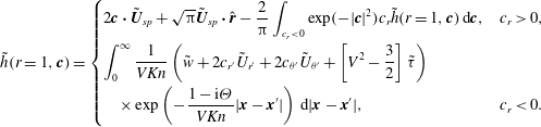 $$\begin{eqnarray}\tilde{h}(r=1,\boldsymbol{c})=\left\{\begin{array}{@{}ll@{}}\displaystyle 2\boldsymbol{c}\boldsymbol{\cdot }\tilde{\boldsymbol{U}}_{sp}+\sqrt{{\rm\pi}}\tilde{\boldsymbol{U}}_{sp}\boldsymbol{\cdot }\hat{\boldsymbol{r}}-\frac{2}{{\rm\pi}}\int _{c_{r}<0}\exp (-|\boldsymbol{c}|^{2})c_{r}\tilde{h}(r=1,\boldsymbol{c})\,\text{d}\boldsymbol{c},\quad & c_{r}>0,\\ \displaystyle \int _{0}^{\infty }\frac{1}{VKn}\left(\tilde{w}+2c_{r^{\prime }}\tilde{U} _{r^{\prime }}+2c_{{\it\theta}^{\prime }}\tilde{U} _{{\it\theta}^{\prime }}+\left[V^{2}-\frac{3}{2}\right]\tilde{{\it\tau}}\right)\quad \\ \displaystyle \quad \times \exp \left(-\frac{1-\text{i}{\it\Theta}}{VKn}|\boldsymbol{x}-\boldsymbol{x}^{\prime }|\right)\,\text{d}|\boldsymbol{x}-\boldsymbol{x}^{\prime }|,\quad & c_{r}<0.\end{array}\right.\end{eqnarray}$$
Equations (2.22)–(2.24) can be easily manipulated to yield a simplified expression for the scaled force on the sphere,
 $$\begin{eqnarray}\displaystyle \tilde{F} & = & \displaystyle \frac{2\sqrt{{\rm\pi}}}{3}\int _{1}^{\infty }\frac{1}{Kn}\sqrt{{\rm\pi}}r^{\prime 2}\left[W_{1}(r^{\prime })q_{1}(r^{\prime })-2W_{2}(r^{\prime })q_{2}(r^{\prime })\vphantom{\frac{3}{2}W_{4}(r^{\prime })}\right.\nonumber\\ \displaystyle & & \displaystyle \left.-\,4W_{3}(r^{\prime })q_{3}(r^{\prime })+\frac{3}{2}W_{4}(r^{\prime })\right]\,\text{d}r^{\prime }+\frac{{\rm\pi}}{3}\left(g+\frac{8}{\sqrt{{\rm\pi}}}\right),\end{eqnarray}$$
where the functions
 $W_{i}$
for
 $i=\{1,2,3,4\}$
are given in appendix B and the constant
 $g$
is given in (A 15).
3 Asymptotic limits
3.1 Unsteady flow
Analytical solutions are now presented in the continuum, slip and free-molecular asymptotic limits for unsteady flow. These are used in § 5 to provide benchmark results for the numerical solution outlined in § 4.
3.1.1 Continuum flow
 $(Kn\rightarrow 0~\mathit{and}~{\it\Theta}\rightarrow 0)$

In the continuum limit, the linearised Navier–Stokes equations, together with the no-slip boundary conditions, yield the radial and angular components of the bulk velocity (Landau & Lifshitz Reference Landau and Lifshitz1987):
 $$\begin{eqnarray}\displaystyle & \displaystyle \tilde{U} _{r}(r,{\it\theta})=\left\{\frac{2\hat{A}}{r^{3}}+2\hat{B}\exp (\text{i}\sqrt{2\text{i}{\it\beta}}r)\left(\frac{1}{r^{2}}-\frac{1}{\text{i}\sqrt{2\text{i}{\it\beta}}r^{3}}\right)\right\}\cos {\it\theta}, & \displaystyle\end{eqnarray}$$
 $$\begin{eqnarray}\displaystyle & \displaystyle \tilde{U} _{{\it\theta}}(r,{\it\theta})=\left\{\frac{\hat{A}}{r^{3}}-\hat{B}\exp (\text{i}\sqrt{2\text{i}{\it\beta}}r)\left(\frac{1}{\text{i}\sqrt{2\text{i}{\it\beta}}r^{3}}+\frac{\text{i}\sqrt{2\text{i}{\it\beta}}}{r}-\frac{1}{r^{2}}\right)\right\}\sin {\it\theta}, & \displaystyle\end{eqnarray}$$
 $$\begin{eqnarray}\displaystyle & \displaystyle \hat{A}=\frac{1}{2}\left(1-\frac{3}{\text{i}\sqrt{2\text{i}{\it\beta}}}-\frac{3}{2\text{i}{\it\beta}}\right), & \displaystyle\end{eqnarray}$$
 $$\begin{eqnarray}\displaystyle & \displaystyle \hat{B}=\frac{3\exp (-\text{i}\sqrt{2\text{i}{\it\beta}})}{2\text{i}\sqrt{2\text{i}{\it\beta}}} & \displaystyle\end{eqnarray}$$
 ${\it\Theta}=Kn^{2}{\it\beta}$
. The corresponding (continuum) force on the sphere is
 $$\begin{eqnarray}\tilde{F}_{con}={\rm\pi}Kn\left(3-3\text{i}\sqrt{2\text{i}{\it\beta}}-\frac{2\text{i}{\it\beta}}{3}\right),\end{eqnarray}$$
which has been scaled by
 $2a^{2}P/c_{m}$
. An identical force scale is used in all calculations.
3.1.2 Slip flow
$(Kn\ll 1~\mathit{and}~{\it\Theta}\ll 1)$

It has been shown (Cercignani Reference Cercignani2000; Sone Reference Sone2002; Ivchenko, Loyalka & Tompson Reference Ivchenko, Loyalka and Tompson2007) that the leading-order effect of gas rarefaction is formally obtained by solving the linearised Navier–Stokes equation subject to a slip boundary condition. This yields the required results for the bulk velocity:
 $$\begin{eqnarray}\displaystyle & \displaystyle \tilde{U} _{r}(r,{\it\theta})=\left\{\frac{2\hat{A}}{r^{3}}+2\hat{B}\exp \left(\text{i}\sqrt{2\text{i}{\it\beta}}r\right)\left(\frac{1}{r^{2}}-\frac{1}{\text{i}\sqrt{2\text{i}{\it\beta}}r^{3}}\right)\right\}\cos {\it\theta}, & \displaystyle\end{eqnarray}$$
 $$\begin{eqnarray}\displaystyle & \displaystyle \tilde{U} _{{\it\theta}}(r,{\it\theta})=\left\{\frac{\hat{A}}{r^{3}}-\hat{B}\exp \left(\text{i}\sqrt{2\text{i}{\it\beta}}r\right)\left(\frac{1}{\text{i}\sqrt{2\text{i}{\it\beta}}r^{3}}+\frac{\text{i}\sqrt{2\text{i}{\it\beta}}}{r}-\frac{1}{r^{2}}\right)\right\}\sin {\it\theta}, & \displaystyle\end{eqnarray}$$
 $$\begin{eqnarray}\displaystyle & \displaystyle \hat{A}=\frac{1}{2}\left\{1-\frac{(3+6{\it\sigma}Kn)\left(1-\displaystyle \frac{1}{\text{i}\sqrt{2\text{i}{\it\beta}}}\right)}{\text{i}\sqrt{2\text{i}{\it\beta}}+{\it\sigma}Kn\left(3\text{i}\sqrt{2\text{i}{\it\beta}}+2\text{i}{\it\beta}\right)}\right\}, & \displaystyle\end{eqnarray}$$
 $$\begin{eqnarray}\displaystyle & \displaystyle \hat{B}=\frac{3}{2}\left\{\frac{1+2{\it\sigma}Kn}{\text{i}\sqrt{2\text{i}{\it\beta}}+{\it\sigma}Kn\left(3\text{i}\sqrt{2\text{i}{\it\beta}}+2\text{i}{\it\beta}\right)}\right\}\exp \left(-\text{i}\sqrt{2\text{i}{\it\beta}}\right) & \displaystyle\end{eqnarray}$$
 ${\it\sigma}=1.016191\ldots$
. The corresponding scaled force is
 $$\begin{eqnarray}\displaystyle \displaystyle \tilde{F}_{slip} & \hspace{-2.0pt}=\hspace{-2.0pt} & \displaystyle \displaystyle -\frac{1}{3}{\rm\pi}Kn\nonumber\\ \displaystyle & & \displaystyle \displaystyle \times \,\left(\frac{4\text{i}{\it\beta}^{2}Kn\,{\it\sigma}-9\sqrt{2\text{i}{\it\beta}}(1+2{\it\sigma}Kn)+2\text{i}{\it\beta}(9\text{i}+\sqrt{2\text{i}{\it\beta}}+3[6\text{i}+\sqrt{2\text{i}{\it\beta}}]Kn{\it\sigma})}{\sqrt{2\text{i}{\it\beta}}+(3\sqrt{2\text{i}{\it\beta}}+2{\it\beta})Kn\,{\it\sigma}}\right).\nonumber\\ \displaystyle & & \displaystyle\end{eqnarray}$$
There is no temperature jump present at
 $O(Kn)$
and hence no temperature variation in the gas for slip flow (Takata et al.
Reference Takata, Sone and Aoki1993). For
 ${\it\beta}\gg 1$
, the flow is highly unsteady and vorticity is confined to a thin layer near the sphere surface; the thickness of this layer is
 $O({\it\delta})$
, where
 ${\it\delta}\ll a$
and
 ${\it\delta}=\sqrt{2{\it\mu}/({\it\rho}_{0}{\it\omega})}$
. In the opposite limit,
 ${\it\beta}\ll 1$
, we recover the steady solution, which is discussed in § 3.2.
3.1.3 Free-molecular flow
$(Kn\gg 1~\mathit{and/or}~{\it\Theta}\gg 1)$

If either
 $Kn\gg 1$
or
 ${\it\Theta}\gg 1$
is satisfied (or both are), then the flow is free-molecular. In the free-molecular limit, the linearised Boltzmann equation in (2.7) becomes
 $$\begin{eqnarray}\frac{1-\text{i}{\it\Theta}}{Kn}\tilde{h}+\boldsymbol{c}\boldsymbol{\cdot }\frac{\partial \tilde{h}}{\partial \boldsymbol{x}}=0.\end{eqnarray}$$
Equation (3.7) is solved by integrating along its characteristics (discussed above) and using the boundary conditions in (2.12). This gives
 $$\begin{eqnarray}\tilde{h}(\boldsymbol{x},\boldsymbol{c})=\left\{\begin{array}{@{}ll@{}}\displaystyle \tilde{h}_{0}\exp \left(\text{i}\frac{1-\text{i}{\it\Theta}}{Kn}\left|\boldsymbol{x}-\boldsymbol{x}_{0}\right|\right),\quad & \boldsymbol{c}\in R1,\\ 0,\quad & \boldsymbol{c}\in R2,\end{array}\right.\end{eqnarray}$$
where
 $$\begin{eqnarray}\tilde{h}_{0}(\boldsymbol{x}_{0},\boldsymbol{c})=2\boldsymbol{c}\boldsymbol{\cdot }\tilde{\boldsymbol{U}}_{sp}+\sqrt{{\rm\pi}}\tilde{\boldsymbol{U}}_{sp}\boldsymbol{\cdot }\hat{\boldsymbol{r}},\end{eqnarray}$$
and the regions
 $R1$
and
 $R2$
are defined in (2.14). As before,
 $(V,{\it\chi},{\it\psi})$
are the spherical coordinates of the particle velocity
 $\boldsymbol{c}$
; see (2.9) and (2.14). The density, bulk velocity and temperature are obtained by substituting (3.8) into (2.16), giving
 $$\begin{eqnarray}\displaystyle & \displaystyle \tilde{w}(r,{\it\theta})=\left[\bar{W}_{1}(r)+\sqrt{{\rm\pi}}\bar{R}_{1}(r)\right]\cos {\it\theta}, & \displaystyle\end{eqnarray}$$
 $$\begin{eqnarray}\displaystyle & \displaystyle \tilde{U} _{r}(r,{\it\theta})=\left[\bar{W}_{2}(r)+\sqrt{{\rm\pi}}\bar{R}_{2}(r)\right]\cos {\it\theta}, & \displaystyle\end{eqnarray}$$
 $$\begin{eqnarray}\displaystyle & \displaystyle \tilde{U} _{{\it\theta}}(r,{\it\theta})=\left[\bar{W}_{3}(r)+\sqrt{{\rm\pi}}\bar{R}_{3}(r)\right]\sin {\it\theta}, & \displaystyle\end{eqnarray}$$
 $$\begin{eqnarray}\displaystyle & \displaystyle \tilde{{\it\tau}}(r,{\it\theta})=\left[\bar{W}_{4}(r)+\sqrt{{\rm\pi}}\bar{R}_{4}(r)\right]\cos {\it\theta}, & \displaystyle\end{eqnarray}$$
 $\bar{W}_{i}(r),\bar{R}_{i}(r)$
for
 $i\in \{1,2,3,4\}$
are defined in appendix C. The scaled force is obtained from (2.22) and (2.23):
 $$\begin{eqnarray}\tilde{F}_{fm}=\frac{\sqrt{{\rm\pi}}}{3}\left({\rm\pi}+8\right).\end{eqnarray}$$
For
 ${\it\Theta}\gg Kn$
, the flow is confined to a thin boundary layer of thickness
 $O(c_{m}/{\it\omega})$
, i.e. the average distance a gas particle travels in one oscillation cycle. When
 $Kn\ll {\it\Theta}$
, the unsteady term in (3.7) vanishes and steady flow is recovered; see § 3.2.
3.2 Steady flow
$({\it\Theta}=0)$

The corresponding results are now summarised for steady flow. These are obtained from the results in the preceding section by taking the limit
 ${\it\Theta}\rightarrow 0$
, and are used to validate the numerical solution specified in § 4. The steady flow asymptotic solutions have been reported previously and are provided here for completeness.
3.2.1 Continuum flow
$(Kn\rightarrow 0)$

The bulk velocity in the gas is
 $$\begin{eqnarray}\displaystyle U_{r}(r,{\it\theta})=\left(\frac{3}{2r}-\frac{1}{2r^{3}}\right)\cos {\it\theta},\quad \displaystyle U_{{\it\theta}}(r,{\it\theta})=-\left(\frac{3}{4r}+\frac{1}{4r^{3}}\right)\sin {\it\theta},\end{eqnarray}$$
and the corresponding scaled force is
 $$\begin{eqnarray}F_{con}=3{\rm\pi}Kn.\end{eqnarray}$$
3.2.2 Slip flow
$(Kn\ll 1)$

The slip solution for steady flow is obtained by taking the same limit,
 ${\it\Theta}\rightarrow 0$
, in (3.4) while keeping
 $Kn$
finite. This gives the following result for the bulk velocity (Takata et al.
Reference Takata, Sone and Aoki1993):
 $$\begin{eqnarray}\displaystyle & \displaystyle U_{r}(r,{\it\theta})=\left\{\frac{3}{2}\left(\frac{1+2{\it\sigma}Kn}{1+3{\it\sigma}Kn}\right)\frac{1}{r}-\frac{1}{2}\left(\frac{1}{1+3{\it\sigma}Kn}\right)\frac{1}{r^{3}}\right\}\cos {\it\theta}, & \displaystyle\end{eqnarray}$$
 $$\begin{eqnarray}\displaystyle & \displaystyle U_{{\it\theta}}(r,{\it\theta})=-\!\left\{\frac{3}{4}\left(\frac{1+2{\it\sigma}Kn}{1+3{\it\sigma}Kn}\right)\frac{1}{r}+\frac{1}{4}\left(\frac{1}{1+3{\it\sigma}Kn}\right)\frac{1}{r^{3}}\right\}\sin {\it\theta}, & \displaystyle\end{eqnarray}$$
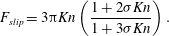 $$\begin{eqnarray}F_{slip}=3{\rm\pi}Kn\left(\frac{1+2{\it\sigma}Kn}{1+3{\it\sigma}Kn}\right).\end{eqnarray}$$
Equation (3.15) coincides with the result of Ivchenko et al. (Reference Ivchenko, Loyalka and Tompson2007).
3.2.3 Free-molecular flow
$(Kn\gg 1)$

The density, bulk velocity and temperature are (Takata et al. Reference Takata, Sone and Aoki1993)
 $$\begin{eqnarray}\displaystyle & \displaystyle w=\displaystyle \frac{\sqrt{{\rm\pi}}}{6}\left\{\left(1+\frac{6}{{\rm\pi}}\right)\frac{1}{r^{2}}-(r^{2}-1)^{1/2}\left(2+\frac{1}{r^{2}}\right)+2r\right\}\cos {\it\theta}, & \displaystyle\end{eqnarray}$$
 $$\begin{eqnarray}\displaystyle & \displaystyle U_{r}=\displaystyle \left\{-\frac{1}{2}-\frac{1}{2}\left(1-\frac{1}{r^{2}}\right)^{3/2}+\frac{1}{4r^{3}}+\frac{1}{8}\left[1+\frac{1}{r^{2}}+\frac{(r^{2}-1)^{2}}{2r^{3}}\log \left(\frac{r-1}{r+1}\right)\right]\right\}\cos {\it\theta}, & \displaystyle \nonumber\\ \displaystyle & & \displaystyle\end{eqnarray}$$
 $$\begin{eqnarray}\displaystyle \hspace{-15.00002pt} & \displaystyle U_{{\it\theta}}=\displaystyle \left\{\frac{1}{2}+\frac{1}{8r^{3}}+\frac{1}{4}\left(1-\frac{1}{r^{2}}\right)^{1/2}\left(2+\frac{1}{r^{2}}\right)\right. & \displaystyle \nonumber\\ \displaystyle \hspace{-15.00002pt} & \qquad \qquad \qquad \qquad \displaystyle \left.\vphantom{\left(2+\frac{1}{r^{2}}\right)^{1/2}}-\frac{1}{32}\left[6-\frac{2}{r^{2}}+\frac{3r^{4}-2r^{2}-1}{r^{3}}\log \left(\frac{r-1}{r+1}\right)\right]\right\}\sin {\it\theta}, & \displaystyle\end{eqnarray}$$
 $$\begin{eqnarray}\displaystyle & \displaystyle {\it\tau}=\displaystyle -\frac{\cos {\it\theta}}{3\sqrt{{\rm\pi}}r^{2}}. & \displaystyle\end{eqnarray}$$
At any instant in time in an unsteady flow, the distribution function for outgoing particle velocities is a Maxwellian with a mean velocity
 $U_{mean}\,\hat{\boldsymbol{z}}$
, where
 $U_{mean}\in [-U_{0},U_{0}]$
. Since particles do not collide in the free-molecular limit, the distribution function of outgoing particle velocities is identical to that generated by a sphere moving with constant velocity
 $U_{mean}\,\hat{\boldsymbol{z}}$
. The steady and unsteady free-molecular forces are therefore identical, and given by (3.11).
4 Numerical methods
Numerical methods to solve (2.21) are detailed in this section. Distinct methods for steady and unsteady flows are discussed in §§ 4.1 and 4.2 respectively, because the asymptotic behaviour of these flows far from the sphere is different.
4.1 Steady flow
To solve (2.21) for steady flow, the region of integration is first truncated at a radius
 $r=R_{N}\gg 1$
, giving
 $$\begin{eqnarray}q_{k}(r)=\int _{1}^{R_{N}}\mathop{\sum }_{m=1}^{4}K_{km}(r,r^{\prime })q_{m}(r^{\prime })\,\text{d}r^{\prime }+T_{k}(r),\end{eqnarray}$$
where
 $k\in \{1,2,3,4\}$
is implied throughout. Asymptotic solutions for small
 $Kn$
in § 3.2 show that the bulk velocity asymptotically decays
 ${\sim}r^{-1}$
far from the sphere;
 $R_{N}$
must therefore be very large for a negligible truncation error (Takata et al.
Reference Takata, Sone and Aoki1993). To reduce the computational domain, and hence computational time, the approach proposed by Takata et al. (Reference Takata, Sone and Aoki1993) is used. Because the flow must be near-continuum far from the sphere, asymptotic solutions for small
 $Kn$
are used in this region in place of the unknown functions
 $q_{k}$
in (4.1). We therefore choose some radius
 $R_{M}\in (1,R_{N})$
, beyond which the small-Kn asymptotic solution applies. Thus, (4.1) becomes
 $$\begin{eqnarray}q_{k}(r)=\int _{1}^{R_{M}}\mathop{\sum }_{m=1}^{4}K_{km}(r,r^{\prime })q_{m}(r^{\prime })\,\text{d}r^{\prime }+\int _{R_{M}}^{R_{N}}\mathop{\sum }_{m=1}^{4}K_{km}(r,r^{\prime })Q_{m}(r^{\prime })\,\text{d}r^{\prime }+T_{k}(r),\end{eqnarray}$$
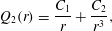
where the near-continuum solutions
 $Q_{m}(r)$
have the general form (Takata et al.
Reference Takata, Sone and Aoki1993)
 $$\begin{eqnarray}\displaystyle \displaystyle Q_{1}(r) & \hspace{-2.0pt}=\hspace{-2.0pt} & \displaystyle \displaystyle \frac{C_{1}Kn-C_{3}}{r^{2}},\end{eqnarray}$$
 $$\begin{eqnarray}\displaystyle \displaystyle Q_{2}(r) & \hspace{-2.0pt}=\hspace{-2.0pt} & \displaystyle \displaystyle \frac{C_{1}}{r}+\frac{C_{2}}{r^{3}},\end{eqnarray}$$
 $$\begin{eqnarray}\displaystyle \displaystyle Q_{3}(r) & \hspace{-2.0pt}=\hspace{-2.0pt} & \displaystyle \displaystyle -\frac{C_{1}}{2r}+\frac{C_{2}}{2r^{3}},\end{eqnarray}$$
 $$\begin{eqnarray}\displaystyle \displaystyle Q_{4}(r) & \hspace{-2.0pt}=\hspace{-2.0pt} & \displaystyle \displaystyle \frac{C_{3}}{r^{2}}.\end{eqnarray}$$
 $C_{1},C_{2}$
and
 $C_{3}$
are coefficients to be evaluated by matching
 $Q_{m}(r)$
to numerical solutions at
 $r=R_{M}$
; see below.
Next, we apply the singularity subtraction technique (Loyalka & Tompson Reference Loyalka and Tompson2009) to the first integral on the right-hand side of (4.2). This removes the singularity at
 $r=r^{\prime }$
in the kernel
 $K_{km}(r,r^{\prime })$
and improves convergence. Equation (4.2) yields
 $$\begin{eqnarray}\displaystyle \displaystyle \mathop{\sum }_{m=1}^{4}A_{km}(r)q_{k}(r) & \hspace{-2.0pt}=\hspace{-2.0pt} & \displaystyle \displaystyle \int _{1}^{R_{M}}\mathop{\sum }_{m=1}^{4}K_{km}(r,r^{\prime })\left(q_{m}(r^{\prime })-q_{m}(r)\right)\text{d}r^{\prime }\nonumber\\ \displaystyle & & \displaystyle \displaystyle +\int _{R_{M}}^{R_{N}}\mathop{\sum }_{m=1}^{4}K_{km}(r,r^{\prime })Q_{m}(r^{\prime })\,\text{d}r^{\prime }+T_{k}(r),\end{eqnarray}$$
where
 $$\begin{eqnarray}A_{km}(r)={\it\delta}_{km}-\int _{1}^{R_{M}}K_{km}(r,r^{\prime })\,\text{d}r^{\prime }\end{eqnarray}$$
and
 ${\it\delta}_{km}$
is the Kronecker delta function.
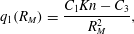
The coefficients
 $C_{1},C_{2},C_{3}$
in (4.3) are calculated by matching (4.3) to numerical solutions of the integral equations, (4.4), at
 $r=R_{M}$
, i.e.
 $$\begin{eqnarray}\displaystyle \displaystyle q_{1}(R_{M}) & \hspace{-2.0pt}=\hspace{-2.0pt} & \displaystyle \displaystyle \frac{C_{1}Kn-C_{3}}{R_{M}^{2}},\end{eqnarray}$$
 $$\begin{eqnarray}\displaystyle \displaystyle q_{2}(R_{M}) & \hspace{-2.0pt}=\hspace{-2.0pt} & \displaystyle \displaystyle \frac{C_{1}}{R_{M}}+\frac{C_{2}}{R_{M}^{3}},\end{eqnarray}$$
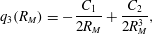 $$\begin{eqnarray}\displaystyle \displaystyle q_{3}(R_{M}) & \hspace{-2.0pt}=\hspace{-2.0pt} & \displaystyle \displaystyle -\frac{C_{1}}{2R_{M}}+\frac{C_{2}}{2R_{M}^{3}},\end{eqnarray}$$
 $q_{1}(R_{M}),q_{2}(R_{M}),q_{3}(R_{M})$
are found by solving (4.4). Equations (4.4) and (4.6) thus form a closed set of equations.
Equation (4.4) is solved by first dividing the domain
 $r\in [1,R_{M}]$
into two subdomains,
 $[1,R_{L}]$
and
 $[R_{L},R_{M}]$
, where
 $R_{L}=Kn+1$
. The subdomain
 $[1,R_{L}]$
is further divided into
 $L_{1}$
intervals, and the resulting integral in each interval is evaluated using Gauss–Legendre (GL) quadrature of order
 $N_{1}$
. The second subdomain
 $[R_{L},R_{M}]$
is divided into
 $L_{2}$
intervals where the integral in each interval is evaluated with GL quadrature of order
 $N_{2}$
. This allows a dense mesh to be used close to the sphere where large velocity gradients are expected. Additionally, the integral with limits
 $[R_{M},R_{N}]$
is evaluated using GL quadrature of order
 $N_{c}$
. A schematic of the integration domain is shown in figure 4.
Schematic illustrating division of the integration domain into three subdomains. The subdomain
 $[1,R_{L}]$
is divided into
 $L_{1}$
intervals, each of which is subdivided into
 $N_{1}$
subintervals. The subdomain
 $[R_{L},R_{M}]$
is divided into
 $L_{2}$
intervals, each of which is subdivided into
 $N_{2}$
subintervals. The subdomain
 $[R_{M},R_{N}]$
is divided into
 $N_{c}$
intervals.

This produces the following system of linear equations:
 $$\begin{eqnarray}\displaystyle \displaystyle \mathop{\sum }_{m=1}^{4}A_{km}(r_{i})q_{k}(r_{i}) & \hspace{-2.0pt}=\hspace{-2.0pt} & \displaystyle \displaystyle \mathop{\sum }_{j=1}^{N_{L}}w_{j}\left\{\mathop{\sum }_{m=1}^{4}K_{km}(r_{i},r_{j})(q_{m}(r_{j})-q_{m}(r_{i}))\right\}\nonumber\\ \displaystyle & & \displaystyle +\,\displaystyle \mathop{\sum }_{p=1}^{N_{c}}w_{p}\frac{R_{N}-R_{M}}{2}\mathop{\sum }_{m=1}^{4}K_{km}(r_{i},r_{p})Q_{m}(r_{p})+T_{k}(r_{i})\end{eqnarray}$$
and
 $$\begin{eqnarray}\displaystyle \displaystyle \mathop{\sum }_{m=1}^{4}A_{km}(R_{M})q_{k}(R_{M}) & \hspace{-2.0pt}=\hspace{-2.0pt} & \displaystyle \displaystyle \mathop{\sum }_{j=1}^{N_{L}}w_{j}\left\{\mathop{\sum }_{m=1}^{4}K_{km}(R_{M},r_{j})\left(q_{m}(r_{j})-q_{m}(R_{M})\right)\right\}\nonumber\\ \displaystyle & & \displaystyle +\,\displaystyle \mathop{\sum }_{p=1}^{N_{c}}w_{p}\frac{R_{N}-R_{M}}{2}\mathop{\sum }_{m=1}^{4}K_{km}(R_{M},r_{p})Q_{m}(r_{p})+T_{k}(R_{M}),\end{eqnarray}$$
where
 $$\begin{eqnarray}N_{L}=N_{1}L_{1}+N_{2}L_{2}\end{eqnarray}$$
is the total number of meshpoints. The
 $j$
th discretised node to the right of
 $r=1$
in figure 4 is
 $$\begin{eqnarray}r_{j}=\left\{\begin{array}{@{}ll@{}}\displaystyle \frac{R_{L}-1}{2L_{1}}y_{1+(j-1)\,\text{mod}\,N_{1}}+\left(2\left\lfloor \frac{j-1}{N_{1}}\right\rfloor +1\right)\frac{R_{L}-1}{2L_{1}}+1,\quad & j=1,\ldots ,N_{1}L_{1},\\ \displaystyle \frac{R_{M}-R_{L}}{2L_{2}}z_{1+(j-N_{1}L_{1}-1)\,\text{mod}\,N_{2}}\quad \\ \quad \displaystyle +\left(2\left\lfloor \frac{j-N_{1}L_{1}-1}{N_{2}}\right\rfloor +1\right)\frac{R_{M}-R_{L}}{2L_{2}}+R_{L},\quad & j=N_{1}L_{1}+1,\ldots ,N_{L},\end{array}\right.\end{eqnarray}$$
where
 $r_{i},r_{j}\in (1,R_{M})$
and the corresponding weights are
 $$\begin{eqnarray}w_{j}=\left\{\begin{array}{@{}ll@{}}\displaystyle u_{1+(j-1)\,\text{mod}\,N_{1}}\frac{R_{L}-1}{2L_{1}},\quad & j=1,\ldots ,N_{1}L_{1},\\ \displaystyle v_{1+(j-N_{1}L_{1}-1)\,\text{mod}\,N_{2}}\frac{R_{M}-R_{L}}{2L_{2}},\quad & j=N_{1}L_{1}+1,\ldots ,N_{L}.\end{array}\right.\end{eqnarray}$$
Here,
 $y_{{\it\alpha}}$
and
 $u_{{\it\alpha}}$
are the usual GL abscissas and weights with
 $y_{{\it\alpha}}\in (-1,1)$
for
 ${\it\alpha}=1,2,\ldots ,N_{1}$
. Similarly,
 $z_{{\it\beta}}$
and
 $v_{{\it\beta}}$
are GL abscissas and weights of order
 $N_{2}$
for
 ${\it\beta}=1,2,\ldots ,N_{2}$
(note that
 ${\it\beta}$
here refers to an index, not the inverse Stokes number). The
 $p$
th discretised node to the right of
 $R_{M}$
in figure 4 is
 $$\begin{eqnarray}r_{p}=\frac{R_{N}-R_{M}}{2}b_{p}+\frac{R_{M}+R_{N}}{2},\quad p=1,\ldots ,N_{c},\end{eqnarray}$$
where
 $r_{p}\in (R_{M},R_{N})$
and
 $b_{p}$
are the usual GL abscissas with corresponding weights
 $w_{p}$
.
Equations (4.6)–(4.8) specify a fully determined linear system of equations that can be solved numerically. This system is implemented and solved in Mathematica, the results of which are given in § 5.2; see § 4.3 for details of the numerical implementation.
4.2 Unsteady flow
The asymptotic solution for unsteady flow in the continuum limit (i.e. for infinitesimal
 $Kn$
) shows that the bulk velocity decays far from the sphere as
 ${\sim}r^{-2}$
, which is faster than the rate for the steady case; cf. (3.1) and (3.12a,b
). This negates the utility of the asymptotic solution far from the sphere; we therefore choose the truncation radius
 $R_{N}=R_{M}$
; see figure 4. Proceeding with the singularity subtraction method (Loyalka & Tompson Reference Loyalka and Tompson2009), (2.21) then becomes
 $$\begin{eqnarray}\mathop{\sum }_{m=1}^{4}A_{km}(r)q_{k}(r)=\int _{1}^{R_{M}}\mathop{\sum }_{m=1}^{4}K_{km}(r,r^{\prime })\left(q_{m}(r^{\prime })-q_{m}(r)\right)\,\text{d}r^{\prime }+T_{k}(r),\end{eqnarray}$$
where all variables are as defined in the preceding section.
Similarly to the steady case, (4.13) is solved by first dividing the domain
 $r\in [1,R_{M}]$
into two subdomains,
 $[1,R_{L}]$
and
 $[R_{L},R_{M}]$
, where
 $R_{L}=1+\min (Kn,Kn/{\it\Theta})$
. This choice of
 $R_{L}$
ensures that all steep gradients in the transport variables near the surface can be captured accurately. The subdomains
 $[1,R_{L}]$
and
 $[R_{L},R_{M}]$
are discretised as before, leading to the following system:
 $$\begin{eqnarray}\mathop{\sum }_{m=1}^{4}A_{km}(r_{i})q_{k}(r_{i})=\mathop{\sum }_{j=1}^{N_{L}}w_{j}\left\{\mathop{\sum }_{m=1}^{4}K_{km}(r_{i},r_{j})\left(q_{m}(r_{j})-q_{m}(r_{i})\right)\right\}+T_{k}(r_{i}),\end{eqnarray}$$
where the abscissas
 $r_{i},r_{j}$
and corresponding weights
 $w_{j}$
are given in (4.9)–(4.11). The integration domain for the unsteady problem is therefore a subset of that for the steady case.
Details of the numerical implementation of the above equations for the steady and unsteady problems are discussed in the next section.
4.3 Numerical implementation
The kernel and inhomogeneous terms of the integral equations defined in appendix B are written in terms of Meijer-G functions, which are evaluated in Mathematica. Integration of the kernel functions is required after applying the singularity subtraction method, and this is performed numerically using Mathematica’s NIntegrate function with a working precision of at least
 $45$
significant figures. Greater working precision is required as
 $R_{M}$
is increased. Additionally, the precision of all other calculations is set to
 $100$
significant figures in Mathematica because this setting ensures the Meijer-G functions are evaluated to at least
 $45$
significant figures.
Numerical results are calculated for
 $Kn\in [0.1,10]$
and for unsteady flow
 ${\it\Theta}\in [0.1,10]$
. For each Knudsen number and frequency ratio, different values for the computational parameters
 $R_{L}$
,
 $R_{M}$
,
 $R_{N}$
,
 $L_{1}$
and
 $L_{2}$
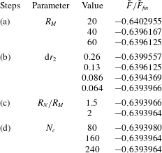
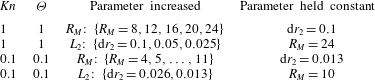
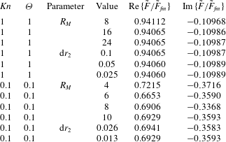
are used. These computational parameters are increased systematically to a point where they do not change the calculated force on the sphere. This numerical convergence procedure, used to obtain accurate solutions, is presented in appendix D.
5 Results and discussion
In the continuum limit, the linear gas flow driven by a solid sphere that is moving with constant velocity is isothermal (Stokes Reference Stokes1880). However, a temperature jump always exists at the surface of a sphere in a real flow due to the finite mean free path of the gas – this occurs at
 $O(Kn^{2})$
(Takata et al.
Reference Takata, Sone and Aoki1993). It is well established that this temperature jump is directly proportional to the gradient of the normal stress in the gas (Sone Reference Sone2002) and exists at all degrees of gas rarefaction, even for a linearised flow (small Mach number). As such, the linear flow driven by a sphere cannot be treated as isothermal.
This finding appears unintuitive but can be easily understood by considering the distribution function for a free-molecular gas flow generated by a sphere moving with constant velocity. For simplicity, we consider the complementary case where the sphere is held stationary with an impinging uniform and steady free-molecular flow (Takata et al. Reference Takata, Sone and Aoki1993). We give an overview of this analysis in § 5.1 as it provides a foundation for the numerical results at arbitrary Knudsen number.
5.1 Temperature jump in the free-molecular limit
Consider a stationary solid sphere in a uniform and steady gas flow in the free-molecular limit, i.e.
 $Kn\gg 1$
. Far from the sphere, the gas velocity is unidirectional in the Cartesian
 $z$
direction with constant magnitude
 $U_{0}$
, and the gas temperature
 $T_{\infty }$
is constant. Gas particles interact with the surface of the sphere via the diffuse boundary condition. The temperatures of the sphere and the free-stream gas are identical, as specified in § 2.
The mass distribution function of particles incoming to the sphere surface (
 $c_{r}<0$
) is a Maxwellian centred at a bulk velocity
 $\boldsymbol{U}_{\infty }=U_{0}\hat{\boldsymbol{z}}$
with temperature
 $T_{\infty }$
. In contrast, due to the diffuse boundary condition, the distribution function for particles leaving the sphere surface (
 $c_{r}>0$
) is a Maxwellian centred at a bulk velocity of zero, with the same temperature
 $T_{\infty }$
; these are the conditions at the surface of the sphere. The complete mass distribution function for molecular velocities in the radial direction,
 $c_{r}$
, at the sphere surface, i.e. the one-dimensional distribution, is therefore
 $$\begin{eqnarray}\displaystyle F_{1D}=\sqrt{\frac{m}{2{\rm\pi}kT_{\infty }}}\left\{\begin{array}{@{}ll@{}}\displaystyle \exp \left(-\frac{m}{2kT_{\infty }}c_{r}^{2}\right),\quad & c_{r}>0,\\ \displaystyle \exp \left(-\frac{m}{2kT_{\infty }}\left[c_{r}-\boldsymbol{U}_{\infty }\boldsymbol{\cdot }\hat{\boldsymbol{r}}\right]^{2}\right),\quad & c_{r}<0,\end{array}\right.\end{eqnarray}$$
where
 $\boldsymbol{U}_{\infty }=U_{0}\hat{\boldsymbol{z}}=U_{0}(\cos {\it\theta}\,\hat{\boldsymbol{r}}-\sin {\it\theta}\,\hat{{\bf\theta}})$
; see (2.2).
Consider the position
 $(r=a,{\it\theta}={\rm\pi})$
on the sphere surface; the gas impinges at normal incidence to the sphere at this position. The outward normal,
 $\hat{\boldsymbol{r}}$
, to the surface is therefore in the direction opposite to the uniform velocity
 $\boldsymbol{U}_{\infty }$
. In this case, the one-dimensional distribution function in (5.1) becomes
 $$\begin{eqnarray}\displaystyle F_{1D}=\sqrt{\frac{m}{2{\rm\pi}kT_{\infty }}}\left\{\begin{array}{@{}ll@{}}\displaystyle \exp \left(-\frac{m}{2kT_{\infty }}c_{r}^{2}\right),\quad & c_{r}>0,\\ \displaystyle \exp \left(-\frac{m}{2kT_{\infty }}\left[c_{r}+U_{0}\right]^{2}\right),\quad & c_{r}<0,\end{array}\right.\end{eqnarray}$$
which is illustrated in figure 5. It should be noted that this distribution function has a ‘width’ (or variance) that is larger than the original Maxwellian distribution of the gas far from the sphere. Because the gas temperature is directly proportional to the variance of the distribution of molecular velocities, this immediately establishes that the gas temperature at the surface of the sphere is higher than that of the free stream and solid surface. That is, the gas is hotter than the solid sphere at the position
 $(r=a,{\it\theta}={\rm\pi})$
.
The one-dimensional mass distribution function,
 $F_{1D}$
, at a position
 $(r=a,{\it\theta}={\rm\pi})$
on the surface of the stationary sphere in a uniform and steady free-molecular gas flow,
 $\boldsymbol{U}_{\infty }=U_{0}\hat{\boldsymbol{z}}$
. The distribution function is shown for incoming particles (
 $c_{r}<0$
, red) and outgoing particles (
 $c_{r}>0$
, blue). This distribution function has a larger variance than that of a Maxwellian at the equilibrium temperature, i.e. the gas temperature represented by this distribution is higher than equilibrium.

Identical arguments establish that the gas is cooler than
 $T_{\infty }$
at
 $(r=a,{\it\theta}=0)$
and its temperature is equal to that of the sphere at
 $(r=a,{\it\theta}={\rm\pi}/2)$
. This shows that the gas temperature around the sphere surface varies and is different from that of the sphere. Consequently, there is a temperature jump in the gas at the surface which results in a non-zero temperature variation around the sphere, i.e. the flow is non-isothermal. This phenomenon is frequently referred to as thermal polarisation, and always occurs if a section of the solid surface is oriented normal to the flow direction. It exists at all Knudsen numbers to varying degrees, vanishing in the continuum limit. Interestingly, the sign of the thermal polarisation for small Knudsen number is opposite to that of the free-molecular flow (Aoki & Sone Reference Aoki and Sone1987), i.e. the temperature of the gas is lower than that of the solid sphere at the position
 $(r=a,{\it\theta}={\rm\pi})$
and higher at (
 $r=a$
,
 ${\it\theta}={\rm\pi}/2$
).
Steady flow: numerical results for the radial dependence of the density
 $q_{1}(r)$
, velocities
 $q_{2}(r)$
,
 $q_{3}(r)$
and temperature
 $q_{4}(r)$
as a function of the radius
 $r$
, using the present method. Results are given for
 $Kn=0.1$
(red solid),
 $Kn=1$
(green dashed) and
 $Kn=10$
(black dotted). The solutions for
 $Kn=10$
are shown as solid circles, with the dotted line being the interpolated curve; the observed spacing of these points is due to the use of low-order quadrature. The dependences of the macroscopic variables on the polar angle
 ${\it\theta}$
are given in (2.17).

5.2 Validation for steady flow
We now return to the original problem of a sphere moving in a quiescent gas at finite Knudsen number. Before presenting the new results for unsteady flow, we validate the numerical method by comparing our calculations for steady flow with published literature results. This also provides benchmark data to investigate the effects of unsteadiness on the flow field and drag force. Due to axisymmetry, results are presented only for the radial dependences of the density, velocity and temperature field; the polar angle dependences are given in (2.17).
Figure 6 shows these radially dependent terms, i.e.
 $q_{1},q_{2},q_{3},q_{4}$
, for the near-continuum (
 $Kn=0.1$
), transition (
 $Kn=1$
) and near-collisionless (
 $Kn=10$
) flow regimes. As expected, the tangential component of the slip velocity,
 $q_{slip}=q_{3}(1)+1$
, increases with increasing Kn; note that
 $q_{3}(1)=-1$
coincides with the no-slip condition. The density and temperature fields are similar to their equilibrium solutions (i.e. no density or temperature variations) for near-continuum flow; see figures 6(a,d). Finite and increasing Knudsen number enhances the density and temperature variations, in line with the discussion of the previous section. Most importantly, flow at finite Knudsen number is non-isothermal and compressible.
Figure 7 presents a comparison of the numerical results (for finite Knudsen number,
 $Kn$
) with the asymptotic solutions of § 3 for the bulk velocity; results are given in the appropriate near-continuum and near-collisionless regimes, with
 $Kn=0.1$
and
 $10$
. Strikingly, the numerical results for both
 $Kn=0.1$
and
 $10$
are in excellent agreement with the slip solution of (3.14) and the free-molecular solution of (3.16) respectively. While slight differences are clearly observable, this is expected because the analytical solutions in (3.14) and (3.16) are strictly valid in the asymptotic limits
 $Kn\rightarrow 0$
and
 $Kn\rightarrow \infty$
respectively. This provides a second validation of the numerical method.
Steady flow: comparison of current numerical results with asymptotic solutions for (a)
 $Kn=0.1$
and (b)
 $Kn=10$
. Solid lines: current numerical results. Dashed lines: asymptotic slip and free-molecular (FM) solutions, (3.14) and (3.16) respectively. The black (upper) and red (lower) lines are the radial dependences of the radial velocity,
 $q_{2}(r)$
, and angular velocity,
 $q_{3}(r)$
, respectively. The numerical solutions for (b) are solid circles with interpolated (solid line) curves. The dependence of the bulk velocity on the polar angle
 ${\it\theta}$
is given in (2.17).

Figure 8 compares the density, bulk velocity and temperature profiles obtained using the current numerical method with the results of Law & Loyalka (Reference Law and Loyalka1986) (for non-isothermal flows). Again, excellent agreement is found for the distinct cases
 $Kn=1$
and
 $10$
. It should be noted that the data in Law & Loyalka (Reference Law and Loyalka1986) appear to contain some typographical errors, which have been excluded from all comparisons in this article.
Next, we compare our results with both the non-isothermal and isothermal results of Law & Loyalka (Reference Law and Loyalka1986), which were reported for
 $Kn=0.1$
. Law & Loyalka (Reference Law and Loyalka1986) obtained isothermal results by ignoring the temperature equation; that is, by setting
 $q_{4}=0$
in the above formulation. As discussed above, the steady flow around a sphere is strictly non-isothermal, and this comparison is presented only to highlight the effect of imposing an (artificial) isothermal assumption. Figure 9 gives a comparison of these literature data with the results of the present numerical method.
Steady flow: comparison of current numerical results and the non-isothermal data of Law & Loyalka (Reference Law and Loyalka1986) for (a)
 $Kn=1$
and (b)
 $Kn=10$
. Solid lines: current numerical results. Points: Law & Loyalka (Reference Law and Loyalka1986). Radial dependences of the density
 $q_{1}(r)$
, radial velocity
 $q_{2}(r)$
, angular velocity
 $q_{3}(r)$
and temperature
 $q_{4}(r)$
are given. The current numerical results are obtained by interpolating the numerical solutions at GL abscissas. See (2.17) for the dependences of the macroscopic variables on the polar angle
 ${\it\theta}$
.

Steady flow for
 $Kn=0.1$
: comparison of current numerical results for the radial dependences of the macroscopic variables and the data of Law & Loyalka (Reference Law and Loyalka1986). (a) Solid lines: current numerical results for the radial velocity
 $q_{2}(r)$
and angular velocity
 $q_{3}(r)$
. Points: Law & Loyalka (Reference Law and Loyalka1986) non-isothermal radial and angular velocity. (b) Solid lines: current numerical results for the density
 $q_{1}(r)$
and temperature
 $q_{4}(r)$
. Points: Law & Loyalka (Reference Law and Loyalka1986) non-isothermal density (squares) and temperature (diamonds). Dotted line: Law & Loyalka (Reference Law and Loyalka1986) isothermal density.

Excellent agreement between the non-isothermal results of Law & Loyalka (Reference Law and Loyalka1986) and the present method is observed for the bulk velocity; see figure 9(a). However, figure 9(b) shows that the density and temperature numerical results of the current study are significantly different from the non-isothermal data of Law & Loyalka (Reference Law and Loyalka1986). The non-isothermal density and temperature solutions from Law & Loyalka (Reference Law and Loyalka1986) appear to increase with radius from the sphere – this is unexpected because the temperature field must approach the equilibrium result far from the sphere, i.e.
 $q_{4}(r)\rightarrow 0$
as
 $r\rightarrow \infty$
. Interestingly, we find good agreement between our non-isothermal density numerical solutions and the isothermal density results of Law & Loyalka (Reference Law and Loyalka1986); see figure 9(b). Compared with larger Knudsen numbers (where excellent agreement is observed, see figure 8), the numerical simulations of flows at small Knudsen numbers converge slower and require more computational time to obtain solutions of similar accuracy; this may explain these deviations.
In table 1, we present tabulated numerical data for the normalised force,
 $\tilde{F}/\tilde{F}_{fm}$
, where
 $\tilde{F}_{fm}$
is the free-molecular force (3.11), obtained using the present method over a comprehensive range of Knudsen numbers. Available data from the literature are also presented in table 1. We find reasonable agreement with the data of Law & Loyalka (Reference Law and Loyalka1986) and excellent agreement with the data of Takata et al. (Reference Takata, Sone and Aoki1993), both of which utilise a finite-differencing scheme under non-isothermal conditions. Our results also approach the correct asymptotic limits for both near-continuum and free-molecular flow.
The new high-accuracy data set for steady flow generated by a sphere, listed under ‘current results’ in table 1, is accurate to four decimal places. The linearised Boltzmann equation for hard spheres has been solved over a wide range of Knudsen numbers for this steady flow problem (Takata et al. Reference Takata, Sone and Aoki1993). Table 1 presents an equivalent range for the Boltzmann–BGK equation, which is larger than reported previously for this collision model. This data set is expected to be of value for the benchmarking and validation of computational and analytical studies.
The normalised force
 $\tilde{F}/\tilde{F}_{fm}$
(see (2.25) and (3.11)) obtained in the current study, and by Law & Loyalka (Reference Law and Loyalka1986) and Takata et al. (Reference Takata, Sone and Aoki1993), for a range of Knudsen numbers. The current results are accurate to four decimal places. Asymptotic results are included for the near-continuum (slip) (3.15) and free-molecular (FM) (3.11) regimes.

5.3 Unsteady flow
Next, we present results for unsteady flow over a broad range of Knudsen numbers,
 $Kn$
, and frequency ratios,
 ${\it\Theta}$
, encompassing the near-continuum to near-collisionless regimes. We first validate the numerical method for unsteady flow by comparing its solutions with the analytical asymptotic solutions presented in § 3.1.
Unsteady flow for
 $Kn=30,{\it\Theta}=100$
: comparison of current numerical solutions (solid line) and asymptotic free-molecular (FM) solutions in (3.10) (dotted line). The magnitude,
 $|q_{i}(r)|$
, and phase,
 ${\it\zeta}_{i}(r)$
, are given for (a,b) density,
 $q_{1}$
, and temperature,
 $q_{4}$
, and (c,d) radial,
 $q_{2}$
, and angular,
 $q_{3}$
, components of the bulk velocity. Here,
 $q_{i}(r)=|q_{i}(r)|\exp (\text{i}{\it\zeta}(r))$
, see (2.17).

5.3.1 Near-continuum and near-collisionless limits
In figures 10 and 11, the radial dependences of the density, bulk velocity and temperature fields are presented, together with asymptotic solutions for small and large Knudsen numbers. Figure 10 shows numerical solutions for
 $Kn=30,{\it\Theta}=100$
and the free-molecular asymptotic solution given by (3.11). The numerical data coincide with the asymptotic solutions in this limiting case, as required; the slight differences are due to finite Knudsen number and frequency ratio.
In figure 11, we compare numerical solutions for
 $Kn=0.3,{\it\Theta}=0.1$
with the slip asymptotic solution given in (3.4). We find reasonable agreement for the velocity amplitudes, see figure 11(a), with larger differences in the velocity phases. Better agreement between the numerical solutions and the slip asymptotic solutions is expected for smaller Knudsen numbers and frequency ratios – the value of
 $Kn=0.3$
used here is not very small and the flow is thus not strictly in the slip regime. The computational expense of the numerical solutions increases with decreasing Knudsen number,
 $Kn$
, which limits the range of
 $Kn$
that can be investigated.



Unsteady flow for
 $Kn=1,{\it\Theta}=1$
: real and imaginary parts of the (a) radial and (b) polar angular components of the velocity field. The flow is in the transition regime. Previous frequency-domain Monte Carlo data for the radial velocity are shown by solid dots (Ladiges & Sader Reference Ladiges and Sader2015).

5.3.2 Transition flows
In figures 12–14, we present velocity profiles for three representative cases: (i)
 $Kn=1,{\it\Theta}=1$
; (ii)
 $Kn=3,{\it\Theta}=0.1$
; (iii)
 $Kn=0.1,{\it\Theta}=1$
. These flows are selected because they specify strongly non-equilibrium flows that are far from the limits considered in the previous section, i.e. they are in the transition regime where analytical solution is difficult. Here, the gas mean free path is comparable to the sphere radius, and/or the oscillation frequency is similar to the interparticle collision frequency. The first case was recently reported by Ladiges & Sader (Reference Ladiges and Sader2015) using a frequency-domain Monte Carlo method, for which we provide a direct comparison, whereas the other two cases are yet to be investigated; they all represent important benchmark solutions for unsteady non-continuum three-dimensional gas flows.
Unsteady flow for
 $Kn=3,{\it\Theta}=0.1$
: real and imaginary parts of the (a) radial and (b) polar angular velocity fields. The flow is quasi-steady.

We first consider the case where both the mean free path and the interparticle collision frequency are equal to the sphere radius and oscillation frequency respectively, i.e.
 $Kn=1,{\it\Theta}=1$
. Figure 12 shows the real and imaginary parts of the radial and polar angular components of the velocity field for this case. Here, the viscous penetration depth is comparable to the sphere radius (and gas mean free path), and thus the flow is highly unsteady. Spatial oscillations in the velocity field, as a function of the radius
 $r$
, are clearly visible over approximately 10 radii from the surface of the sphere; see figure 12. A large slip velocity is also evident in figure 12(b); this is expected because the flow is far from the continuum limit. The radial component of the bulk gas velocity at the surface coincides with the sphere velocity, as required by the no-penetration condition; see figure 12(a). The current numerical results also display excellent agreement with the independent Monte Carlo simulation data of Ladiges & Sader (Reference Ladiges and Sader2015), thus providing further validation of its robustness and accuracy. Ladiges & Sader (Reference Ladiges and Sader2015) presented results only for the radial component of the velocity as a function of
 $r$
. Similar agreement is found for the density and temperature fields (not shown). It should be noted that the current solution exhibits far greater accuracy (results correct to four significant figures in the drag force, see above) than that achieved by the Monte Carlo method, given finite computational resources.
Next, we examine the case where the interparticle collision frequency greatly exceeds the oscillation frequency, but the sphere radius is significantly smaller than the gas mean free path, i.e.
 $Kn=3,{\it\Theta}=0.1$
. Figure 13 gives the real and imaginary parts of the radial and polar angular components of the velocity field for this case. In contrast to figure 12, this flow profile presents minimal spatial oscillations in the radial direction, and the imaginary part of the velocity field is very close to zero. This behaviour is expected because the inverse Stokes number is small, i.e.
 ${\it\beta}\equiv {\it\Theta}/Kn^{2}\approx 0.01$
, indicating that the flow is quasi-steady. However, the slip velocity is large because
 $Kn=3$
, giving a strongly non-continuum flow; see figure 13(b).
Finally, we examine the opposite limit where the gas mean free path is small relative to the sphere radius, but the interparticle collision frequency and oscillation frequency of the sphere are identical, i.e.
 $Kn=0.1,{\it\Theta}=1$
. The density and temperature fields for this flow are given in figure 14. Here, the viscous penetration depth is a small fraction of the sphere radius, i.e.
 ${\it\delta}/a=0.1\ll 1$
, or equivalently
 ${\it\beta}\gg 1$
, establishing that unsteadiness can significantly affect the flow. As such, the velocity field exhibits strong spatial oscillations in the vicinity of the sphere; these decay to zero at approximately 10 times the viscous penetration depth; see figure 14.
Unsteady flow for
 $Kn=0.1,{\it\Theta}=1$
: real and imaginary parts of the (a) density and (b) temperature fields. The flow is highly unsteady.

5.3.3 Effect of systematically increasing the oscillation frequency
We now explore the effect of increasing unsteadiness on the flow field and the resulting drag force in the transition regime. Figure 15 shows magnitude and phase numerical data using the present method for the density, radial velocity, angular velocity and temperature, for
 $Kn=1$
and
 ${\it\Theta}=0,0.3,1,3,10$
, thus systematically tuning the effects of unsteadiness. As the frequency
 ${\it\Theta}$
increases, the flow becomes increasingly confined to the surface of the sphere. This is evident from figure 15(a–d), where the listed amplitudes for all transport variables decrease more rapidly with radius as
 ${\it\Theta}$
increases. Since
 ${\it\Theta}/Kn=a\,{\it\omega}/c_{m}$
, the flow approaches the collisionless limit for large
 ${\it\Theta}$
, where the dominant length scale is the average distance,
 $c_{m}/{\it\omega}$
, travelled by gas particles in one oscillation cycle. As such, the dominant length scale decreases relative to the sphere radius with increasing frequency, resulting in a thin boundary layer near the sphere surface. As expected, figure 15(e–h) shows that the phase of all four hydrodynamic quantities is zero for steady flow (
 ${\it\Theta}=0$
), and increases with
 ${\it\Theta}$
due to the effects of inertia.
Unsteady flow for
 $Kn=1$
: amplitude (a–d) and phase (e–h) of the density, temperature, radial velocity and angular velocity fields respectively, for
 ${\it\Theta}=0$
, dotted;
 ${\it\Theta}=0.3$
, short dashed;
 ${\it\Theta}=1$
, medium dased;
 ${\it\Theta}=3$
, long dashed;
 ${\it\Theta}=10$
, solid.

Magnitude of (a) the velocity slip and (b) the temperature jump at the surface of the sphere for steady (
 ${\it\Theta}=0$
) and unsteady (
 ${\it\Theta}=0.1$
) flow as a function of
 $Kn$
. The dots are calculated results obtained by extrapolating GL points near the surface and the lines are interpolation curves.

Figure 15(b,d) shows that the temperature jump and slip velocity (at
 $r=1$
) are non-zero and increase with frequency. This is expected, because increasing the oscillation frequency of the sphere drives the flow further from equilibrium, accentuating finite-Knudsen-number effects; both the temperature jump and the velocity slip are strictly rarefied gas dynamics phenomena. We find that at small
 ${\it\Theta}$
, the temperature profile decays monotonically with increasing radius from the sphere, consistent with a steady flow. On the other hand, as
 ${\it\Theta}$
is increased, the temperature profile becomes non-monotonic and exhibits a maximum near the sphere surface before decaying with increasing
 $r$
. This maximum in temperature is due to high gas density near the surface, where a thin boundary layer forms. While the Knudsen number is not very large, flow in this high-frequency regime (
 ${\it\Theta}\gg 1$
) is quasi-collisionless because gas particles do not have time to collide within a single oscillation period. The non-monotonic dependence of temperature on radius observed in figure 15(b) is thus a free-molecular effect; indeed, it resembles the temperature profile in figure 10(a) obtained for very large Knudsen number (and frequency), as expected.
The effect of unsteadiness on the slip velocity and temperature jump at the surface of the sphere (
 $r=1$
) is shown in figure 16, where results as a function of both
 $Kn$
and
 ${\it\Theta}$
are given. For low frequency (
 ${\it\Theta}\ll 1$
), asymptotic analysis of the Boltzmann–BGK equation shows that the temperature jump is an
 $O(Kn^{2})$
effect, while the slip velocity occurs at
 $O(Kn)$
(Nassios & Sader Reference Nassios and Sader2012). The results in figure 16 highlight this asymptotic behaviour: the slip velocity varies linearly with
 $Kn$
near the continuum limit (
 $Kn\approx 0$
), whereas the temperature dependence on
 $Kn$
vanishes in the vicinity of
 $Kn\approx 0$
. Unsteadiness (non-zero
 ${\it\Theta}$
) increases the magnitude of these effects, which are driven by departures from gas equilibrium. This dominates the behaviour of the slip velocity and temperature jump as
 $Kn\rightarrow 0$
, with these parameters approaching finite values, i.e. no-slip and isothermal conditions are not valid for finite
 ${\it\Theta}$
, regardless of the value of
 $Kn$
studied. This observed behaviour cannot be captured using the asymptotic theory of Nassios & Sader (Reference Nassios and Sader2012), which implicitly assumes
 ${\it\Theta}\ll 1$
. The finite value of
 ${\it\Theta}=0.1$
chosen thus produces a strong departure from equilibrium, even for small Knudsen number.
Magnitude of the drag force on the sphere. Comparison of numerical (points) and asymptotic slip (dotted lines) solutions for steady and unsteady flow. Blue: steady flow,
 ${\it\Theta}=0$
. Red: unsteady flow,
 ${\it\Theta}=0.1$
. Yellow: unsteady flow,
 ${\it\Theta}=0.3$
. Equation (3.15) is used for the steady slip solution,
 ${\it\Theta}=0$
, and (3.6) is used for the unsteady asymptotic solutions,
 ${\it\Theta}=0.1$
and 0.3.

5.3.4 Normalised force
Figure 17 presents a comparison of numerical data and analytical slip asymptotic solutions for the magnitude of the normalised force on the sphere,
 $|\tilde{F}/\tilde{F}_{fm}|$
, as a function of the Knudsen number. Since the asymptotic slip solutions are valid for small Knudsen numbers and small frequency ratios only, i.e. weak departures from equilibrium, we consider
 $0.1\leqslant Kn\leqslant 1$
and
 ${\it\Theta}=0$
, 0.1 and 0.3; see (3.6) and (3.15).
For steady flow (
 ${\it\Theta}=0$
), excellent agreement is observed between the slip and numerical solutions for
 $0.1\leqslant Kn<0.3$
, with the solutions diverging with increasing Knudsen number, as expected. For an unsteady flow at moderately low frequency (
 ${\it\Theta}=0.1$
), the asymptotic slip solution agrees well with the numerical solution for
 $0.1\leqslant Kn\leqslant 0.2$
, with the deviation occurring at lower
 $Kn$
than the steady case. The asymptotic solution still predicts qualitatively correct behaviour, exhibiting a drag minimum with increasing Knudsen number, albeit at lower
 $Kn$
than observed in the accurate numerical solution. It is interesting to note that while the asymptotic theory for small
 ${\it\Theta}$
does not correctly predict the behaviour of the slip velocity for
 $Kn=0.1$
,
 ${\it\Theta}=0.1$
(see figure 16), the overall force on the sphere is captured accurately. This is because the force is the integral of the stress at the surface, which averages deviations from equilibrium. As such, non-equilibrium effects are manifested less strongly in the force in comparison to local effects, such as the slip velocity. For the largest frequency studied in figure 17, i.e.
 ${\it\Theta}=0.3$
, representing the strongest deviation from equilibrium, the slip solution for the force disagrees both quantitatively and qualitatively with the numerical solution, and even predicts an (incorrect) force minimum with increasing Knudsen number – the real force displays a force maximum. This latter case generates a strongly non-equilibrium flow that cannot be properly described by the (near-equilibrium) slip theory despite the small Knudsen number of
 $Kn=0.1$
studied.
Unsteady force: real and imaginary parts of the normalised force on the sphere
 $\tilde{F}/\tilde{F}_{fm}$
, see (2.25) and (3.11), for a range of Knudsen numbers and frequency ratios. The steady solutions obtained in Table 1 are also included. The accuracy of the data is given in decimal places (dp) or relative percentage error (%). See appendix D for convergence procedures.

Comprehensive tabulated numerical data for the normalised force,
 $\tilde{F}/\tilde{F}_{fm}$
, are given in table 2 over a broad range of
 $Kn$
and
 ${\it\Theta}$
. This data set can be used in a host of applications, including those involving the unsteady motion of small spheres (such as nanoparticles) in gas at ambient temperature and pressure, and general unsteady motion of spheres in a rarefied atmosphere (in conjunction with a Fourier analysis), and for benchmarking future analytical and numerical work. The provided solutions span the range
 $Kn\in [0.1,10]$
and
 ${\it\Theta}\in [0.1,10]$
, encompassing the near-continuum to near-collisionless limits. Because the numerical method presented here exhibits slow convergence at small Knudsen numbers and frequency ratios, i.e. near-equilibrium flows where strong gradients in the transport variables occur near the sphere surface, the accuracy in these cases is restricted. In all cases, the accuracies of individual results are specified in table 2. This table provides the first complete data set of the unsteady force generated by a sphere executing rectilinear oscillations in an unbounded gas, as a function of
 $Kn$
and
 ${\it\Theta}$
.
6 Summary
The flow generated by a solid sphere executing rectilinear oscillations in an unbounded gas has been explored using the unsteady linearised Boltzmann–BGK equation. While the steady flow driven by a sphere moving with uniform velocity in a rarefied gas has been widely explored and is well understood, this study represents the first detailed examination of the combined effects of gas rarefaction and oscillatory motion of a sphere. The numerical approach utilised here employs Cercignani’s method of characteristics (Cercignani & Pagani Reference Cercignani and Pagani1966) and the integral formulation of the Boltzmann–BGK equation for spherical geometry of Lea & Loyalka (Reference Lea and Loyalka1982). The singularity subtraction technique of Loyalka & Tompson (Reference Loyalka and Tompson2009) was also used to facilitate accurate numerical solutions. The numerical method was validated against existing numerical solutions for the steady problem and very recent Monte Carlo data (Ladiges & Sader Reference Ladiges and Sader2015) for a sphere oscillating in the transition regime.
These results highlight the combined effect of finite Knudsen number and oscillation frequency on the deviation from equilibrium, i.e. departures from Navier–Stokes treatments. Specifically, finite oscillation frequency accentuates the temperature jump and slip velocity at the sphere surface relative to the result for steady motion. For completeness, the physical mechanisms underlying the temperature jump were also explained in some detail, because this phenomenon is fundamental to linear flows generated by bluff bodies – they are inherently non-isothermal (Takata et al. Reference Takata, Sone and Aoki1993).
Numerical results that encompass a wide range of Knudsen numbers and frequency ratios were presented. Specifically, accurate tabular data for the force on the sphere and graphical profiles of the density, velocity and temperature fields were presented for both steady and unsteady flows. These data for both steady and unsteady flows are expected to be of value for (i) the benchmarking of computational/approximate methods based on the Boltzmann–BGK equation and (ii) in practical applications, where the unsteady motion of small spheres in a gas is encountered frequently.
Acknowledgement
The authors acknowledge financial support from an International Postgraduate Research Scholarship and the Australian Research Council Grants Scheme.
Appendix A. Derivation of integral equations
A.1 Expression for
$h(\boldsymbol{x},\boldsymbol{c},t)$
in (2.13)

For a fixed arbitrary position
 $\boldsymbol{x}$
in the gas, the characteristics of the Boltzmann–BGK equation fall into two categories: (I) straight lines emanating from the point
 $\boldsymbol{x}$
that reside solely in the gas, which intersect or are tangent to the sphere surface, and (II) the remainder of the straight lines emanating from
 $\boldsymbol{x}$
that reside solely in the gas, which do not intersect the sphere. In the latter case, these characteristics reach a finite point,
 $\boldsymbol{x}_{\infty }$
, where we choose to apply the boundary condition at infinity, before taking the distance limit
 $|\boldsymbol{x}-\boldsymbol{x}_{\infty }|\rightarrow \infty$
. We now proceed to apply the boundary conditions in each case.
Characteristics of type I
A characteristic passing through
 $\boldsymbol{x}$
from the surface of the sphere corresponds to the equation
 $$\begin{eqnarray}\boldsymbol{x}(q)=\boldsymbol{x}_{0}+\frac{\boldsymbol{c}}{V}q,\end{eqnarray}$$
where
 $\boldsymbol{x}_{0}$
is a point on the surface of the sphere, and the straight line from
 $\boldsymbol{x}$
to
 $\boldsymbol{x}_{0}$
is in the gas only. The particle velocity,
 $\boldsymbol{c}$
, lies in the same direction as
 $\boldsymbol{x}-\boldsymbol{x}_{0}$
. Application of the boundary conditions in (2.12) to (2.11) yields
 $$\begin{eqnarray}\displaystyle \tilde{h}(\boldsymbol{x},\boldsymbol{c}) & \hspace{-2.0pt}=\hspace{-2.0pt} & \displaystyle \int _{0}^{|\boldsymbol{x}-\boldsymbol{x}_{0}|}\frac{1}{VKn}\left(\tilde{w}(\boldsymbol{x}^{\prime })+2c_{r^{\prime }}\tilde{U} _{r^{\prime }}(\boldsymbol{x}^{\prime })+2c_{{\it\theta}^{\prime }}\tilde{U} _{{\it\theta}^{\prime }}(\boldsymbol{x}^{\prime })+\left[V^{2}-\frac{3}{2}\right]\tilde{{\it\tau}}(\boldsymbol{x}^{\prime })\right)\nonumber\\ \displaystyle & & \displaystyle \times \,\exp \left(-\frac{1-\text{i}{\it\Theta}}{VKn}|\boldsymbol{x}-\boldsymbol{x}^{\prime }|\right)\,\text{d}|\boldsymbol{x}^{\prime }-\boldsymbol{x}_{0}|+\tilde{h}_{0}(\boldsymbol{x}_{0},\boldsymbol{c})\exp \left(-\frac{1-\text{i}{\it\Theta}}{VKn}|\boldsymbol{x}-\boldsymbol{x}_{0}|\right),\nonumber\\ \displaystyle & & \displaystyle\end{eqnarray}$$
where
 $h_{0}$
is defined in (2.15) and we have used
 $q=|\boldsymbol{x}-\boldsymbol{x}_{0}|$
,
 $q^{\prime }-q=-|\boldsymbol{x}-\boldsymbol{x}^{\prime }|$
, and
 $\boldsymbol{x}^{\prime }=\boldsymbol{x}_{0}+\boldsymbol{c}q^{\prime }/V$
lies on the characteristic. Here, (
 $r^{\prime },{\it\theta}^{\prime },{\it\phi}^{\prime }$
) is the spherical coordinate of position
 $\boldsymbol{x}^{\prime }$
, and the subscripts
 $r^{\prime }$
and
 ${\it\theta}^{\prime }$
indicate components in the
 $\hat{\boldsymbol{r}^{\boldsymbol{\prime }}}$
and
 $\hat{{\bf\theta}}^{\boldsymbol{\prime }}$
directions. The unit vectors
 $\{\hat{\boldsymbol{r}^{\boldsymbol{\prime }}},\hat{{\bf\theta}}^{\boldsymbol{\prime }},\hat{{\bf\phi}}^{\boldsymbol{\prime }}\}$
and
 $\{\hat{\boldsymbol{r}},\hat{{\bf\theta}},\hat{{\bf\phi}}\}$
correspond to positions
 $\boldsymbol{x}^{\prime }$
and
 $\boldsymbol{x}$
respectively. We apply a change of variables to (A 2), respectively. We apply a change of variables to (A 2),
 $$\begin{eqnarray}|\boldsymbol{x}^{\prime }-\boldsymbol{x}_{0}|=|\boldsymbol{x}-\boldsymbol{x}_{0}|-|\boldsymbol{x}-\boldsymbol{x}^{\prime }|,\end{eqnarray}$$
which yields
 $$\begin{eqnarray}\displaystyle \tilde{h}(\boldsymbol{x},\boldsymbol{c}) & \hspace{-2.0pt}=\hspace{-2.0pt} & \displaystyle \int _{0}^{|\boldsymbol{x}-\boldsymbol{x}_{0}|}\frac{1}{VKn}\left(\tilde{w}(\boldsymbol{x}^{\prime })+2c_{r^{\prime }}\tilde{U} _{r^{\prime }}(\boldsymbol{x}^{\prime })+2c_{{\it\theta}^{\prime }}\tilde{U} _{{\it\theta}^{\prime }}(\boldsymbol{x}^{\prime })+\left[V^{2}-\frac{3}{2}\right]\tilde{{\it\tau}}(\boldsymbol{x}^{\prime })\right)\nonumber\\ \displaystyle & & \displaystyle \times \,\exp \left(-\frac{1-\text{i}{\it\Theta}}{VKn}|\boldsymbol{x}-\boldsymbol{x}^{\prime }|\right)\,\text{d}|\boldsymbol{x}-\boldsymbol{x}^{\prime }|+\tilde{h}_{0}(\boldsymbol{x}_{0},\boldsymbol{c})\exp \left(-\frac{1-\text{i}{\it\Theta}}{VKn}|\boldsymbol{x}-\boldsymbol{x}_{0}|\right).\nonumber\\ \displaystyle & & \displaystyle\end{eqnarray}$$
It should be noted that the particle velocity
 $\boldsymbol{c}$
and position
 $\boldsymbol{x}^{\prime }$
are explicitly related by
 $\boldsymbol{c}=V(\boldsymbol{x}-\boldsymbol{x}^{\prime })/|\boldsymbol{x}-\boldsymbol{x}^{\prime }|$
.
Characteristics of type II
Next, we consider characteristics from
 $\boldsymbol{x}$
to
 $\boldsymbol{x}_{\infty }$
that reside solely in the gas, where
 $\boldsymbol{x}_{\infty }$
is a finite position far from the sphere. The far-field boundary condition is applied at
 $\boldsymbol{x}=\boldsymbol{x}_{\infty }$
, before we take the limit as the length of the characteristic approaches infinity. These characteristics correspond to the equation
 $$\begin{eqnarray}\boldsymbol{x}(q)=\boldsymbol{x}_{\infty }+\frac{\boldsymbol{c}}{V}q,\end{eqnarray}$$
where the particle velocity
 $\boldsymbol{c}$
lies in the direction of
 $\boldsymbol{x}-\boldsymbol{x}_{\infty }$
. Application of the boundary conditions in (2.12) to (2.11) yields
 $$\begin{eqnarray}\displaystyle \displaystyle \tilde{h}(\boldsymbol{x},\boldsymbol{c}) & \hspace{-2.0pt}=\hspace{-2.0pt} & \displaystyle \displaystyle \int _{0}^{|\boldsymbol{x}-\boldsymbol{x}_{\infty }|}\frac{1}{VKn}\left(\tilde{w}(\boldsymbol{x}^{\prime })+2c_{r^{\prime }}\tilde{U} _{r^{\prime }}(\boldsymbol{x}^{\prime })+2c_{{\it\theta}^{\prime }}\tilde{U} _{{\it\theta}^{\prime }}(\boldsymbol{x}^{\prime })+\left[V^{2}-\frac{3}{2}\right]\tilde{{\it\tau}}(\boldsymbol{x}^{\prime })\right)\nonumber\\ \displaystyle & & \displaystyle \times \,\displaystyle \exp \left(-\frac{1-\text{i}{\it\Theta}}{VKn}|\boldsymbol{x}-\boldsymbol{x}^{\prime }|\right)\,\text{d}|\boldsymbol{x}^{\prime }-\boldsymbol{x}_{\infty }|,\end{eqnarray}$$
where we have used
 $q=|\boldsymbol{x}-\boldsymbol{x}_{\infty }|$
,
 $q^{\prime }-q=-|\boldsymbol{x}-\boldsymbol{x}^{\prime }|$
, and
 $\boldsymbol{x}^{\prime }=\boldsymbol{x}_{\infty }+\boldsymbol{c}q^{\prime }/V$
lies on the characteristic. Next, we apply the change of variables
 $|\boldsymbol{x}^{\prime }-\boldsymbol{x}_{\infty }|=|\boldsymbol{x}-\boldsymbol{x}_{\infty }|-|\boldsymbol{x}-\boldsymbol{x}^{\prime }|$
to (A 6) and take the limit
 $|\boldsymbol{x}-\boldsymbol{x}_{\infty }|\rightarrow \infty$
. This gives
 $$\begin{eqnarray}\displaystyle \displaystyle \tilde{h}(\boldsymbol{x},\boldsymbol{c}) & \hspace{-2.0pt}=\hspace{-2.0pt} & \displaystyle \displaystyle \int _{0}^{\infty }\frac{1}{VKn}\left(\tilde{w}(\boldsymbol{x}^{\prime })+2c_{r^{\prime }}\tilde{U} _{r^{\prime }}(\boldsymbol{x}^{\prime })+2c_{{\it\theta}^{\prime }}\tilde{U} _{{\it\theta}^{\prime }}(\boldsymbol{x}^{\prime })+\left[V^{2}-\frac{3}{2}\right]\tilde{{\it\tau}}(\boldsymbol{x}^{\prime })\right)\nonumber\\ \displaystyle & & \displaystyle \times \,\displaystyle \exp \left(-\frac{1-\text{i}{\it\Theta}}{VKn}|\boldsymbol{x}-\boldsymbol{x}^{\prime }|\right)\,\text{d}|\boldsymbol{x}-\boldsymbol{x}^{\prime }|,\end{eqnarray}$$
where
 $\boldsymbol{x}^{\prime }$
lies on the characteristic and the integration variable
 $|\boldsymbol{x}-\boldsymbol{x}^{\prime }|$
is a length along the characteristic.
Combining (A 4) and (A 7) then gives the required expression for
 $\tilde{h}$
in (2.13). The separate velocity spaces in (2.13) are obtained by noting that (A 4) corresponds to characteristics of type I and (A 7) corresponds to characteristics of type II; see figure 2. These spaces are explicitly defined in (2.14).
A.2 Coupled system of integral equations in (2.18) and (2.21)
We proceed to derive (2.18a ); (2.18b–d ) are derived in a similar fashion. Substitution of (2.13) into the density equation in (2.16a ) gives
 $$\begin{eqnarray}\displaystyle \displaystyle \tilde{w}(\boldsymbol{x}) & \hspace{-2.0pt}=\hspace{-2.0pt} & \displaystyle \displaystyle \frac{1}{{\rm\pi}^{3/2}}\int _{R1}\exp (-|\boldsymbol{c}|^{2})\int _{0}^{|\boldsymbol{x}-\boldsymbol{x}_{0}|}\frac{1}{VKn}\left(\tilde{w}(\boldsymbol{x}^{\prime })+2c_{r^{\prime }}\tilde{U} _{r^{\prime }}(\boldsymbol{x}^{\prime })+2c_{{\it\theta}^{\prime }}\tilde{U} _{{\it\theta}^{\prime }}(\boldsymbol{x}^{\prime })\vphantom{\left[V^{2}-\frac{3}{2}\right]}\right.\nonumber\\ \displaystyle & & \displaystyle \displaystyle +\,\left.\left[V^{2}-\frac{3}{2}\right]\tilde{{\it\tau}}(\boldsymbol{x}^{\prime })\right)\exp \left(-\frac{1-\text{i}{\it\Theta}}{VKn}|\boldsymbol{x}-\boldsymbol{x}^{\prime }|\right)\,\text{d}|\boldsymbol{x}-\boldsymbol{x}^{\prime }|\,\text{d}\boldsymbol{c}\nonumber\\ \displaystyle & & \displaystyle +\,\displaystyle \frac{1}{{\rm\pi}^{3/2}}\int _{R2}\exp (-|\boldsymbol{c}|^{2})\int _{0}^{\infty }\frac{1}{VKn}\bigg(\tilde{w}(\boldsymbol{x}^{\prime })+2c_{r^{\prime }}\tilde{U} _{r^{\prime }}(\boldsymbol{x}^{\prime })+2c_{{\it\theta}^{\prime }}\tilde{U} _{{\it\theta}^{\prime }}(\boldsymbol{x}^{\prime })\nonumber\\ \displaystyle & & \displaystyle \displaystyle +\,\left[V^{2}-\frac{3}{2}\right]\tilde{{\it\tau}}(\boldsymbol{x}^{\prime })\bigg)\exp \left(-\frac{1-\text{i}{\it\Theta}}{VKn}|\boldsymbol{x}-\boldsymbol{x}^{\prime }|\right)\,\text{d}|\boldsymbol{x}-\boldsymbol{x}^{\prime }|\,\text{d}\boldsymbol{c}\nonumber\\ \displaystyle & & \displaystyle +\,\displaystyle \frac{1}{{\rm\pi}^{3/2}}\int _{R1}\exp (-|\boldsymbol{c}|^{2})\tilde{h}_{0}(\boldsymbol{x}_{0},\boldsymbol{c})\exp \left(-\frac{1-\text{i}{\it\Theta}}{VKn}|\boldsymbol{x}-\boldsymbol{x}_{0}|\right)\,\text{d}\boldsymbol{c}.\end{eqnarray}$$
Next, we apply the transformations (Lea & Loyalka Reference Lea and Loyalka1982)
 $$\begin{eqnarray}\displaystyle & \displaystyle \text{d}|\boldsymbol{x}-\boldsymbol{x}^{\prime }|\,\text{d}\boldsymbol{c}=V^{2}\sin ({\it\chi})\,\text{d}|\boldsymbol{x}-\boldsymbol{x}^{\prime }|\,\text{d}V\,\text{d}{\it\chi}\,\text{d}{\it\psi}, & \displaystyle\end{eqnarray}$$
 $$\begin{eqnarray}\displaystyle & \displaystyle \text{d}\boldsymbol{x}^{\prime }=|\boldsymbol{x}-\boldsymbol{x}^{\prime }|^{2}\sin ({\it\chi})\,\text{d}|\boldsymbol{x}-\boldsymbol{x}^{\prime }|\,\text{d}{\it\chi}\,\text{d}{\it\psi} & \displaystyle\end{eqnarray}$$
 $$\begin{eqnarray}\displaystyle \displaystyle \tilde{w}(\boldsymbol{x}) & \hspace{-2.0pt}=\hspace{-2.0pt} & \displaystyle \displaystyle \frac{1}{{\rm\pi}^{3/2}}\int _{A1+A2}\int _{0}^{\infty }\frac{V}{Kn}\left(\tilde{w}(\boldsymbol{x}^{\prime })+2c_{r^{\prime }}\tilde{U} _{r^{\prime }}(\boldsymbol{x}^{\prime })+2c_{{\it\theta}^{\prime }}\tilde{U} _{{\it\theta}^{\prime }}(\boldsymbol{x}^{\prime })+\left[V^{2}-\frac{3}{2}\right]\tilde{{\it\tau}}(\boldsymbol{x}^{\prime })\right)\nonumber\\ \displaystyle & & \displaystyle \displaystyle \times \,\exp \left(-V^{2}-\frac{1-\text{i}{\it\Theta}}{VKn}|\boldsymbol{x}-\boldsymbol{x}^{\prime }|\right)\frac{1}{|\boldsymbol{x}-\boldsymbol{x}^{\prime }|^{2}}\,\text{d}V\,\text{d}\boldsymbol{x}^{\prime }\nonumber\\ \displaystyle & & \displaystyle +\,\displaystyle \frac{1}{{\rm\pi}^{3/2}}\int _{R1}\tilde{h}_{0}(\boldsymbol{x}_{0},\boldsymbol{c})\exp \left(-V^{2}-\frac{1-\text{i}{\it\Theta}}{VKn}|\boldsymbol{x}-\boldsymbol{x}_{0}|\right)\,\text{d}\boldsymbol{c},\end{eqnarray}$$
where the integration region
 $A1+A2$
contains all points
 $\boldsymbol{x}^{\prime }$
such that the straight line from
 $\boldsymbol{x}^{\prime }$
to
 $\boldsymbol{x}$
intersects the sphere and resides solely in the gas; see figure 3(a).
We then substitute (2.17) into (A 10) and apply the following transformation (Lea & Loyalka Reference Lea and Loyalka1982):
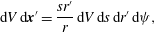 $$\begin{eqnarray}\text{d}V\,\text{d}\boldsymbol{x}^{\prime }=\frac{sr^{\prime }}{r}\,\text{d}V\,\text{d}s\,\text{d}r^{\prime }\,\text{d}{\it\psi},\end{eqnarray}$$
where
 $s=|\boldsymbol{x}-\boldsymbol{x}^{\prime }|$
, giving (2.18a
); (2.18b–d
) are obtained similarly.
Next, we provide a sketch of the derivation of (2.21), for
 $k=1$
. We note that (2.18a
) can be written as
 $$\begin{eqnarray}q_{1}(r)=\int _{0}^{\infty }\mathop{\sum }_{j=1}^{4}H_{1j}(r,r^{\prime })q_{j}(r^{\prime })\,\text{d}r^{\prime }+S_{1}(r),\end{eqnarray}$$
where
 $$\begin{eqnarray}S_{1}(r)=\frac{1}{{\rm\pi}^{3/2}}\int _{R1}\tilde{h}_{0}(\boldsymbol{x}_{0},\boldsymbol{c})\exp \left(-V^{2}-\frac{1-\text{i}{\it\Theta}}{VKn}|\boldsymbol{x}-\boldsymbol{x}_{0}|\right)\,\text{d}\boldsymbol{c}\end{eqnarray}$$
and the functions
 $H_{1j}(r,r^{\prime })$
are found by comparing (2.18a
) and (A 12). The inhomogeneous term
 $S_{1}$
in (A 12) is of the form
 $$\begin{eqnarray}S_{1}(r)=W_{1}(r)+gR_{1}(r),\end{eqnarray}$$
where
 $g$
is a constant,
 $$\begin{eqnarray}g=\sqrt{{\rm\pi}}+\int _{1}^{\infty }a_{1}(r^{\prime })q_{1}(r^{\prime })+a_{2}(r^{\prime })q_{2}(r^{\prime })+a_{3}(r^{\prime })q_{3}(r^{\prime })+a_{4}(r^{\prime })q_{4}(r^{\prime })\,\text{d}r^{\prime }.\end{eqnarray}$$
The functions
 $a_{i}(r^{\prime })$
are found by comparing (A 13) and (A 14). Combination of (A 12), (A 14) and (A 15) then gives
 $$\begin{eqnarray}q_{1}(r)=\int _{0}^{\infty }\mathop{\sum }_{j=1}^{4}[H_{1j}(r,r^{\prime })+R_{1}(r)a_{j}(r^{\prime })]q_{j}(r^{\prime })\,\text{d}r^{\prime }+W_{1}(r)-\sqrt{{\rm\pi}}R_{1}(r),\end{eqnarray}$$
which corresponds to (2.21) for
 $k=1$
, with
 $K_{1j}(r,r^{\prime })=H_{1j}(r,r^{\prime })+R_{1}(r)a_{j}(r^{\prime })$
and
 $T_{1}(r)=W_{1}(r)-\sqrt{{\rm\pi}}R_{1}(r)$
.
Appendix B. Kernels and inhomogeneous terms
To obtain simplified forms of all functions in this appendix, we use the following geometric relations:
 $$\begin{eqnarray}\displaystyle \displaystyle \cos {\it\chi} & \hspace{-2.0pt}=\hspace{-2.0pt} & \displaystyle \frac{r^{2}+s^{2}-r^{\prime 2}}{2rs},\end{eqnarray}$$
 $$\begin{eqnarray}\displaystyle \displaystyle \cos {\it\theta}^{\prime } & \hspace{-2.0pt}=\hspace{-2.0pt} & \displaystyle \frac{1}{r^{\prime }}\left(s\sin {\it\chi}\sin {\it\psi}\sin {\it\theta}+\left[r-s\cos {\it\chi}\right]\cos {\it\theta}\right),\end{eqnarray}$$
 $$\begin{eqnarray}\displaystyle \displaystyle c_{r}^{\prime } & \hspace{-2.0pt}=\hspace{-2.0pt} & \displaystyle V\frac{r^{2}-s^{2}-r^{\prime 2}}{2r^{\prime }s},\end{eqnarray}$$
 $$\begin{eqnarray}\displaystyle \displaystyle c_{{\it\theta}^{\prime }}\sin {\it\theta}^{\prime } & = & \displaystyle \frac{V}{4rr^{\prime 2}s} (\,[r^{4}+(r^{\prime 2}-s^{2})^{2}-2r^{2}(r^{\prime 2}+s^{2})]\cos {\it\theta}\nonumber\\ \displaystyle & & \displaystyle +\,2rs(r^{2}+r^{\prime 2}-s^{2})\sin {\it\chi}\sin {\it\theta}\sin {\it\psi}).\end{eqnarray}$$
 $\{c_{r},c_{{\it\theta}},c_{r^{\prime }},c_{{\it\theta}^{\prime }},\cos {\it\theta}^{\prime },\sin {\it\theta}^{\prime }\}$
in (2.18) in terms of the integration variables
 $\{r^{\prime },s,{\it\psi},V\}$
.
The kernel functions,
 $K_{km}(r,r^{\prime })$
, and inhomogeneous terms,
 $T_{k}(r)$
, in (2.21) can be written as
 $$\begin{eqnarray}K_{km}(r,r^{\prime })=H_{km}(r,r^{\prime })+R_{k}(r)a_{m}(r^{\prime })\end{eqnarray}$$
and
 $$\begin{eqnarray}T_{k}(r)=W_{k}(r)-\sqrt{{\rm\pi}}R_{k}(r)\end{eqnarray}$$
respectively, where the functions
 $H_{ij}(r,r^{\prime }),R_{k}(r),a_{m}(r^{\prime }),W_{k}(r),R_{k}(r)$
are defined explicitly for steady and unsteady flow below.
For unsteady flow, the simplified kernel functions
 $H_{ij}(r,r^{\prime })$
for
 $i,j\in \{1,2,3,4\}$
in (B 2) are
 $$\begin{eqnarray}\displaystyle \displaystyle H_{11} & \hspace{-2.0pt}=\hspace{-2.0pt} & \displaystyle \displaystyle -\frac{1}{\sqrt{{\rm\pi}}}\int \frac{1}{Kn}\frac{1}{r^{2}s}(s^{2}-r^{2}-r^{\prime 2})I_{1}\left(\frac{1-\text{i}{\it\Theta}}{Kn}s\right)\,\text{d}s,\end{eqnarray}$$
 $$\begin{eqnarray}\displaystyle \displaystyle H_{12} & \hspace{-2.0pt}=\hspace{-2.0pt} & \displaystyle \displaystyle \frac{1}{\sqrt{{\rm\pi}}}\int \frac{1}{Kn}\frac{1}{r^{2}r^{\prime }s^{2}}(s^{4}-2r^{2}s^{2}+r^{4}-r^{\prime 4})I_{2}\left(\frac{1-\text{i}{\it\Theta}}{Kn}s\right)\,\text{d}s,\end{eqnarray}$$
 $$\begin{eqnarray}\displaystyle \displaystyle H_{13} & \hspace{-2.0pt}=\hspace{-2.0pt} & \displaystyle \displaystyle \frac{1}{\sqrt{{\rm\pi}}}\int \frac{1}{Kn}\frac{1}{r^{2}r^{\prime }s^{2}}(s^{4}-2s^{2}(r^{2}+r^{\prime 2})+(r^{2}-r^{\prime 2})^{2})I_{2}\left(\frac{1-\text{i}{\it\Theta}}{Kn}s\right)\,\text{d}s,\end{eqnarray}$$
 $$\begin{eqnarray}\displaystyle \displaystyle H_{14} & \hspace{-2.0pt}=\hspace{-2.0pt} & \displaystyle \displaystyle -\frac{1}{\sqrt{{\rm\pi}}}\int \frac{1}{Kn}\frac{1}{r^{2}s}\left[I_{3}\left(\frac{1-\text{i}{\it\Theta}}{Kn}s\right)-\frac{3}{2}I_{1}\left(\frac{1-\text{i}{\it\Theta}}{Kn}s\right)\right]\left(s^{2}-r^{2}-r^{\prime 2}\right)\,\text{d}s,\end{eqnarray}$$
 $$\begin{eqnarray}\displaystyle \displaystyle H_{21} & \hspace{-2.0pt}=\hspace{-2.0pt} & \displaystyle \displaystyle -\frac{1}{\sqrt{{\rm\pi}}}\int \frac{1}{Kn}\frac{1}{2r^{3}s^{2}}(s^{4}-2r^{\prime 2}s^{2}+r^{\prime 4}-r^{4})I_{2}\left(\frac{1-\text{i}{\it\Theta}}{Kn}s\right)\,\text{d}s,\end{eqnarray}$$
 $$\begin{eqnarray}\displaystyle \displaystyle H_{22} & \hspace{-2.0pt}=\hspace{-2.0pt} & \displaystyle \displaystyle \frac{1}{\sqrt{{\rm\pi}}}\int \frac{1}{Kn}\frac{1}{2r^{3}r^{\prime }s^{3}}(s^{6}-s^{4}(r^{\prime 2}+r^{2})-s^{2}(r^{2}-r^{\prime 2})^{2}+(r^{\prime 4}-r^{4})(r^{\prime 2}-r^{2}))\nonumber\\ \displaystyle & & \displaystyle \displaystyle \times \,I_{3}\left(\frac{1-\text{i}{\it\Theta}}{Kn}s\right)\,\text{d}s,\end{eqnarray}$$
 $$\begin{eqnarray}\displaystyle \displaystyle H_{23} & \hspace{-2.0pt}=\hspace{-2.0pt} & \displaystyle \displaystyle \frac{1}{\sqrt{{\rm\pi}}}\int \frac{1}{Kn}\frac{1}{2r^{3}r^{\prime }s^{3}}(s^{6}-s^{4}(3r^{\prime 2}+r^{2})+s^{2}(3r^{\prime 2}+r^{2})(r^{\prime 2}-r^{2})-(r^{\prime 2}-r^{2})^{3})\nonumber\\ \displaystyle & & \displaystyle \displaystyle \times \,I_{3}\left(\frac{1-\text{i}{\it\Theta}}{Kn}s\right)\text{d}s,\end{eqnarray}$$
 $$\begin{eqnarray}\displaystyle \displaystyle H_{24} & \hspace{-2.0pt}=\hspace{-2.0pt} & \displaystyle \displaystyle -\frac{1}{\sqrt{{\rm\pi}}}\int \frac{1}{Kn}\frac{1}{2r^{3}s^{2}}\left[I_{4}\left(\frac{1-\text{i}{\it\Theta}}{Kn}s\right)-\frac{3}{2}I_{2}\left(\frac{1-\text{i}{\it\Theta}}{Kn}s\right)\right]\nonumber\\ \displaystyle & & \displaystyle \displaystyle \times \,\left(s^{4}-2s^{2}r^{\prime 2}+r^{\prime 4}-r^{4}\right)\,\text{d}s,\end{eqnarray}$$
 $$\begin{eqnarray}\displaystyle \displaystyle H_{31} & \hspace{-2.0pt}=\hspace{-2.0pt} & \displaystyle \displaystyle -\frac{1}{\sqrt{{\rm\pi}}}\int \frac{1}{Kn}I_{2}\left(\frac{1-\text{i}{\it\Theta}}{Kn}s\right)\frac{1}{4r^{3}s^{2}}(s^{4}-2s^{2}(r^{2}+r^{\prime 2})+(r^{\prime 2}-r^{2})^{2})\,\text{d}s,\end{eqnarray}$$
 $$\begin{eqnarray}\displaystyle \displaystyle H_{32} & \hspace{-2.0pt}=\hspace{-2.0pt} & \displaystyle \displaystyle \frac{1}{\sqrt{{\rm\pi}}}\int \frac{1}{Kn}\frac{1}{4r^{3}r^{\prime }s^{3}}(s^{6}-s^{4}(3r^{2}+r^{\prime 2})+s^{2}(3r^{2}+r^{\prime 2})(r^{2}-r^{\prime 2})-(r^{2}-r^{\prime 2})^{3})\nonumber\\ \displaystyle & & \displaystyle \displaystyle \times \,I_{3}\left(\frac{1-\text{i}{\it\Theta}}{Kn}s\right)\,\text{d}s,\end{eqnarray}$$
 $$\begin{eqnarray}\displaystyle \displaystyle H_{33} & \hspace{-2.0pt}=\hspace{-2.0pt} & \displaystyle \displaystyle \frac{1}{\sqrt{{\rm\pi}}}\int \frac{1}{Kn}(s^{6}-s^{4}(3r^{\prime 2}+3r^{2})+s^{2}(3r^{4}+2r^{2}r^{\prime 2}+3r^{\prime 4})-(r^{2}-r^{\prime 2})(r^{4}-r^{\prime 4}))\nonumber\\ \displaystyle & & \displaystyle \displaystyle \times \,\frac{1}{4r^{3}r^{\prime }s^{3}}I_{3}\left(\frac{1-\text{i}{\it\Theta}}{Kn}s\right)\,\text{d}s,\end{eqnarray}$$
 $$\begin{eqnarray}\displaystyle \displaystyle H_{34} & \hspace{-2.0pt}=\hspace{-2.0pt} & \displaystyle \displaystyle -\frac{1}{\sqrt{{\rm\pi}}}\int \frac{1}{Kn}\frac{1}{4r^{3}s^{2}}\left[I_{4}\left(\frac{1-\text{i}{\it\Theta}}{Kn}s\right)-\frac{3}{2}I_{2}\left(\frac{1-\text{i}{\it\Theta}}{Kn}s\right)\right]\nonumber\\ \displaystyle & & \displaystyle \displaystyle \times \,\left(s^{4}-2s^{2}(r^{2}+r^{\prime 2})+(r^{\prime 2}-r^{2})^{2}\right)\,\text{d}s,\end{eqnarray}$$
 $$\begin{eqnarray}\displaystyle \displaystyle H_{41} & \hspace{-2.0pt}=\hspace{-2.0pt} & \displaystyle \displaystyle {\textstyle \frac{2}{3}}H_{14},\end{eqnarray}$$
 $$\begin{eqnarray}\displaystyle \displaystyle H_{42} & \hspace{-2.0pt}=\hspace{-2.0pt} & \displaystyle \displaystyle \frac{2}{3\sqrt{{\rm\pi}}}\int \frac{1}{Kn}\frac{1}{r^{2}r^{\prime }s^{2}}\left[I_{4}\left(\frac{1-\text{i}{\it\Theta}}{Kn}s\right)-\frac{3}{2}I_{2}\left(\frac{1-\text{i}{\it\Theta}}{Kn}s\right)\right]\nonumber\\ \displaystyle & & \displaystyle \displaystyle \times \,\left(s^{4}-2s^{2}r^{2}+(r^{4}-r^{\prime 4})\right)\,\text{d}s,\end{eqnarray}$$
 $$\begin{eqnarray}\displaystyle \displaystyle H_{43} & \hspace{-2.0pt}=\hspace{-2.0pt} & \displaystyle \displaystyle \frac{2}{3\sqrt{{\rm\pi}}}\int \frac{1}{Kn}\left[I_{4}\left(\frac{1-\text{i}{\it\Theta}}{Kn}s\right)-\frac{3}{2}I_{2}\left(\frac{1-\text{i}{\it\Theta}}{Kn}s\right)\right]\nonumber\\ \displaystyle & & \displaystyle \displaystyle \times \,\frac{1}{r^{2}r^{\prime }s^{2}}(s^{4}-2s^{2}(r^{2}+r^{\prime 2})+(r^{2}-r^{\prime 2})^{2})\,\text{d}s,\end{eqnarray}$$
 $$\begin{eqnarray}\displaystyle \displaystyle H_{44} & \hspace{-2.0pt}=\hspace{-2.0pt} & \displaystyle \displaystyle -\frac{2}{3\sqrt{{\rm\pi}}}\int \frac{1}{Kn}\frac{1}{r^{2}s}\left[I_{5}\left(\frac{1-\text{i}{\it\Theta}}{Kn}s\right)-3I_{3}\left(\frac{1-\text{i}{\it\Theta}}{Kn}s\right)+\frac{9}{4}I_{1}\left(\frac{1-\text{i}{\it\Theta}}{Kn}s\right)\right]\nonumber\\ \displaystyle & & \displaystyle \displaystyle \times \,\left(s^{2}-r^{2}-r^{\prime 2}\right)\,\text{d}s,\end{eqnarray}$$
 $s\in [|r-r^{\prime }|,\sqrt{r^{2}-1}+\sqrt{r^{\prime 2}-1}]$
and
 $I_{n}(z)$
is the Abramowitz function:
 $$\begin{eqnarray}I_{n}(x)=\int _{0}^{\infty }{\it\zeta}^{n}\exp \left(-{\it\zeta}^{2}-\frac{x}{{\it\zeta}}\right)\,\text{d}{\it\zeta}.\end{eqnarray}$$
For steady flow,
 ${\it\Theta}$
is set to zero in (B 4), which then coincides with the (steady) results of Lea & Loyalka (Reference Lea and Loyalka1982) and Law & Loyalka (Reference Law and Loyalka1986), apart from typographical errors.
For unsteady flow, the functions
 $a_{i}$
,
 $W_{i}$
and
 $R_{i}$
for
 $i\in \{1,2,3,4\}$
are
 $$\begin{eqnarray}\displaystyle \displaystyle a_{1}(r^{\prime }) & \hspace{-2.0pt}=\hspace{-2.0pt} & \displaystyle \displaystyle \int _{r^{\prime }-1}^{\sqrt{r^{\prime 2}-1}}\frac{1}{Kn}\frac{1}{p^{2}}(p^{4}-2p^{2}r^{\prime 2}+(r^{\prime 4}-1))I_{2}\left(\frac{1-\text{i}{\it\Theta}}{Kn}p\right)\,\text{d}p,\end{eqnarray}$$
 $$\begin{eqnarray}\displaystyle \displaystyle a_{2}(r^{\prime }) & \hspace{-2.0pt}=\hspace{-2.0pt} & \displaystyle \displaystyle -\int _{r^{\prime }-1}^{\sqrt{r^{\prime 2}-1}}\frac{1}{Kn}\frac{1}{r^{\prime }p^{3}}(p^{6}-p^{4}(r^{\prime 2}+1)-p^{2}(r^{\prime 2}-1)^{2}+(r^{\prime 4}-1)(r^{\prime 2}-1))\nonumber\\ \displaystyle & & \displaystyle \displaystyle \times \,I_{3}\left(\frac{1-\text{i}{\it\Theta}}{Kn}p\right)\,\text{d}p,\end{eqnarray}$$
 $$\begin{eqnarray}\displaystyle \displaystyle a_{3}(r^{\prime }) & \hspace{-2.0pt}=\hspace{-2.0pt} & \displaystyle \displaystyle -\int _{r^{\prime }-1}^{\sqrt{r^{\prime 2}-1}}\frac{1}{Kn}\frac{1}{r^{\prime }p^{3}}(p^{6}-p^{4}(3r^{\prime 2}+1)+p^{2}(3r^{\prime 2}+1)(r^{\prime 2}-1)-(r^{\prime 2}-1)^{3})\nonumber\\ \displaystyle & & \displaystyle \displaystyle \times \,I_{3}\left(\frac{1-\text{i}{\it\Theta}}{Kn}p\right)\,\text{d}p,\end{eqnarray}$$
 $$\begin{eqnarray}\displaystyle \displaystyle a_{4}(r^{\prime }) & \hspace{-2.0pt}=\hspace{-2.0pt} & \displaystyle \displaystyle \int _{r^{\prime }-1}^{\sqrt{r^{\prime 2}-1}}\frac{1}{Kn}\frac{1}{p^{2}}\left[I_{4}\left(\frac{1-\text{i}{\it\Theta}}{Kn}p\right)-\frac{3}{2}I_{2}\left(\frac{1-\text{i}{\it\Theta}}{Kn}p\right)\right]\nonumber\\ \displaystyle & & \displaystyle \displaystyle \times \,\left(p^{4}-2p^{2}r^{\prime 2}+(r^{\prime 4}-1)\right)\,\text{d}p,\end{eqnarray}$$
 $$\begin{eqnarray}\displaystyle \displaystyle W_{1}(r) & \hspace{-2.0pt}=\hspace{-2.0pt} & \displaystyle \displaystyle -\frac{1}{\sqrt{{\rm\pi}}}\int _{r-1}^{\sqrt{r^{2}-1}}\frac{1}{r^{2}l^{3}}\left(l^{4}-(r^{2}-1)^{2}\right)I_{3}\left(\frac{1-\text{i}{\it\Theta}}{Kn}l\right)\,\text{d}l,\end{eqnarray}$$
 $$\begin{eqnarray}\displaystyle \displaystyle W_{2}(r) & \hspace{-2.0pt}=\hspace{-2.0pt} & \displaystyle \displaystyle -\frac{1}{\sqrt{{\rm\pi}}}\int _{r-1}^{\sqrt{r^{2}-1}}\frac{1}{2r^{3}l^{4}}\left(l^{6}+l^{4}(r^{2}-1)-l^{2}(r^{2}-1)^{2}-(r^{2}-1)^{3}\right)\nonumber\\ \displaystyle & & \displaystyle \times \,I_{4}\left(\frac{1-\text{i}{\it\Theta}}{Kn}l\right)\,\text{d}l,\end{eqnarray}$$
 $$\begin{eqnarray}\displaystyle \displaystyle W_{3}(r) & \hspace{-2.0pt}=\hspace{-2.0pt} & \displaystyle \displaystyle -\frac{1}{\sqrt{{\rm\pi}}}\int _{r-1}^{\sqrt{r^{2}-1}}\frac{1}{4r^{3}l^{4}}(l^{6}-l^{4}(3r^{2}+1)+l^{2}(3r^{2}+1)(r^{2}-1)-(r^{2}-1)^{3})\nonumber\\ \displaystyle & & \displaystyle \displaystyle \times \,I_{4}\left(\frac{1-\text{i}{\it\Theta}}{Kn}l\right)\,\text{d}l,\end{eqnarray}$$
 $$\begin{eqnarray}\displaystyle \displaystyle W_{4}(r) & \hspace{-2.0pt}=\hspace{-2.0pt} & \displaystyle \displaystyle -\frac{2}{3\sqrt{{\rm\pi}}}\int _{r-1}^{\sqrt{r^{2}-1}}\frac{1}{r^{2}l^{3}}\left[I_{5}\left(\frac{1-\text{i}{\it\Theta}}{Kn}l\right)-\frac{3}{2}I_{3}\left(\frac{1-\text{i}{\it\Theta}}{Kn}l\right)\right](l^{4}-(1-r^{2})^{2})\,\text{d}l,\nonumber\\ \displaystyle & & \displaystyle\end{eqnarray}$$
 $$\begin{eqnarray}\displaystyle \displaystyle R_{1}(r) & \hspace{-2.0pt}=\hspace{-2.0pt} & \displaystyle \displaystyle \frac{1}{\sqrt{{\rm\pi}}}\int _{r-1}^{\sqrt{r^{2}-1}}\frac{1}{2r^{2}l^{2}}(l^{4}-2l^{2}r^{2}+r^{4}-1)I_{2}\left(\frac{1-\text{i}{\it\Theta}}{Kn}l\right)\,\text{d}l,\end{eqnarray}$$
 $$\begin{eqnarray}\displaystyle \displaystyle R_{2}(r) & \hspace{-2.0pt}=\hspace{-2.0pt} & \displaystyle \displaystyle \frac{1}{\sqrt{{\rm\pi}}}\int _{r-1}^{\sqrt{r^{2}-1}}\frac{1}{4r^{3}l^{3}}(l^{6}-l^{4}(r^{2}+1)-l^{2}(r^{2}-1)^{2}+(r^{2}-1)^{2}(r^{2}+1))\nonumber\\ \displaystyle & & \displaystyle \displaystyle \times \,I_{3}\left(\frac{1-\text{i}{\it\Theta}}{Kn}l\right)\,\text{d}l,\end{eqnarray}$$
 $$\begin{eqnarray}\displaystyle \displaystyle R_{3}(r) & \hspace{-2.0pt}=\hspace{-2.0pt} & \displaystyle \displaystyle \frac{1}{\sqrt{{\rm\pi}}}\int _{r-1}^{\sqrt{r^{2}-1}}\frac{1}{8r^{3}l^{3}}(l^{6}-l^{4}(3r^{2}+1)+l^{2}(3r^{2}+1)(r^{2}-1)-(r^{2}-1)^{3})\nonumber\\ \displaystyle & & \displaystyle \displaystyle \times \,I_{3}\left(\frac{1-\text{i}{\it\Theta}}{Kn}l\right)\,\text{d}l,\end{eqnarray}$$
 $$\begin{eqnarray}\displaystyle \displaystyle R_{4}(r) & \hspace{-2.0pt}=\hspace{-2.0pt} & \displaystyle \displaystyle \frac{2}{3\sqrt{{\rm\pi}}}\int _{r-1}^{\sqrt{r^{2}-1}}\frac{1}{2r^{2}l^{2}}\left[I_{4}\left(\frac{1-\text{i}{\it\Theta}}{Kn}l\right)-\frac{3}{2}I_{2}\left(\frac{1-\text{i}{\it\Theta}}{Kn}l\right)\right]\nonumber\\ \displaystyle & & \displaystyle \displaystyle \times \,(l^{4}-2l^{2}r^{2}+(r^{4}-1))\,\text{d}l.\end{eqnarray}$$
 ${\it\Theta}$
is again set to zero in (B 6); these results then coincide with those of Lea & Loyalka (Reference Lea and Loyalka1982) and Law & Loyalka (Reference Law and Loyalka1986).
Functions containing a subscript ‘4’ in (B 4) and (B 6) arise in the non-isothermal problem and are reported in Law & Loyalka (Reference Law and Loyalka1986); all other functions are identical to those in Lea & Loyalka (Reference Lea and Loyalka1982).
Appendix C. Unsteady free-molecular flow
The functions
 $\bar{W}_{i}$
and
 $\bar{R}_{i}$
for
 $i\in \{1,2,3,4\}$
are used in the solution for unsteady free-molecular flow, see (3.10), and are defined as
 $$\begin{eqnarray}\displaystyle \displaystyle \bar{W}_{1}(r) & \hspace{-2.0pt}=\hspace{-2.0pt} & \displaystyle \displaystyle -\frac{1}{\sqrt{{\rm\pi}}}\int _{r-1}^{\sqrt{r^{2}-1}}\frac{1}{r^{2}l^{3}}\left(l^{4}-(r^{2}-1)^{2}\right)I_{3}\left(-\frac{\text{i}{\it\Theta}}{Kn}l\right)\,\text{d}l,\end{eqnarray}$$
 $$\begin{eqnarray}\displaystyle \displaystyle \bar{W}_{2}(r) & \hspace{-2.0pt}=\hspace{-2.0pt} & \displaystyle \displaystyle -\frac{1}{\sqrt{{\rm\pi}}}\int _{r-1}^{\sqrt{r^{2}-1}}\frac{1}{2r^{3}l^{4}}\left(l^{6}+l^{4}(r^{2}-1)-l^{2}(r^{2}-1)^{2}-(r^{2}-1)^{3}\right)\nonumber\\ \displaystyle & & \displaystyle \displaystyle \times \,I_{4}\left(-\frac{\text{i}{\it\Theta}}{Kn}l\right)\,\text{d}l,\end{eqnarray}$$
 $$\begin{eqnarray}\displaystyle \displaystyle \bar{W}_{3}(r) & \hspace{-2.0pt}=\hspace{-2.0pt} & \displaystyle \displaystyle -\frac{1}{\sqrt{{\rm\pi}}}\int _{r-1}^{\sqrt{r^{2}-1}}\frac{1}{4r^{3}l^{4}}(l^{6}-l^{4}(3r^{2}+1)+l^{2}(3r^{2}+1)(r^{2}-1)-(r^{2}-1)^{3})\nonumber\\ \displaystyle & & \displaystyle \displaystyle \times \,I_{4}\left(-\frac{\text{i}{\it\Theta}}{Kn}l\right)\,\text{d}l,\end{eqnarray}$$
 $$\begin{eqnarray}\displaystyle \displaystyle \bar{W}_{4}(r) & \hspace{-2.0pt}=\hspace{-2.0pt} & \displaystyle \displaystyle -\frac{2}{3\sqrt{{\rm\pi}}}\int _{r-1}^{\sqrt{r^{2}-1}}\frac{1}{r^{2}l^{3}}\left[I_{5}\left(-\frac{\text{i}{\it\Theta}}{Kn}l\right)-\frac{3}{2}I_{3}\left(-\frac{\text{i}{\it\Theta}}{Kn}l\right)\right](l^{4}-(1-r^{2})^{2})\,\text{d}l,\nonumber\\ \displaystyle & & \displaystyle\end{eqnarray}$$
 $$\begin{eqnarray}\displaystyle \displaystyle \bar{R}_{1}(r) & \hspace{-2.0pt}=\hspace{-2.0pt} & \displaystyle \displaystyle \frac{1}{\sqrt{{\rm\pi}}}\int _{r-1}^{\sqrt{r^{2}-1}}\frac{1}{2r^{2}l^{2}}(l^{4}-2l^{2}r^{2}+r^{4}-1)I_{2}\left(-\frac{\text{i}{\it\Theta}}{Kn}l\right)\,\text{d}l,\end{eqnarray}$$
 $$\begin{eqnarray}\displaystyle \displaystyle \bar{R}_{2}(r) & \hspace{-2.0pt}=\hspace{-2.0pt} & \displaystyle \displaystyle \frac{1}{\sqrt{{\rm\pi}}}\int _{r-1}^{\sqrt{r^{2}-1}}\frac{1}{4r^{3}l^{3}}(l^{6}-l^{4}(r^{2}+1)-l^{2}(r^{2}-1)^{2}+(r^{2}-1)^{2}(r^{2}+1))\nonumber\\ \displaystyle & & \displaystyle \displaystyle \times \,I_{3}\left(-\frac{\text{i}{\it\Theta}}{Kn}l\right)\,\text{d}l,\end{eqnarray}$$
 $$\begin{eqnarray}\displaystyle \displaystyle \bar{R}_{3}(r) & \hspace{-2.0pt}=\hspace{-2.0pt} & \displaystyle \displaystyle \frac{1}{\sqrt{{\rm\pi}}}\int _{r-1}^{\sqrt{r^{2}-1}}\frac{1}{8r^{3}l^{3}}(l^{6}-l^{4}(3r^{2}+1)+l^{2}(3r^{2}+1)(r^{2}-1)-(r^{2}-1)^{3})\nonumber\\ \displaystyle & & \displaystyle \displaystyle \times \,I_{3}\left(-\frac{\text{i}{\it\Theta}}{Kn}l\right)\,\text{d}l,\end{eqnarray}$$
 $$\begin{eqnarray}\displaystyle \displaystyle \bar{R}_{4}(r) & \hspace{-2.0pt}=\hspace{-2.0pt} & \displaystyle \displaystyle \frac{2}{3\sqrt{{\rm\pi}}}\int _{r-1}^{\sqrt{r^{2}-1}}\frac{1}{2r^{2}l^{2}}\left[I_{4}\left(-\frac{\text{i}{\it\Theta}}{Kn}l\right)-\frac{3}{2}I_{2}\left(-\frac{\text{i}{\it\Theta}}{Kn}l\right)\right]\nonumber\\ \displaystyle & & \displaystyle \displaystyle \times \,(l^{4}-2l^{2}r^{2}+(r^{4}-1))\,\text{d}l.\end{eqnarray}$$
Appendix D. Numerical convergence procedure
D.1 Steady flow
For steady flow, the integration domain is divided into three subdomains,
 $[1,R_{L}]$
,
 $[R_{L},R_{M}]$
and
 $[R_{M},R_{N}]$
; see figure 4. A dense grid of size
 $N_{1}L_{1}$
is applied to the subdomain
 $[1,R_{L}]$
, while a coarse grid of size
 $N_{2}L_{2}$
is applied to the subdomain
 $[R_{L},R_{M}]$
. In the subdomain furthest from the sphere,
 $[R_{M},R_{N}]$
, we apply quadrature of order
 $N_{c}$
. Additionally, we choose
 $R_{L}=1+Kn$
,
 $N_{1}=10$
and
 $N_{2}=5$
. The following steps are implemented to obtain convergence.
-
(i) First, we systematically increase
$R_{M}$
while keeping
$L_{1}$
,
$\text{d}r_{2}=(R_{M}-R_{L})/(N_{2}L_{2})$
and
$R_{N}/R_{M}$
fixed. Values for
$\text{d}r_{3}=(R_{N}-R_{M})/N_{c}$
in this case are chosen to be approximately identical, although small-
$R_{M}$
simulations require a slightly denser discretisation. This allows convergence to be assessed as the domain is increased. The value of
$R_{M}$
is increased until convergence of the force on the sphere is achieved. Convergence is obtained to at least four decimal places, where possible. (Finite computational resources limit the precision of solutions, hence the accuracy of solutions varies for different Knudsen numbers and frequency ratios.) -
(ii) Second,
$L_{1}$
is doubled and
$L_{2}$
is systematically increased (thereby decreasing the average spacing
$\text{d}r_{2}$
) while keeping
$R_{M}$
,
$R_{N}/R_{M}$
and
$\text{d}r_{3}$
fixed. Convergence is assessed as the quadrature order within the subdomain
$[1,R_{M}]$
is increased. The value of
$L_{2}$
is fixed when convergence of the force is obtained; convergence properties similar to (i). -
(iii) Third, the ratio
$R_{N}/R_{M}$
is increased while the average spacing
$\text{d}r_{3}$
is kept fixed. All other computational parameters are also held constant. This allows convergence to be assessed as the domain in which the asymptotic solution is applied is expanded. The value of
$R_{N}/R_{M}$
is fixed when convergence of the force is achieved. Convergence to more than four decimal places is typically obtained. -
(iv) Finally, the quadrature order
$N_{c}$
is systematically increased (and therefore
$\text{d}r_{3}$
is decreased) to assess the effect of the quadrature order in the (far-field) asymptotic region. This effect is small because the flow is near-continuum in this region, and therefore varies very smoothly with respect to the radius
$r$
. The value of
$N_{c}$
is fixed when convergence of the force is achieved; convergence similar to (iii) is obtained.







Different computational parameters
 $R_{L}$
,
 $R_{M}$
,
 $R_{N}$
,
 $L_{1}$
and
 $L_{2}$
are used for each Knudsen number. As an example, results for these values, for
 $Kn=1$
, are given in table 3.
Table 4 gives the normalised force on the sphere
 $\tilde{F}/\tilde{F}_{fm}$
(see (2.25) and (3.11)) for different computational parameters and
 $Kn=1$
. Each progressive part (from (a) to (d)) in table 4 shows how the calculated force varies as a single computational parameter is systematically adjusted while other computational parameters are held fixed. In each part, the force converges to four significant figures. The radius
 $r=R_{M}$
and quadrature order
 $N_{2}$
(via
 $\text{d}r_{2}$
, see the definition in the caption of table 3) used in the domain
 $[R_{L},R_{M}]$
have the most significant impact on accuracy. These results show that the presented numerical results are insensitive to the computational parameters
 $R_{N}/R_{M}$
and
 $N_{c}$
. The weak dependence of the accuracy on
 $R_{N}/R_{M}$
and
 $N_{c}$
may be due to the original values being sufficient for accurate computation. It does not necessarily imply that extending the computational domain via the use of asymptotic solutions does not improve the accuracy. In fact, we find that choosing
 $R_{M}=R_{N}$
yields slow convergence of the solutions.
Steady flow: computational parameters used to verify convergence for
 $Kn=1$
, where
 $\text{d}r_{2}=(R_{M}-R_{L})/(N_{2}L_{2})$
and
 $\text{d}r_{3}=(R_{N}-R_{M})/N_{c}$
.

Steady flow: convergence of the normalised force
 $\tilde{F}/\tilde{F}_{fm}$
for
 $Kn=1$
as (a)
 $R_{M}$
is increased, followed by (b) decrease in the average mesh spacing
 $\text{d}r_{2}$
, followed by (c) increase of
 $R_{N}/R_{M}$
, followed by (d) increase of the quadrature order
 $N_{c}$
. The force converges to four significant figures. At each step in this sequence, values for all other parameters are listed in table 3. The largest relative difference between solutions generated with different computational parameters is
 $0.001\,\%$
.
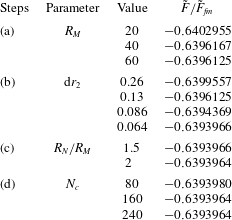
Similar convergence is obtained for
 $Kn=0.1,0.3,2,3,10$
, where the numerical results converge to four significant figures. For
 $Kn=0.1$
, the largest percentage relative difference is 0.003 %, while for
 $Kn=10$
, the largest percentage relative difference is 0.0001 %.
D.2 Unsteady flow
For unsteady flow, the integration domain is divided into two subdomains,
 $[1,R_{L}]$
and
 $[R_{L},R_{M}]$
; see figure 4. A dense grid of size
 $N_{1}L_{1}$
is applied to the subdomain
 $[1,R_{L}]$
while a coarse grid of size
 $N_{2}L_{2}$
is applied to
 $[R_{L},R_{M}]$
. For unsteady flow,
 $R_{L}$
is chosen to be
 $1+Kn$
or
 $1+Kn/{\it\Theta}$
depending on which is the smallest dominant length scale. Additionally,
 $N_{1}=10$
and
 $N_{2}=5$
.
The radius
 $R_{M}$
is varied with all other parameters held fixed. Then, similarly,
 $L_{2}$
is adjusted with all other parameters kept constant; see steps (a) and (b) for steady flow in § D.1. Table 5 shows the computational parameters used for two cases, (
 $Kn=1$
,
 ${\it\Theta}=1$
) and (
 $Kn=0.1$
,
 ${\it\Theta}=0.1$
).
Unsteady flow: computational parameters used to verify convergence as a function of
 $Kn$
and
 ${\it\Theta}$
, where
 $\text{d}r_{2}=(R_{M}-R_{L})/(N_{2}L_{2})$
.
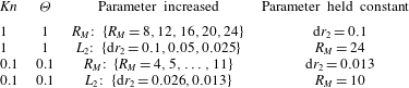
Unsteady flow: convergence of the normalised force
 $\tilde{F}/\tilde{F}_{fm}$
as a function of
 $Kn$
and
 ${\it\Theta}$
as (a)
 $R_{M}$
is increased, followed by (b) decrease in the average mesh spacing
 $\text{d}r_{2}$
. For
 $Kn=0.1$
and
 ${\it\Theta}=0.1$
, the truncation error is more dominant (relative to
 $Kn=1$
), and the force oscillates with decreasing magnitude as the parameters are refined. The estimated errors in this case are
 $2.7\,\%$
and
 $6.3\,\%$
for the real and imaginary parts respectively. This is due to steep gradients near the surface of the sphere. See table 5 for the set of computational parameters used.
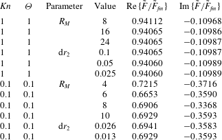
We also present a sample of the convergence achieved following the procedure in § D.1 when applied to unsteady flow. Table 6 gives the normalised force with different computational parameters for the cases (
 $Kn=1,{\it\Theta}=1$
) and (
 $Kn=0.1,{\it\Theta}=0.1$
). This shows how the result changes as one computational parameter is systematically varied while other computational parameters are kept fixed. Table 6 shows that the force results for (
 $Kn=1,{\it\Theta}=1$
) converge to five significant figures. On the other hand, the force in the near-continuum region (
 $Kn=0.1,{\it\Theta}=0.1$
) converges much slower and the solution oscillates, albeit with decreasing magnitude. The estimated relative errors in this case (measured by the magnitude of the oscillation) are 2.7 % for the real part of the force and 6.3 % for the imaginary part of the force. This is due to strong gradients in the transport variables in the vicinity of the surface, characteristic of all near-equilibrium flows and the slow far-field decay of quasi-steady (Stokes) flows.