1. Introduction
Microscale manipulation has recently opened new frontiers in biomedical and industrial applications. Targeted drug delivery [Reference Martel, Felfoul, Mathieu, Chanu, Tamaz, Mohammadi, Mankiewicz and Tabatabaei1, Reference Nelson, Kaliakatsos and Abbott2], microsurgery [Reference Ongaro, Pane, Scheggi and Misra3], microprinting [Reference Giltinan, Sridhar, Bozuyuk, Sheehan and Sitti4], and microfluidics [Reference Fan, Dong, Karacakol, Xie and Sitti5 Reference Şahin, Çetin and Özer,6] are few examples of what can be achieved by utilizing such technology. Nevertheless, designing a micro-device and its actuation system is a true challenge due to the size limitation of the micro-device [Reference Pernette, Henein, Magnani and Clavel7, Reference Shimoyama, Yasuda, Miura, Kubo Fujisawa and Ezura8]. Among the actuation systems [Reference Ceylan, Giltinan, Kozielski and Sitti9, Reference Kortschack, Shirinov, Trüper and Fatikow10], the electromagnetic actuators (EMA) have received the most attention due to their relatively simpler structure and easiness in implementation at different scales [Reference Xu, Yu, Yan, Choi and Zhang11, Reference Ebrahimi, Bi, Cappelleri, Ciuti, Conn, Faivre, Habibi, Hošovsky, Iacovacci, I. and Khalil12].
The motion of a magnetic microrobot can be controlled with an EMA system by manipulating, spatially or/and temporally [Reference Tottori, Zhang, Qiu, Krawczyk, Franco-Obregõn and Nelson13], the form of an induced magnetic field at appropriate intensity and gradient. The magnetic field, in turn, applies on the microrobot electromagnetic torque
 $\vec{\tau }$
and force
 $\vec{F}$
, which are defined as
 \begin{equation} \vec{\tau }=V(\vec{M}\times \vec{B}) \end{equation}
 \begin{equation} \vec{F}=V(\vec{M}.\nabla )\vec{B} \end{equation}
where
 $V$
,
 $\vec{M}$
, and
 $\vec{B}$
are the volume of the magnetized part of the microrobot, its magnetization vector, and magnetic flux density of the induced field, respectively. The temporal manipulations apply a rotating [Reference Xu, Hwang, Andreff and Régnier14] or an oscillating field [Reference Mahoney and Abbott15]. Therefore, a part of the microrobot should be specially designed to convert the rotational motion into translational, similar to helical micro-swimmers [Reference Xu, Hwang, Andreff and Régnier14, Reference Mahoney and Abbott15]. Such systems require complex characterizing routines [Reference Xu, Hwang, Andreff and Régnier16] and specific locomotion strategies to be developed [Reference Xu, Hwang, Andreff and Régnier14, Reference Mahoney and Abbott17]. Spatial manipulations, on the other hand, apply structured magnetic gradient for directed propulsion. Hence, the microrobots do not require any special body part for locomotion, which gives more freedom for its implementation design and simpler control models [Reference Xu, Yu, Yan, Choi and Zhang11]. Nevertheless, the sophisticated combination of both enables smoother microrobot manipulation and velocity control [Reference Hajiaghajani, Kim, Abdolali and Ahn18].
Based on these principles, different configurations of EMA systems have been proposed. These configurations were constructed mainly with Maxwell coil, Helmholtz coil, a combination of both, saddle coils or a group of electromagnets [Reference Xu, Yu, Yan, Choi and Zhang11, Reference Chen, Folio and Ferreira19]. The design of such systems is carried out by first defining the workspace of the microrobot. Then the magnetic field and its spatial and/or temporal deformation is formed by integrating the contribution of each source (coil/electromagnet) at calculated currents [Reference Choi, Choi, Jeong, Park, Ko, Park and Park20]. At the early stage of EMA systems, the studies were limited to planar manipulation of single microrobot. However, as the number of the manipulated microrobots [Reference Xie, Fan, Sun, Lin, He and Sun21] and the spatial dimensions of actuation increase, the structure of the EMA system becomes more complicated [Reference Go, Choi, Jeong, Lee, Ko, Park and Park22] since a 3D EMA system with multimagnetic sources is required to provide magnetic field control at every point of a working volume (3D workspace) [Reference Petruska and Nelson23]. For instance, the works on Octomag [Reference Kummer, Abbott, Kratochvil, Borer, Sengul, Nelson, Kummer, Abbott, Borer, Ergeneman and Nelson24, Reference Diller, Giltinan, Lum, Ye and Sitti25], Minimag [Reference Kim, Choi and Kim26], and BigMag [Reference Sikorski, Dawson, Denasi, Hekman and Misra27], which are hemispherical-shaped electromagnetic actuators, can best describe the high level of complexity. The main hindrance of this type of EMA systems is their stationary position or rotating around a fixed axis, which leads to limitations in the workspace and capability of force control due to the rapid decay of magnetic field strength with the increasing distance from the source [Reference Abbott, Peyer, Lagomarsino, Zhang, Dong, Kaliakatsos and Nelson28].
To overcome the workspace limitation, the principle of moving magnetic source actuator has been suggested. The main idea of this principle is the limited workspace can be extended if the magnetic field source is moved via an external manipulator. Based on this, several groups introduced setups in which the structure of magnetic actuator is integrated to a robotic manipulator as an end effector. However, the setups are based on permanent magnets due to their compact form and availability in a wide range of characteristics (geometry and magnetic field magnitudes). The robotic endoscopic navigation setup of Ciuti et al. [Reference Ciuti, Donlin, Valdastri, Arezzo, Menciassi, Morino and Dario29] and Tognarelli et al. [Reference Tognarelli, Castelli, Ciuti, Di Natali, Sinibaldi, Dario and Menciassi30] is an example of equipping a permanent magnet as an end effector of an industrial robotic arm. Abbott and his group developed a similar actuation principle based on rotating the magnetic field [Reference Fountain, Kailat and Abbott31]. The microrobotic actuation capabilities of this design were demonstrated [Reference Wright, Mahoney, Popek and Abbott32] with performance evaluation for prospective biomedical applications. Nevertheless, the demonstrated permanent magnet systems have the disadvantage of uncontrolled magnetic interaction between the permanent magnet and the controlled micro-object during engagement and disengagement from the permanent magnet actuators. In order to generate both attraction and repulsion forces similar to electromagnets, the two permanent magnet setup is suggested [Reference Amokrane, Belharet, Souissi and Ferreira33]. The suggested system exploits Lagrange points arising from the interference of two fields to create bidirectional magnetic gradient distribution in the vicinity of the workspace. By integrating this setup to an industrial robot arm, the researchers offer a push-pull motion control strategy for an intracochlear drug delivery microrobot [Reference Amokrane, Belharet, Souissi, Grayeli and Ferreira34]. Although the proposed system is superior to the single magnet gradient pulling systems, it also has the drawback of uncontrolled forces during the engagement and disengagement due to the usage of permanent magnets.
The rapid development of micromanipulation applications requires more versatile actuators with flexible force control. Motivated by that, we propose the idea of integrating an EMA system to a robotic arm. The essential concept was first introduced briefly as a baseline for designing special electromagnets in a previous work of us [Reference Alasli, Çetin, Akçura, Kahveci, Can and Tamer35] without focusing on the system itself. In this work, the EMA system is further investigated and developed in term of enhancing the force control flexibility, integrating a close loop control system with the aid of task space vision feedback system, and manipulating a microropbot in a complex 3D path at the microscale.
The rest of the paper is organized as follows. The following Section 2 introduces the dynamical EMA system and the function of its parts. Section 3 analyzes numerically the induced electromagnetic field and the correlation between the magnitude of the magnetic force and the symmetrical/asymmetrical configuration of the coaxial pair as positioning problem. The control strategy and systems are explained in Section 4. The last section is devoted for introducing the actuator prototype and for validating the performance of the system with a set of experiments (Section 5).
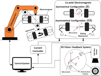
Schematic diagram of the proposed untethered EMA system [Reference Alasli, Çetin, Akçura, Kahveci, Can and Tamer35].

2. Principle of Actuation of the Untethered EMA System
The main principle of the proposed EMA system is illustrated in Fig. 1 and demonstrated in the supplemental video. The system consists of a pair of electromagnets mounted as an end effector of an industrial robotic arm. The pair is placed symmetrically face to face on one axis. The symmetric configuration (quasi-Helmholtz coil) with a precalculated distance between the pair induces a homogeneous magnetic field. Nonetheless, the distance between them can also be adjusted asymmetrically by a precise mechanism in order to form a gradient in the magnetic filed (asymmetric configuration). Hence, with this reconfiguration capability, the pair is capable of inducing either an electromagnetic torque
 $\vec{\tau }$
at the symmetric configuration or a controlled force
 $\vec{F}$
, at the asymmetric configuration, whose magnitude can be set by positioning the moving electromagnets with respect to each other at defined distances. This coaxial arrangement can control an object only on the axis of the pair by keeping in mind the following two facts of Eqs. (1) and (2),
To align a microrobot in any arbitrary direction, a homogeneous magnetic field vector (
 $\vec{B}$
) should be applied in that direction.
To propel a microrobot in any arbitrary direction, a magnetic field gradient (
$\nabla \vec{B}$
) should be applied in that direction.


The function of the robotic arm is to extend the controlled workspace from 1D to 3D by directing the applied
 $\vec{F}$
and
 $\vec{\tau }$
. This can be achieved by transporting the coaxial pair of electromagnets at 5 DOF at designed sequences according to the desired motion of the controlled object. A position-based control system is used to synchronize the motion of the robotic arm and the magnitude of
 $\vec{F}$
according to the real-time position of the controlled object in the workspace, which is received as a feedback from a 3D vision system.
3. Magnetic Force and Torque Arising from the Coaxial Pair of Electromagnets
As mentioned previously, the pair of the coaxial electromagnets can generate the required force
 $\vec{F}$
and torque
 $\vec{\tau }$
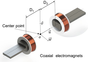
for microrobot manipulation by alternating between the asymmetric and symmetric configurations. Figure 2 illustrates a schematic diagram of two specially designed electromagnets according to the constraints of the proposed system [Reference Alasli, Çetin, Akçura, Kahveci, Can and Tamer35] placed face to face on the same axis. Each of the electromagnets can freely move along its coaxis to a specified distance from the center
 $D_1$
and
 $D_2$
. The unit vector of the coaxis is defined as
 $\vec{u}$
, where
 $\vec{u}$
,
 $\vec{v}$
, and
 $\vec{w}$
are the unit vectors of the coordinate frame placed on the center point
 $O$
.
Coaxial pair of electromagnets for inducing spatial force and torque.

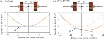
Magnetic flux density between the electromagnets on the central axis in (a) symmetric configuration and (b) asymmetric configuration.

The symmetric configuration of the electromagnets (
 $D_1=D_2$
) induces a homogeneous magnetic field (
 $\vec{B}$
) similar to Helmholtz coil at the center area of the region of interest (ROI), which is represented by the point
 $O$
for simplicity, as shown in Fig. 3(a). The homogeneous area of ROI is defined where the magnetic field intensity is deviated less than 5% of
 $\vec{B}$
at center point
 $O$
. Due to the symmetry and the design of the electromagnets, the magnetic field vector
 $\vec{B}$
on the coaxis is aligned with
 $\vec{u}$
. By assuming that the microrobot is placed at
 $O$
, the magnetic torque acting on the microrobot to align its magnetization vector
 $\vec{M}$
with
 $\vec{u}$
can be written in Eq. (3),
 \begin{equation} \vec{\tau }=V|\vec{B}|(\vec{M}\times \vec{u}) \end{equation}
On the other hand, the magnetic force can be simplified as in Eq. (4) if the rotation of the microrobot is assumed to be instantaneous,
 \begin{equation} \vec{F}=V|\vec{M}|\left(\frac{\partial B}{\partial u}\vec{u}+\frac{\partial B}{\partial v}\vec{v}+\frac{\partial B}{\partial w}\vec{w}\right) \end{equation}
An axial electromagnetic field gradient at
 $O$
(in
 $\vec{u}$
direction) is also possible to be obtained by manipulating the structural parameters of the electromagnets and by considering their dimensions are much larger than of the controlled object [Reference Alasli, Çetin, Akçura, Kahveci, Can and Tamer35]. Hence, the force equation can be further simplified to Eq. (5),
 \begin{equation} \vec{F}=V|\vec{M}|\left(\frac{\partial B}{\partial u}\vec{u}\right) \end{equation}
At the symmetric configuration,
 $\nabla _u\vec{B}$
at
 $O$
is zero and consequently the magnitude of
 $\vec{F}$
acting on the microrobot located at that point is also zero. To create a gradient at
 $O$
, we are proposing to shift one of the electromagnets relatively to the other. In other words, the distance of each electromagnet from the microrobot (at
 $O$
) becomes unequal (i.e.,
 $D_1=D+\epsilon$
and
 $D_2=D$
), where
 $\epsilon$
is the asymmetry parameter. By this means, a magnetic field gradient is created at
 $O$
, as shown in Fig. 3(b). The magnitude of
 $\nabla _u\vec{B}$
is proportional to
 $\epsilon$
. Therefore, the magnitude of
 $\vec{F}$
can be controlled by changing
 $\epsilon$
. Moreover, the direction of
 $\vec{F}$
can be set by orienting the axis of the pair of electromagnets (
 $\vec{u}$
) in space by the robotic arm which can also be true for the case of
 $\vec{\tau }$
. It is worth mentioning here that another way of generating
 $\nabla _u\vec{B}$
and controlling the magnitude of
 $\vec{F}$
can be achieved by changing the current intensity of a single or both electromagnets at the symmetric configuration. Nevertheless, due to the accompanied complexity in term of modeling, calibration, and control stability, especially for 3D manipulation, changing
 $\epsilon$
based method is utilized.
3.1. Numerical analysis of symmetric and asymmetric configurations
To understand how positioning the electromagnets affects the induced magnetic field, two sets of numerical analysis are performed for the symmetric and asymmetric configurations. The existence of the ferromagnetic cores and the large air gap between the two electromagnets complicate the analysis of the generated magnetic field. Therefore, calculations were carried out with the aid of an appropriate PDE solver program.
The numerical model analysis was built based on an optimized electromagnet design presented in a previous study of us for the purpose of the proposed EMA system [Reference Alasli, Çetin, Akçura, Kahveci, Can and Tamer35]. The electromagnet was enforced with a ferromagnetic core in order to first increase the intensity of the magnetic field since the proposed implementation is at micro scale and second to enlarge the untethered workspace of the microrobot. Moreover, the core of the electromagnets was specifically designed to minimize the inhomogeneity of the magnetic field at the symmetric configuration and the gradient deviation around the central axis at the asymmetric configuration. The current of electromagnets is kept constant (as 2 A) for all analysis since the effect of the positioning is investigated in this study.
3.1.1. Symmetric configuration
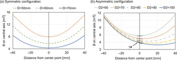
To analyze the induced electromagnetic field at the symmetric configuration, a parametric simulation is carried out at three different distances
 $D=D_1=D_2$
of 50, 60, and 70 mm. The obtained flux intensities
 $\vec{B}$
on the coaxis of the pair as function of the distance
 $D$
are plotted in Fig. 4(a). As can be seen, the resultant magnetic field is a superposition of the two magnetic fields arising from each electromagnet. It can also be observed that with an increment in the distance between the electromagnets, a decrement in the gradient near the center point is accompanied by a decrement in the intensity of the magnetic field. It can also be noted that it is not possible to obtain a perfect zero gradient region with the proposed configuration as any other coil pair setup. Therefore, a low gradient region is assumed to be a homogeneous field region if the induced force due to the gradient at any point of this region is lower than the friction force acting on the microrobot. From the aspect of homogeneity, if we consider the maximum accepted deviation in the gradient on the central line to be 5%, the width of the corresponding homogeneous line segments on the axis is measured as 16.4, 17.6, and 20.1 mm at the symmetric configuration for
 $D_1=D_2=D$
equals to 50, 60, and 70 mm, respectively. The results also show that this quasi-homogeneous region at the center can be widened by increasing the distance
 $D$
. Furthermore, it can be realized that the symmetric configuration can be used as an alternative to Helmholtz Coil due to its advantage of increasing the intensity of magnetic field and having an adjustable workspace.
Magnetic flux density on central axis in (a) symmetric configuration and (b) asymmetric configuration at different distances.

3.1.2. Asymmetric configuration
A similar parametric analysis is performed for the asymmetric configuration. The distances from the center point to each electromagnet are defined as
 $D_1=D$
and
 $D_2=D+\epsilon$
. The distance
 $D$
is set to 60 mm, and the asymmetry parameter (
 $\epsilon$
) is set to 0, 10, 20, 30, and 40 mm (
 $D_2=$
60, 70, 80, 90, 100 mm, respectively). The obtained intensity of the magnetic field
 $\vec{B}$
on the central axis is given as a function of the distances, as shown in Fig. 4(b). As it can be realized, the form of the field varies with the asymmetric positioning of the electromagnets (
 $\epsilon$
) when it is compared to the symmetric case. Moreover, the point at which the minimum magnetic field intensity occurred is shifting toward the farther electromagnet. Hence, it can be stated that the asymmetric placement of the electromagnets can be used to create a magnetic field gradient similar to Maxwell coil in any predefined region.
Furthermore, the two previous simulations’ results confirm that by using this re-configurable coaxial electromagnets set, the magnitude and gradient of the magnetic field can be modified purposefully. Namely, the proposed setup has the capability to create a combined effect of Maxwell and Helmholtz coils.
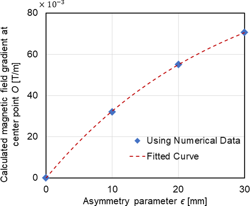
Magnetic field gradient at center point
 $G_u(\epsilon )$
with respect to asymmetry parameter
 $\epsilon$
(numerical results).

3.2. Relationship between the asymmetry parameter and the magnitude of magnetic force
The slope of the axial magnetic field gradient (
 $\frac{\partial B}{\partial u}$
) at the center point
 $O$
in Fig. 4(b) increases while the pair of electromagnets transforms from symmetrical to asymmetrical configuration (with
 $\epsilon$
). In order to formulate the relationship between these two variables,
 $\frac{\partial B}{\partial u}$
at
 $O$
is calculated by numerical derivation, and the results are given in Fig. 5 as a function of
 $\epsilon$
. It should be emphasized here that because the magnetic propulsion at the micro-scale is considered in this study, the center point
 $O$
was taken as the point of interest since it is considered as the position of the microrobot whose dimensions are assumed to be as small as a point compared to the size of the electromagnets. The representative mathematical correlation is found by using exponential curve fitting as in Eq. (6) (
 $R^2=0.99$
).
 \begin{equation} G_o(\epsilon )=18.2(1-e^{-0.0368\epsilon }) \end{equation}
where
 $G_o(\epsilon )=\frac{dB(\epsilon )}{d_u}$
is the function of the normalized magnetic field gradient
 $\frac{\partial B}{\partial u}$
at the center point
 $O$
along
 $u$
axis based on
 $B_o$
(5.8 mT in Fig. 4). The volume
 $V$
and the magnetization vector
 $\vec{M}$
can be expressed with a structural constant
 $C_\mu =V|\vec{M}|$
since they are characteristic properties of the permanent magnet of the microrobot. Consequently, the force equation can be rewritten in a simplified form as in Eq. (7).
 \begin{equation} \vec{F}=C_{\mu } G_o(\epsilon ) \end{equation}
Equation (7) and Fig. 5 indicate that the magnitude of the magnetic force
 $\vec{F}$
is proportional to the magnetic field gradient
 $\frac{\partial B}{\partial u}$
which can be controlled by changing the asymmetry parameter
 $\epsilon$
. Hence, the asymmetry parameter
 $\epsilon$
can be defined as a control variable of the magnetic force magnitude.
4. Control System
4.1. Control strategy and task space control
The proposed strategy for the microrobot position control is to apply a programmed sequences of an oriented 3D force along a desired route. The initial requirement for this strategy is to locate the microrobot on the center point
 $O$
of the symmetric configuration when no current flows through the coils. When the control system is activated (so the electromagnets), the error between the current and the following position on the sequence is calculated by using feedback from the task space vision system. The system then generates a 3D magnetic force output. As the force is defined by its 3D direction and magnitude, the end effector orientation (i.e., coaxis) and the electromagnet asymmetric position
 $\epsilon$
are updated accordingly. The microrobot then moves and loses its initial position in the coordinate frame of the end effector toward the following position on the sequence. The robot arm moves continuously to compensate the deviation of the microrobot position in that coordinate frame. This compensation is repeated with coaxis orientation at 5 DOF until fulfilling the designed path.
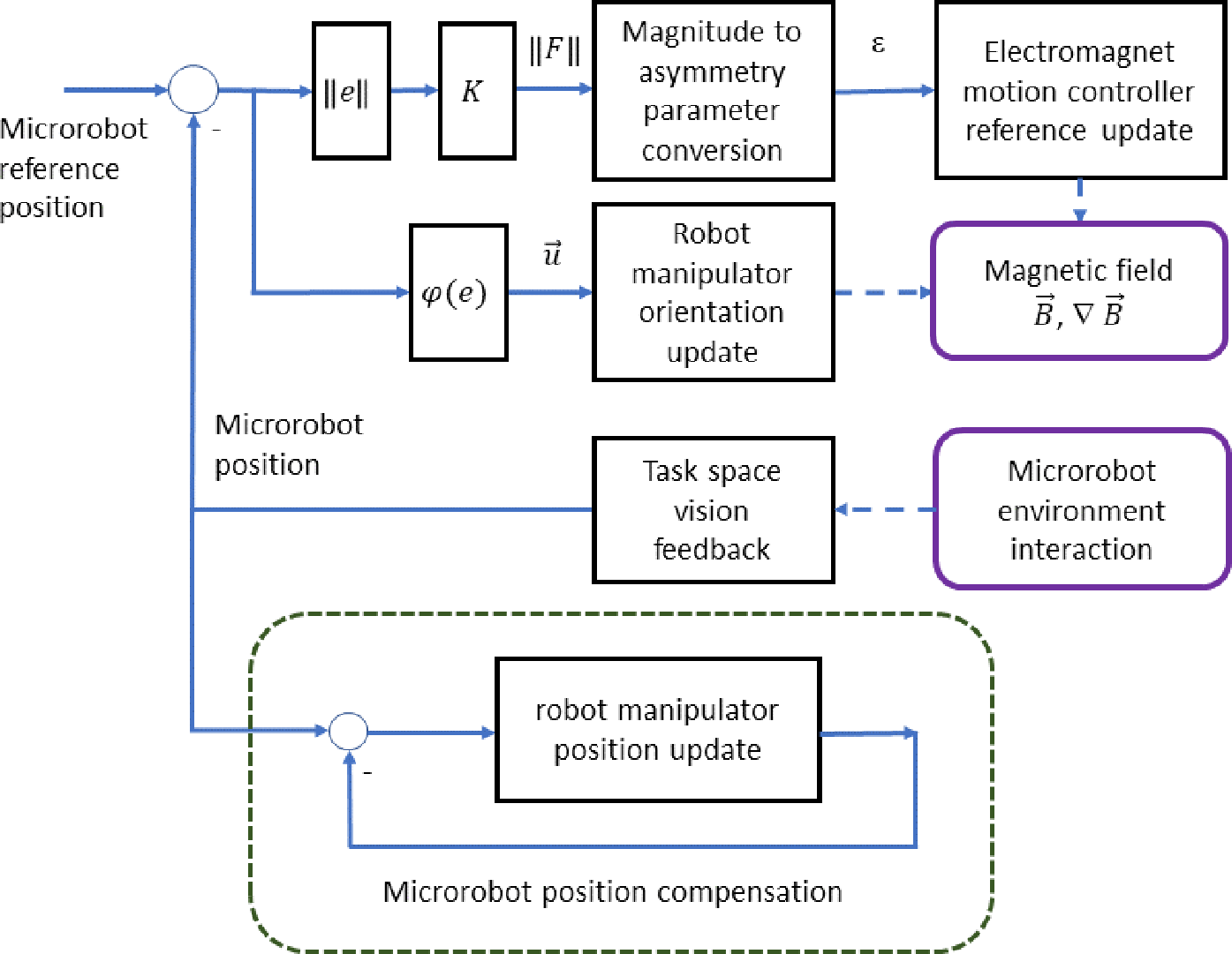
According to this strategy, the control problem of the proposed EMA system can be considered as a combination of a prime task and an auxiliary task, as shown in Fig. 6. The prime task objective is to compensate the position of the microrobot in the 3D workspace according to the programmed path, while the auxiliary task is to keep its position constant in the coordinate frame of the end effector (i.e, relative position to the electromagnets). Losing the defined relative position will shift the microrobot to another gradient region-namely, different magnitude of the magnetic force – which will cause losing control and sudden attraction of the microrobot to one of the electromagnets. To avoid that, the control system takes the actual position of the micro robot from the 3D vision setup and calculates the positioning error in the coordinate frame of the end effector. Afterward, the robot arm moves to compensate the relative positioning error. The speed of the relative compensation should be much faster than the motion of the microrobot to sustain the stability of the EMA system. The difference in operation speeds of the utilized robot arm controller (shown in a following section) guarantees that the microrobot positioning error with respect to the end effector is compensated approximately 20 times faster than microrobot positioning error in the task space.
Block diagram of the control system of the untethered EMA system.

Furthermore, proportional task space position controller is implemented to operate with the given position reference and the microrobot position feedback provided by the vision system. The positioning error is calculated in the 3D space as a vector with magnitude and orientation. The error magnitude is taken as a reference for the magnetic force magnitude controller. The magnetic force magnitude controller implements proportional control to calculate the required force magnitude by using the experimental relationship between
 $\nabla \vec{B}$
and the asymmetry parameter
 $\epsilon$
. The orientation error, on the other hand, is provided to the magnetic force orientation controller. The orientation controller updates the three DOF rotational references of the robot manipulator’s end effector. The combined effect of the magnetic force’s magnitude and orientation controller induces the task space force to compensate the microrobot positioning error according to the reference path. It is worthwhile to mention that controlling multiple microrobots within the ROI at the same time with the same strategy is possible if their magnetic fields are not interfering with each other. However, simultaneous independent multitask microrobot control is not achievable with the current EMA configuration.
4.2. Low-level controllers
As described above, the control of the electromagnet coaxial positions is necessary for setting the magnitude of the magnetic force. The translational motion of the electromagnets is provided by a timer belt mechanism that is driven by smart servo motors. Due to the usage of the servo motors, the mentioned control problem is solved by parameter tuning of an internal PI loop of the actuators. Furthermore, the real-time magnetic field control in this study does not involve any dynamical current updating. Therefore, the objective of the current control is to eliminate the steady-state error in the presence of disturbances. A custom PI controlled current driver is designed and implemented for this purpose [Reference Akcura, Alasli, Cetin and Tamer36].
4.3. Task space vision feedback system
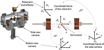
The feedback for the control is provided by a calibrated orthogonal stereo camera setup. The orthogonal setup consists of a static bottom view camera fixed under the test vessel and a side view camera fixed to the end effector (like an eye in hand configuration). The stereo reconstruction is carried out by taking homogeneous coordinate transformations that relate three frames: the end effector camera, bottom camera, and the side view camera, as illustrated in Fig. 7. The required input of the 3D position reconstruction is the position of the object in the image plane of both cameras. Consequently, the position of the microrobot should be tracked in an image flow during the actuation. The “boosting” algorithm is used for this purpose due to its applicability in real time tasks [Reference Grabner, Leistner and Bischof37]. The algorithm provides the position of a predefined rectangle in the image plane. Then, image segmentation routines and image moment calculations are carried out to define the necessary data of the image plane for the 3D reconstruction.
The used coordinate frames of the task space vision feedback system in stereo reconstruction.

5. Experimental Evaluation
In order to evaluate the performance of the proposed untethered actuation system and verify the numerical results of the analyzed electromagnetic field, a proof of concept actuator prototype is fabricated and a set of experiments are performed. The set of experiments are designed as follows:
The first set verifies the capability of the actuator prototype of inducing homogeneous magnetic fields and shifting toward magnetic field gradient according to the numerical results.
The second set first analyzes the performance of the actuator in inducing constant force and evaluates the time response parameter. In the second part, the transient force induction capability is analyzed and frequency response parameters are evaluated.
The third set demonstrates actuation of a microrobot model along a 3D helical route.
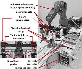
Actuator prototype.

5.1. Actuator prototype
The actuator prototype consists of a robotic arm, structural base of the EMA system, two coaxial electromagnets, electromagnet motion controller, electromagnet current controller, and task space feedback vision system, as shown in Fig. 8. Kuka Agilus KR6 R900 manipulator with positioning accuracy of 30
 $\mu$
m is used as the robotic arm. The structural base is a 3D printed bridge-like assembly made of ABS enforced with carbon fibers. The base holds the pair of electromagnets on two coaxial sliders and brass guide lines that align and allow the linear motion of them on the same axis. The electromagnets were fabricated according to an optimized design for the purpose of the proposed actuator. The design took into consideration the size constraints of the EMA system, which is set to 500 mm as the maximum total coaxial length limit including the total length of the electromagnets (300 mm) plus the maximum length of the ROI (200 mm), as discussed in details in Ref. [Reference Alasli, Çetin, Akçura, Kahveci, Can and Tamer35]. The electromagnet motion controllers control the position of each electromagnet with a motorized timer belt driven by Dynamixel XM430 Smart Servo motor. The servo motors have built-in functions for implementing different control routines; the PI controller mode is selected for this application. With this setup, the distance between the electromagnets can be arranged from 80 to 200 mm (D1 and D2: 40–100 mm). Furthermore, a positioning accuracy of 0.1 mm is achieved, and the system has a frequency of 16 Hz. The electromagnet current controllers are designed to eliminate steady state errors in presence of disturbances since the real time magnetic field control in this study does not involve any dynamical current updating. A PI controller is designed and implemented for this purpose with an observed bandwidth of 500 Hz. Two Basler cameras (with 16 mm lens and 1280 × 1800 image resolution at 25 Hz) providing planar position feedback with a resolution of 20
 $\mu$
m (at a fixed distance of 120 mm) is integrated to the system as the key-components of the task space feedback vision system. The proposed algorithm of the task space motion controller is coded on a single board computer NVIDIA Jetson TK1 and operated at 20 Hz.
5.2. Electromagnetic field experiments
To verify the capability of the actuator in generating homogeneous/gradient in the magnetic field at the symmetric/asymmetric configuration of electromagnets, the same conditions of the numerical analysis were applied. The magnitude of the magnetic field along the central line was measured by AFW Bell 5180 Gausmeter equipped with STD18-0404 probe at equal distances of
 $D_1=D_2$
50, 60, and 70 mm for the symmetric configuration at constant excitation current of 2 A. Afterward, the distance
 $D_1$
was kept constant at 60 mm, and
 $D_2$
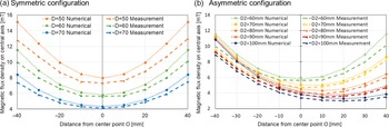
was shifted to 70, 80, 90, and 100 mm to observe the magnetic field gradient at the asymmetric configuration. The measured magnitude of the magnetic fields on the central line corresponding to the two configurations is plotted in Fig. 9.
Comparison between the experimental and numerical results of the magnetic field at (a) Symmetric configuration and (b) Asymmetric configuration.

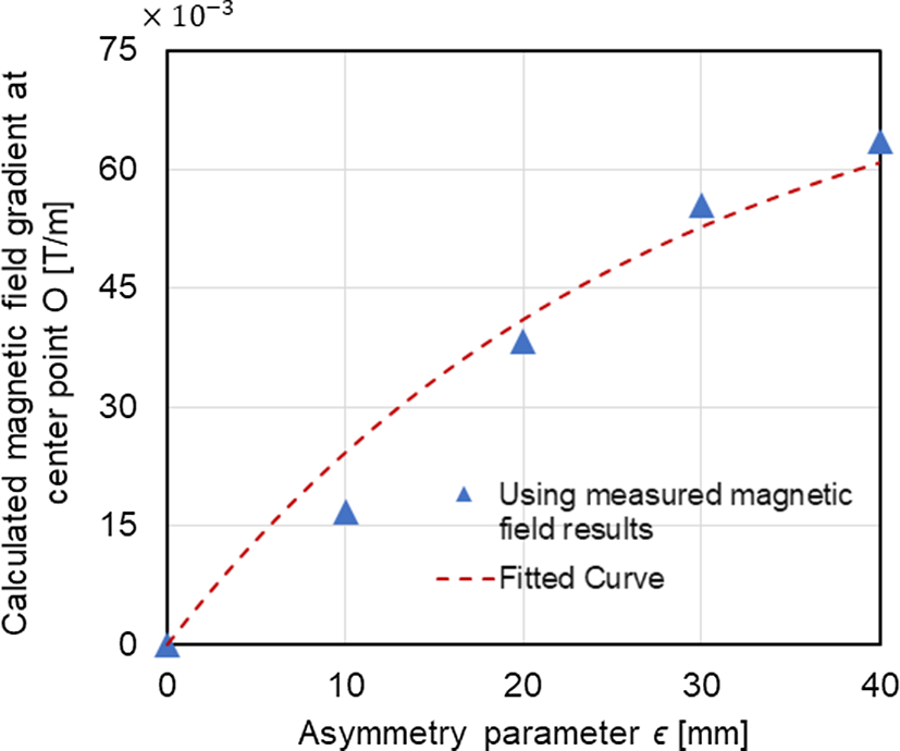
Magnetic field gradient at center point
 $G_u (\epsilon )$
with respect to asymmetry parameter
 $\epsilon$
(Experimental Results).

The experimental and numerical results around the center point
 $O$
(region of interest) are consistent, as can be observed from Fig. 9 for both the symmetric and asymmetric configurations. However, deviation increment is observed as the measurement point approaches the electromagnet. The deviation can be attributed to the losses caused by environmental conditions and the nonlinear effects arising from the core structure. Furthermore, the gradient at point
 $O$
can be calculated by using the results of Fig. 9(b). For that, a function
 $B(u)$
of the magnetic field magnitude on the central line was obtained as a polynomial regression at the second order for each
 $D_2$
. The gradient at point
 $O$
is then evaluated by taking the derivative of the polynomial at
 $O$
. The calculated values are given in Fig. 10 with respect to the asymmetry parameter (
 $\epsilon$
), which is 0, 10, 20, 30, and 40 mm for
 $D_2$
60, 70, 80, 90, and 100 mm, respectively. The representative mathematical relationship is found by employing exponential curve fitting as in Eq. (8) (
 $R^2=0.97$
).
 \begin{equation} G_u (\epsilon )=14.1\left(1-e^{(-0.366\epsilon )}\right) \end{equation}
By observing the fitted exponential curve in Fig. 10 and Eq. (8), it can be seen that it is in the form
 $K(1-e^{-\kappa \epsilon })$
, which is characterized by two parameters
 $\kappa$
and
 $K$
. The parameter
 $\kappa$
defines the spatial dependency of the function output on the asymmetry parameter
 $\epsilon$
, while K acts as a scaling factor. By comparing Eqs. (8) with (6) (of the numerical results), it can be noticed that
 $\kappa$
in both equations are close to each other (0.0366 in Eq. (6) and 0.0368 in Eq. (8)). The similarity in
 $\kappa$
indicates that the spatial dependency of the magnetic field gradient has same characteristics in both numerical and experimental studies. Furthermore, the scaling factors can be better compared when they are normalizing based on
 $B_o$
(5.8 and 5.6 mT for the numerical analysis [Fig. 4] and the experimental measurements [Fig. 9] values, respectively). The normalized
 $K$
in Eq. (8) (14.1) is smaller than the one in Eq. (6) (18.2) due to the weakening of the gradients with distance to pole’s face and the real world implementation.
5.3. Magnetic force experiments
A cylindrical magnet with a diameter of 1 mm and height of 1 mm is used as a microrobot prototype for this set of experiments. The remanence of the magnet is 1.28 mT, and the calculated magnetic dipole (
 $C\mu$
) value is
 $8.00\times 10^{-7} A.m^2$
. The microrobot motion is observed with the cameras, while it is moving in a fluid with a viscosity of 557 mPa.s inside the test vessel.
5.3.1. Constant force (gradient) experiments
As observed from Eq. (6), the relation between the magnetic field gradient
 $\nabla _u\vec{B}$
and the force acting on the magnetized part of the microrobot is proportional. Based on this, a set of experiments to analyze the microrobot motion under the effect of constant force were performed. The asymmetry parameter (
 $\epsilon$
) is changed from 10 to 40 mm with 10 mm steps at initial
 $D$
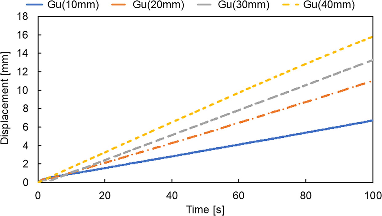
= 60 mm, while the relative distance of the microrobot to the electromagnets is kept constant. The experiments are carried out at open loop control and the force was applied for 100 s. The results of tracking the position of the microrobot with time at different
 $\epsilon$
are shown in Fig. 11. As it can be noticed from the slopes of the lines, the microrobot reaches a constant velocity at the steady state. Furthermore, increasing the gradient (
 $\epsilon$
) results in an increment in the steady-state velocity.
Motion of the microrobot under the effect of a constant force.

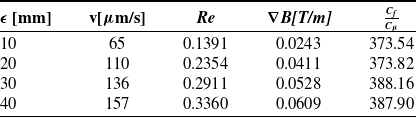
Physically, microrobot velocity reaches the steady state when the electromagnetic force is at equilibrium with the drag force by compensating the gravitational force with buoyancy force and neglecting the lift force since the microrobot is considered perfectly symmetric. By exploiting this principle, the capability of the proposed actuator of manipulating microrobot at constant force can be evaluated. The steady state velocity and the Reynolds number for each experiment are first calculated and given in Table I. Since the Reynolds numbers are smaller than 1, drag force model (given in Eq. (9)) is applied according to Stokes’ law.
 \begin{equation} F_c=C_f.v \end{equation}
where
 $C_f$
is the drag coefficient that depends on the geometry of the microrobot and the viscosity of the fluid and
 $v$
is the measured velocity of the microrobot. By applying Newton’s second law, the equation of the motion can be written as in Eq. (10).
 \begin{equation} m\dot{v}=C_\mu G_u(\epsilon )-C_f.v \end{equation}
At steady state, the time derivative term is zero and a proportional relationship between the velocity and the magnetic gradient is obtained as a constant ratio
 $\frac{C_\mu }{C_f}$
, which is defined only by the characteristics of the fluid and microrobot. Since the experiments are performed with the same fluid and same microrobot, the ratio
 $\frac{C_\mu }{C_f}$
should be constant. Consequently, the actuator capability of controlling the force magnitude can be evaluated by calculating this ratio for each
 $\epsilon$
, as given in Table I. Based on the experimental results, the average of the ratios is 380.8
 $\frac{mT.s}{mm^2}$
with standard deviation of 7.2
 $\frac{mT.s}{mm^2}$
. Since the standard deviation corresponds to 2% of the average, the ratios are assumed to be constant, and it can be said that it is possible to sustain constant magnitude of the induced force during actuation via the proposed actuator.
Experimental results and calculated parameters of the constant force experiments.

5.3.2. Transient force (gradient) experiments
The capability of generating transient force is tested with sinusoidal force (gradient). To apply a sinusoidal gradient on the microrobot at
 $O$
of the form
 $G_u(t)=|G_u(t)|sin(2\pi ft)$
, the asymmetry parameter (
 $\epsilon$
) should be given as a generic sine wave input to the motion controller of the electromagnets. For that, the time dependent form of
 $\epsilon$
, Eq. (11), was first obtained from the inverse of the experimental-based
 $G_u(t)$
function (Eq. (7)).
 $\epsilon (t)$
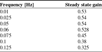
data according to the frequency was then generated and fed to the two smart servo motors who drive the coaxial electromagnets. The applied frequency was changed from 0.01 to 0.125 Hz, while its amplitude is kept constant at 0.025 T/m. The duration of each experiment is set to 6 times the period of the input. The last three oscillations were taken to ensure analysis at the steady state.
 \begin{equation} \epsilon (t)=-\frac{1}{0.366}\frac{log(1-G_u (t))}{14.1} \end{equation}
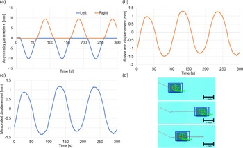
Figure 12 presents the microrobot responsive motion, the actuator commands to the left and right motors of the electromagnets, and the motion of the end effector of the robotic manipulator at a 0.01 Hz sinusoidal input. As expected, the microrobot makes steady state simple harmonic motion on the central line under the effect of the sinusoidal force. Furthermore, the synchronized motion of the end effector for compensating the microrobot motion in order to keep it at the center point (i.e., constant
 $\nabla \vec{B}$
) can be also realized.
Steady state gain with respect to frequency.

Table II summarizes the obtained results of the sinusoidal magnetic gradient (force) experiments. The results present the frequency dependent change in the steady state gains. The gain is calculated as the ratio of the sinusoidal steady state microrobot velocity magnitude (output) to the sinusoidal gradient magnitude (input). The gains can be considered as a representative value of the mechanical admittance (
 $v/F$
) for the interaction between the actuator and microrobot since the magnetic force is proportional to the magnetic field gradient. The results also reveals that the bandwidth of the experimental actuator is 0.1 Hz.
5.4. 3D motion demonstration
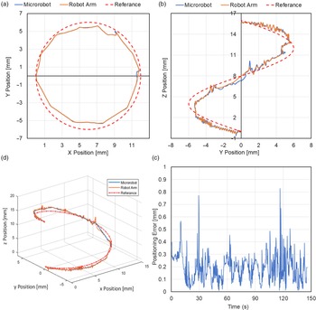
Manipulation of a microrobot model on a helical route is demonstrated in Fig. 13 and the supplemental video. At initial stage, the programmed path is uploaded to the space task controller. The microrobot model is placed at the central point with respect to the robot arm and both cameras are activated to log the position of microrobot as the central position. Then, the electromagnetic actuator is activated and a magnetic force is applied on the microrobot. At the proceeding time instant, the control system receives the position of the microrobot while its moving from the cameras and calculates its displacement error with respect to the central position on the image plane. According to the programmed path, the space task controller applies proportional control to give an incremental position and direction command to the robot arm by scaling the observed motion in the image plane to the real world coordinates in order to compensate the displacement error. The last loop is repeated until the microrobot fulfils the whole path. Figure 13 presents the tracks of the microrobot, robot arm on XY plane (bottom camera), YZ plane (frontal camera) and the stereo reconstruction 3D image by the space task vision system according to the reference path. Moreover, the average of the absolute error according to the nearest point on the reference path and the standard deviation
 $\sigma$
are 190 and 101
 $\mu$
m, respectively, as it can also be realized from the graphs. It is worth mentioning here that a part of the error is related with the robotic arm and image noise (see the supplemental video).
Frequency response of the actuator (Magnetic gradient vs microrobot velocity).

The tracks of the microrobot and the robot arm on (a) XY plane (bottom camera), (b) YZ plane (frontal camera), (c) the stereo reconstructed 3D path and (e) the absolute error according to the nearest point on the helical reference path.

The performance of the proposed system is comparable with other EMA systems in terms of positioning accuracy and velocity (Table I). For instance, the stationary EMA system, developed by Khalil et al., propelled a sperm-cell shaped microrobot at low magnetic field strength of 1.39 mT at an average velocity of 25
 $\pm$
10
 $\mu$
m/s with an accuracy of 90
 $\pm$
40
 $\mu$
m [Reference Khalil, Magdanz and Sanchez38]. Similar stationary systems also reported positioning errors of 100
 $\mu$
m at 122
 $\mu$
m/s for microsphere robot (r = 350
 $\mu$
m) [Reference Ongaro, Pane, Scheggi and Misra3] and 310
 $\mu$
m for 400–4000
 $\mu$
m multi-microrobots [Reference Diller, Giltinan and Sitti39]. On the other hand, mobile EMA systems such as the ARMM system of Heunis et al. [Reference Heunis, Wotte, Sikorski, Furtado and Misra40], positioned a magnetic endovascular catheter at an accuracy of 2.09
 $\pm$
0.49 mm. Moreover, it is worth mentioning here the conclusion of Franz et al. of their comprehensive review of electromagnetic tracking systems in medicine. They stated that electromagnetic steering systems have an average accuracy of 1 mm in minimal interference environments. Nevertheless, any source of distortion can cause drastic accuracy drops [Reference Franz, Haidegger, Birkfellner, Cleary, Peters and Maier-Hein41].
6. Conclusion
In summary, this study developed a novel electromagnetic actuation system for microrobotic manupulation. In this system, a pair of coaxial electromagnets were exploited as a source and for forming the magnetic field by symmetrical/asymmetrical pair positioning. The homogeneous/gradient (symmetrical/asymmetrical configuration) magnetic field forms were analyzed numerically and verified experimentally. An exponential relationship between the gradient magnitude and the asymmetry parameter
 $\epsilon$
was observed. By using this relationship, the magnitude of the induced force was controlled. Furthermore, forces on the microrobot were evaluated experimentally at the steady and the transient states. Microrobot manipulation on a helical route was demonstrated with transporting the magnetic field in 3D with 5 DOF by the aid of robotic manipulator and closed loop control system with integrated vision feedback system. The absolute error mean from the reference path was realized to be 191
 $\mu$
m with
 $\sigma$
= 101
 $\mu$
m, which is comparable with the positioning error of other EMA systems. Future works are recommended to develop the proposed EMA system for the purpose of nanoscale manipulation. Subsequent works for developing the feedback method for opaque ROI by utilizing ultrasound, radio frequencies, positron emitting marking, or any similar techniques are also of great importance for medical application such as microsurgery and drug delivery.
Financial Support
This work was supported by the Scientific and Technological Research Council of Turkey (TUBITAK, project No. 215M879)
Conflicts of Interest
The authors declare no conflict of interest regarding this research paper with any person or organization.
Ethical Considerations
The authors declare none.
Authors’ Contributions
The contributions of the authors are as follows, Levent Çetin: Conceptualization of the study, methodology, and experiment design. Abdulkareem Alasli: Mechanical design, data curation, and original draft preparation. Nail Akçura: Experiments, data curation, and electrical and mechanical design. Aytaç Kahveci: Experiments, data curation, and computer programming. Fatih Cemal Can: Mechanical design. Özgür Tamer: Electromagnetic design and original draft preparation.
Supplementary Material
To view supplementary material for this article, please visit https://doi.org/10.1017/S0263574722000418.