1. Introduction
The breaking of ocean surface gravity waves figures in a number of different environmental processes including air–sea exchange of heat, momentum and energy, underwater optics and acoustics, and upper ocean mixing (Melville Reference Melville1996). During active breaking, the process may be characterized as a two-phase turbulent flow with a complex interface, involving a wide range of temporal and spatial scales. For practical use in large-scale wave modelling, the onset of breaking and subsequent integral measures of the process, such as total loss of wave energy and momentum flux, need to be parameterized using available pre-breaking information.
For many decades, considerable attention has been paid to find a robust and universal methodology to predict the onset of steepness-limited unsteady breaking waves (Song & Banner Reference Song and Banner2002; Wu & Nepf Reference Wu and Nepf2002; Banner & Peirson Reference Banner and Peirson2007; Tian, Perlin & Choi Reference Tian, Perlin and Choi2008). There are several important reviews on the topic of wave breaking (Banner & Peregrine Reference Banner and Peregrine1993; Melville Reference Melville1996; Duncan Reference Duncan2001; Kiger & Duncan Reference Kiger and Duncan2012). Recently, Perlin, Choi & Tian (Reference Perlin, Choi and Tian2013) have reviewed the latest progress on prediction of geometry, breaking onset and energy dissipation of intermediate- and deep-water breaking waves. The predictive parameters involved can be categorized as (i) geometric, (ii) kinematic, and (iii) dynamic criteria. As summarized in Perlin et al. (Reference Perlin, Choi and Tian2013, § 3), one of the most reliable criteria which can distinguish between breaking packets from those that do not break is the dynamic criterion proposed by Song & Banner (Reference Song and Banner2002). They proposed a dimensionless parameter,
 ${\it\delta}(t)$
, to measure the growth rate of the local wave energy density, given by
 $$\begin{eqnarray}{\it\delta}(t)=\frac{1}{{\it\omega}_{c}}\frac{\text{D}\langle {\it\mu}\rangle }{\text{D}t},\quad {\it\mu}=\frac{E_{max}k^{2}}{{\it\rho}^{l}g},\end{eqnarray}$$
where
 ${\it\omega}_{c}=2{\rm\pi}f_{c}$
is a characteristic angular frequency (e.g. taken as the initial angular frequency of the centre component of the dispersive packet),
 $\text{D}/\text{D}t$
represents the total derivative following the wave group,
 ${\it\mu}$
is the dimensionless local wave energy density,
 $E_{max}$
is the maximum local wave energy density given in § 3,
 $k$
is the local wavenumber,
 ${\it\rho}^{l}$
is the liquid density and
 $g$
is the gravitational acceleration. Here, the averaging procedure denoted by
 $\langle \;\rangle$
was proposed by Song & Banner (Reference Song and Banner2002) to remove the large oscillation of
 ${\it\mu}$
, involving the determination of the upper and lower envelopes of
 ${\it\mu}$
as described in Song & Banner (Reference Song and Banner2002, appendix B). Song & Banner (Reference Song and Banner2002) found that this dynamically based mean growth rate of the local energy density maximum along a wave packet had a common threshold value of
 $[1.4\pm 0.1]\times 10^{-3}$
associated with the initiation of breaking. As pointed out by Perlin et al. (Reference Perlin, Choi and Tian2013), the calculation of the time-averaged local wave energy density
 $\langle {\it\mu}\rangle$
is non-trivial, and, thus, the application of the criterion, e.g. in phase-resolving nonlinear wave prediction models, may be limited. A modified version of (1.1), which removes the required post-processing procedure in the calculation of
 $\langle {\it\mu}\rangle$
, is defined in § 3 and is tested for the packets considered here.
In addition to a selected pre-breaking diagnostic parameter, the accurate estimation of total loss of wave energy and momentum flux are needed to find a robust parameterization for the breaking strength, e.g. the averaged breaking-induced wave energy dissipation rate. During the last three decades, laboratory experiments have been conducted for the estimation and parameterization of total energy and momentum flux losses and their rates (Duncan Reference Duncan1983; Rapp & Melville Reference Rapp and Melville1990; Banner & Peirson Reference Banner and Peirson2007; Drazen, Melville & Lenain Reference Drazen, Melville and Lenain2008; Tian, Perlin & Choi Reference Tian, Perlin and Choi2010, Reference Tian, Perlin and Choi2012). The most up-to-date review may be found in Perlin et al. (Reference Perlin, Choi and Tian2013, § 4). Inherent difficulties associated with the measurement of an instantaneous velocity field during an active breaking event make direct estimates of energy and momentum flux in a breaking region impractical. The common practice is to approximate energy and momentum flux through surface elevation measurements taken at fixed locations upstream and downstream of a break point, using a wave theory (usually linear theory) and a simple control volume analysis to obtain estimates of total fluxes (e.g. see Rapp & Melville Reference Rapp and Melville1990, § 2.4).
Because numerical computations based strictly on inviscid, irrotational flow theory cannot proceed beyond the onset stage of breaking, a post-breaking flow field becomes unavailable. As summarized by Perlin et al. (Reference Perlin, Choi and Tian2013, § 6), most two-phase viscous numerical simulations for steepness-limited breaking waves are limited to the evolution of a periodic unstable wave train having relatively low Reynolds numbers (
 ${\sim}10^{4}$
) and short wavelengths (
 ${<}$
0.3 m). An exception is noted in recent work by Derakhti & Kirby (Reference Derakhti and Kirby2014a
). Examining bubble entrainment and turbulence modulation by dispersed bubbles in isolated unsteady breaking waves generated by dispersive focusing (with the same scale as in the previous laboratory experiments), they used an Eulerian–Eulerian polydisperse two-fluid model to performed large-eddy simulation (LES), together with a dynamic Smagorinsky sub-grid formulation for turbulence closure. As opposed to direct numerical simulations, the dissipative scales of the process as well as liquid–bubble interaction were sub-grid scale and were modelled using the available closure models, which is an inherent limitation in any LES study.
In this paper, we present direct estimates of total energy and momentum flux in unforced intermediate- and deep-water unsteady breaking waves generated by dispersive focusing. Both spilling and plunging breaking packets are considered. The accuracy of estimating these integral measures based on free surface measurements and using a characteristic wave group velocity is examined in detail. In addition, we examine nonlinear interactions of different frequency components in a focused wave packet as well as interaction effects on a characteristic wave group velocity both in non-breaking and breaking packets. Phase locking between spectral components is observed in the breaking region as well, and subsequently illustrated by calculating the wavelet bispectrum.
Beside dispersive energy focusing, other mechanisms such as modulational instability (Benjamin & Feir Reference Benjamin and Feir1967; Melville Reference Melville1982) and wind forcing (Grare et al.
Reference Grare, Peirson, Branger, Walker, Giovanangeli and Makin2013; Schwendeman, Thomson & Gemmrich Reference Schwendeman, Thomson and Gemmrich2014) can induce wave breaking. Although some of the available estimates of the non-dimensional breaking strength parameter,
 $b$
, in the field (Thomson, Gemmrich & Jessup Reference Thomson, Gemmrich and Jessup2009; Schwendeman et al.
Reference Schwendeman, Thomson and Gemmrich2014) are comparable to those in spillers due to dispersive energy focusing (Drazen et al.
Reference Drazen, Melville and Lenain2008; Tian et al.
Reference Tian, Perlin and Choi2010), most of the field estimations of
 $b$
(Phillips, Posner & Hansen Reference Phillips, Posner and Hansen2001; Gemmrich, Banner & Garrett Reference Gemmrich, Banner and Garrett2008; Gemmrich et al.
Reference Gemmrich, Zappa, Banner and Morison2013) tend to be more consistent with the observed
 $b$
values in weak spillers due to modulational instability (Banner & Peirson Reference Banner and Peirson2007; Allis Reference Allis2013). Here, we briefly establish that the present model is capable of capturing breaking waves due to modulational instability. A more detailed evaluation of this class of weak breaking events will appear in a separate paper.
In § 2, the model set-up and choice of experimental data are explained. Results for breaking-onset prediction, energy and momentum flux are presented in §§ 3–5, respectively. Conclusions are given in § 6.
2. Model set-up and choice of experimental conditions
A detailed description of the polydisperse two-fluid model used here as well as boundary conditions may be found in Derakhti & Kirby (Reference Derakhti and Kirby2014a , § 2). Here, the incident wave boundary condition and model set-up are discussed briefly.
All model simulations are performed with the model initialized with quiescent conditions. An incident wave packet is then generated at the model upstream boundary. The input wave packet was composed of
 $N$
sinusoidal components of steepness
 $a_{i}k_{i},i=1,\ldots ,N$
where
 $a_{i}$
and
 $k_{i}$
are the amplitude and wavenumber of the
 $i$
th frequency component. Based on linear superposition and by imposing that the maximum
 ${\it\eta}$
occurs at
 $x_{b}$
and
 $t_{b}$
, the total surface displacement at the incident wave boundary
 $x=0$
is given by
 $$\begin{eqnarray}{\it\eta}(0,t)=\mathop{\sum }_{i=1}^{N}a_{i}\cos [2{\rm\pi}f_{i}(t-t_{b})+k_{i}x_{b}],\end{eqnarray}$$
where
 $f_{i}$
is the frequency of the
 $i$
th component, and
 $x_{b}$
and
 $t_{b}$
are the predefined, linear theory estimates of location and time of breaking, respectively (e.g. see Rapp & Melville Reference Rapp and Melville1990, § 2.3). The discrete frequencies
 $f_{i}$
were uniformly spaced over the band
 ${\rm\Delta}f=f_{N}-f_{1}$
with a central frequency defined by
 $f_{c}=1/2(\,f_{N}+f_{1})$
. Different theoretical global steepness,
 $S=\sum _{i=1}^{N}a_{i}k_{i}$
, and bandwidth,
 ${\rm\Delta}f/f_{c}$
, lead to spilling or plunging breaking, where increasing
 $S$
and/or decreasing
 ${\rm\Delta}f/f_{c}$
increases the breaking intensity (see Drazen et al. (Reference Drazen, Melville and Lenain2008) for more details). Free surface displacements and velocities for each component are calculated using linear theory and then superimposed at
 $x=0$
.
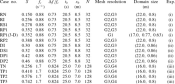
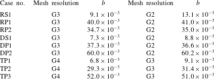
The input packet parameters as well as mesh resolutions and domain sizes for cases considered here are summarized in table 1. The convergence study may be found in Derakhti & Kirby (Reference Derakhti and Kirby2014b ). The model parameters for a polydisperse bubble phase are chosen as summarized in Derakhti & Kirby (Reference Derakhti and Kirby2014a , table 4).
Input parameters for the 2-D and 3-D simulated cases. (i) Rapp & Melville (Reference Rapp and Melville1990),
 $d=0.6$
m,
 $d/L_{c}=0.3$
intermediate depth, constant-amplitude packets; (ii) Drazen et al. (Reference Drazen, Melville and Lenain2008),
 $d=0.6$
m,
 $d/L_{c}=0.3$
intermediate depth, constant-steepness packets; (iii) Tian et al. (Reference Tian, Perlin and Choi2012),
 $d=0.62$
m,
 $d/L_{c}=1.1$
deep water, constant-steepness packets. Here,
 $d$
is the still water depth,
 $L_{c}$
is the wavelength of the centre frequency component of the incident packet
 $f_{c}$
,
 $S$
is the theoretical linear global wave steepness,
 ${\rm\Delta}f$
is the packet band width,
 $x_{b}$
and
 $t_{b}$
are the predefined, linear theory estimates of location and time of breaking, respectively and
 $N$
is the number of different wave components in the packet. In constant-steepness packets, each wave component has a different amplitude,
 $a_{i}=S/(k_{i}N)$
such that component steepness
 $a_{i}k_{i}$
is constant with respect to
 $i$
. In constant-amplitude packets, on the other hand, all the components have the same amplitude,
 $a_{i}=a$
. Rapp & Melville (Reference Rapp and Melville1990) defined the global steepness of a constant-amplitude packet as
 $S=k_{c}\sum _{i=1}^{N}a_{i}=k_{c}Na$
and, thus,
 $a=S/(k_{c}N)$
. Different mesh grid densities are:
 $\text{G1}=$
(
 ${\rm\Delta}x=21.5$
,
 ${\rm\Delta}y=7.0,{\rm\Delta}z=7.0$
) mm,
 $\text{G2}=({\rm\Delta}x=18.3,{\rm\Delta}z=5.0)$
mm,
 $\text{G3}=({\rm\Delta}x=10.0,{\rm\Delta}z=5.0)$
mm, and
 $\text{G4}=({\rm\Delta}x=5.0,{\rm\Delta}z=5.0)$
mm.

For non-breaking cases,
 $t_{b}$
and
 $x_{b}$
are used as the reference for the time and
 $x$
direction respectively. For breaking packets, the references for time and
 $x$
direction are
 $t_{ob}$
and
 $x_{ob}$
, respectively. For plunging breakers,
 $t_{ob}$
and
 $x_{ob}$
are the time and location at which the falling jet hits the undisturbed forward face of the wave. For spilling breakers, on the other hand,
 $t_{ob}$
and
 $x_{ob}$
are the time and location at which a vertical tangent develops near the wave crest. Normalized horizontal position and time can then be written as
 $$\begin{eqnarray}x^{\ast }=\frac{x-x_{ob}}{L_{s0}},\quad t^{\ast }=\frac{t-t_{ob}}{T_{s0}},\end{eqnarray}$$
where
 $L_{s0}$
and
 $T_{s0}$
are the characteristic length and time scales of the carrier wave in the packet far upstream of the focal/break point, and are calculated based on the spectrally weighted frequency of the wave packet
 $f_{s}$
given by
 $$\begin{eqnarray}f_{s}=\frac{\displaystyle \sum f_{i}|\mathscr{F}_{i}|^{2}{\rm\Delta}f_{i}}{\displaystyle \sum |\mathscr{F}_{i}|^{2}{\rm\Delta}f_{i}},\end{eqnarray}$$
where,
 $\mathscr{F}_{i}$
and
 $f_{i}$
are the discrete Fourier transform and the frequency of the
 $i$
th component of the wave train, respectively.
 ${\rm\Delta}f_{i}$
is the frequency difference between components, which is constant here. The characteristic wavelength
 $L_{s}$
and period
 $T_{s}$
, hereafter called spectrally weighted wavelength and period, are calculated based on
 $f_{s}$
and using the linear dispersion relation. Tian et al. (Reference Tian, Perlin and Choi2010) found that this choice of the characteristic wave parameters provided the best data collapse for their wave packets. We also found that the corresponding length and time scales of the carrier wave in the packet close to the focal/break point are predicted more accurately by this choice of the characteristic parameters compared with those of the centre frequency of the wave packet, especially for our deep-water packets. For constant-amplitude packets we have
 $f_{s0}\approx f_{c}$
, and thus
 $L_{s0}\approx L_{c}$
and
 $T_{s0}\approx T_{c}$
, where subscript
 $c$
indicates the centre frequency component of the wave packet.
Definitions of the local wave parameters.
 $k$
and
 $a$
are the local wavenumber and amplitude respectively. The wave propagates from the left to the right.

Temporal variations of (a,c,e) the normalized local energy density maximum,
 ${\it\mu}$
, and (b,d,f) its normalized growth rate,
 ${\it\xi}$
, for different breaking and non-breaking packets. (a,b) Intermediate-depth incipient breaking RI (– – –), spilling breaker RS1 (— ⋅ —), plunging breaker RP1 (——); (c,d) intermediate-depth incipient breaking DI (
 $\cdots \cdots$
), spilling breaker DS1 (– – –), plunging breaker DP1 (— ⋅ —), plunging breaker DP2 (——); and (e,f) deep-water non-breaking packet TN (
 $\cdots \cdots$
), weak plunging breaker TP1 (– – –), plunging breaker TP2 (— ⋅ —), plunging breaker TP3 (——). Horizontal lines show
 ${\it\mu}=0.2$
and
 ${\it\xi}=0.05$
. Thick lines in (a,b) are the results for RP1(3-D).

Temporal variations of the ratio of the potential energy density to the total energy density for (a) RI, (c) RS1, (e) RP1, (b) TN, (d) TP2, ( f) TP3; at the locations of
 $E_{max}$
(


3. Prediction of the onset of wave breaking
Avoiding the post-processing procedure in (1.1), we define the normalized growth rate of the time-dependent
 ${\it\mu}=E_{max}k^{2}/{\it\rho}^{l}g$
as
 $$\begin{eqnarray}{\it\xi}(t)=\frac{1}{{\it\omega}_{s0}}\frac{\text{D}{\it\mu}}{\text{D}t},\end{eqnarray}$$
where
 ${\it\omega}_{s0}=2{\rm\pi}f_{s0}$
is the pre-breaking characteristic wave angular frequency, and
 $k$
is the local wavenumber calculated based on two consecutive zero-crossings adjacent to the breaking crest (see figure 1) as suggested by Tian et al. (Reference Tian, Perlin and Choi2008). Here,
 $E_{max}$
is the time-dependent, non-horizontally averaged local maximum of the ensemble-averaged depth-integrated total energy density
 $E(t,x)$
along the wave group given by
 $$\begin{eqnarray}E(t,x)=\left\langle \int _{-d}^{{\it\eta}}\frac{1}{2}{\it\rho}u_{i}^{2}\,\text{d}z\right\rangle +\left\langle \int _{-d}^{{\it\eta}}{\it\rho}gz\,\text{d}z\right\rangle +\frac{1}{2}{\it\rho}^{l}gd^{2}=E_{k}+E_{p},\end{eqnarray}$$
where
 $i=1,2,3$
refers to the
 $x,y$
and
 $z$
directions respectively;
 ${\it\rho}={\it\alpha}{\it\rho}^{l}$
is the mixture density, and
 ${\it\alpha}$
is liquid volume fraction;
 $d$
is the still water depth,
 $z$
is the vertical distance to the still water level (positive upward),
 $E_{k}$
is the ensemble-averaged depth-integrated kinetic energy density and
 $E_{p}$
is the ensemble-averaged depth-integrated potential energy density. Hereafter,
 $\langle \cdot \rangle$
indicates ensemble averaging and is approximated by spanwise averaging as in Derakhti & Kirby (Reference Derakhti and Kirby2014a
, § 2.8). No spatial averaging is employed in the 2-D simulations.
Figure 2 shows that, in all the intermediate- and deep-water breaking packets considered here, the corresponding values of
 ${\it\xi}$
before breaking, say
 $-0.5<t^{\ast }$
, exceed an approximate threshold value of
 ${\it\xi}_{th}=0.05$
. In the incipient breaking packets RI and DI, it is seen that
 ${\it\xi}_{max}\sim 0.05$
, also supporting the selection of
 ${\it\xi}_{th}=0.05$
as a maximum normalized growth rate of the local wave energy density maximum for the non-breaking packets. The exceedance of the threshold value
 ${\it\xi}_{th}=0.05$
at
 $t^{\ast }\approx -1.5$
for the deep-water packet with multiple plungers TP3 is because of the preceding weaker breaking wave in the packet before the main breaker at
 $t^{\ast }=0$
, observed both in the simulation and the corresponding measurement by Tian et al. (Reference Tian, Perlin and Choi2012). Thus, the criterion is capable of detecting multiple breaking events in a wave group. Figure 2 also shows that
 ${\it\mu}>0.2$
at which
 ${\it\xi}>{\it\xi}_{th}$
in all breaking packets except the deep-water weak plunging breaker TP1. For the intermediate-depth plunging breaking case RP1, comparing the results of the 2-D and the 3-D simulations, shown in (b) with thin and thick solid lines respectively, we may conclude that the 2-D simulation captures the evolution of
 ${\it\xi}$
fairly accurately.
The evaluation of
 $E_{max}$
needs the spatio-temporal variation of both the free surface and velocity field. Although the free surface locations are easy to measure, the velocity field may not be available especially in in-situ measurements. Thus, the estimation of
 $E_{max}$
based only on the free surface information is of potential interest. Figure 3 shows that the location of
 $E_{max}$
switches between the crest maxima and trough maxima before and after the focal/break point both in the intermediate- and deep-water packets. However, it is always on the crest maxima close to the focal/break point, say
 $-1<t^{\ast }<0$
, at which
 ${\it\xi}$
goes beyond the threshold value of 0.05. As
 $S$
increases, the location of
 $E_{max}$
occurs at the crest maxima more frequently. In addition, increasing
 $S$
results in decreasing the
 $E_{p}/E$
ratio at the crest maxima and in increasing the
 $E_{p}/E$
ratio at trough maxima; a similar trend can be seen in Tian et al. (Reference Tian, Perlin and Choi2008, figure 11). Thus, we may estimate
 $E_{max}\approx E_{p}^{cm}/{\it\lambda}$
before the break point, where
 $E_{p}^{cm}=({\it\rho}^{l}gz_{max}^{2})/2$
is the local potential energy density at the crest maxima and
 ${\it\lambda}=E_{p}/E_{max}$
, shown by thick solid lines in figure 3, varies from
 ${\approx}$
0.6 for
 $t^{\ast }<-1$
down to
 ${\approx}$
0.5 at breaking-onset.
4. Fractional and total losses of energy flux
The ensemble- and time-averaged depth-integrated horizontal energy flux of a 2-D wave packet per unit crest length over the time
 $t=t_{1}\rightarrow t_{2}$
,
 $\overline{\overline{F^{E}}}$
, can be written as
 $$\begin{eqnarray}\overline{\overline{F^{E}}}(x)=\frac{1}{t_{2}-t_{1}}\int _{t_{1}}^{t_{2}}\left\langle \int _{-d}^{{\it\eta}}\left[\frac{1}{2}{\it\rho}u_{i}^{2}+p+{\it\rho}gz\right]u\,\text{d}z\right\rangle \text{d}t,\end{eqnarray}$$
where
 $\overline{\overline{(\,)}}$
hereafter refers to ensemble and time averaging,
 $p$
is the pressure, and the rest of variables were defined in the text below (3.2). For simplicity, hereafter the term ‘averaged’ is used to represent ensemble- and time averaging and depth-integration. We choose
 $t_{1}=0$
and
 $t_{2}=40.0$
s to cover the entire signal. For breaking packets, although (4.1) represents the averaged horizontal wave energy flux before and far downstream of the break point (
 $x^{\ast }<0$
and
 $x^{\ast }>1$
), the breaking-induced current and turbulent motions contribute partially to the averaged energy flux for
 $0<x^{\ast }<1.0$
. Our main interest is estimating the total loss of wave energy flux after the breaking region, and thus such a decomposition close to the break point has not been applied.
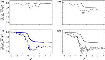
Normalized exact
 $\overline{\overline{F^{E}}}/\overline{\overline{F_{1}^{E}}}$
(——) and approximated
 $(\overline{\overline{F^{E}}}/\overline{\overline{F_{1}^{E}}})_{apx1}\approx \overline{\overline{{\it\eta}^{2}}}/\overline{\overline{{\it\eta}_{1}^{2}}}$
(– – –) averaged horizontal energy flux for intermediate-depth (a) incipient breaking, RI; (b) spilling breaker, RS1; (c) plunging breaker, RP1; and (d) plunging breaker, RP2. Circles are the measured
 $\overline{\overline{{\it\eta}^{2}}}/\overline{\overline{{\it\eta}_{1}^{2}}}$
adopted from Rapp & Melville (Reference Rapp and Melville1990) figure 11(b). Thick lines are the results for RP1(3-D).

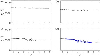
Normalized averaged energy flux due to dynamic pressure,
 $\overline{\overline{F_{p}^{E}}}/\overline{\overline{F^{E}}}$
(——), and kinetic energy
 $\overline{\overline{F_{k}^{E}}}/\overline{\overline{F^{E}}}$
(– – –) for intermediate depth (a) non-breaking packet RN; (b) incipient breaking, RI; (c) spilling breaker, RS1; and (d) plunging breaker, RP1. Thick lines are the results for RP1(3-D). Here,
 $\overline{\overline{F_{p}^{E}}}=\overline{\overline{\int _{-d}^{{\it\eta}}[p+{\it\rho}gz]u\,\text{d}z}}$
and
 $\overline{\overline{F_{k}^{E}}}=\overline{\overline{\int _{-d}^{{\it\eta}}[({\it\rho}u_{i}^{2})/2]u\,\text{d}z}}$
.

The spatial variations of
 $\overline{\overline{F^{E}}}$
are shown in figure 4 (solid lines) for different packets. Most of the energy flux loss occurs within one wavelength downstream of the break point,
 $0<x^{\ast }<1$
, while the rate of loss is larger close to the break point. The apparent loss before
 $x^{\ast }=0$
in (d) is due to a weaker preceding breaking event in the packet. For breaking packets, the contribution of the kinetic energy flux,
 $\overline{\overline{F_{k}^{E}}}=\overline{\overline{\int _{-d}^{{\it\eta}}[({\it\rho}u_{i}^{2})/2]u\,\text{d}z}}$
, to
 $\overline{\overline{F^{E}}}$
is negligibly small far from the break point, less than 3 % of the total flux, but reaches up to
 $0.15\overline{\overline{F^{E}}}$
close to the break point, as shown in figure 5. Consistent with the linear theory prediction, the contribution of
 $\overline{\overline{F_{k}^{E}}}$
to
 $\overline{\overline{F^{E}}}$
is negligibly small for the non-breaking packet RN, shown in (a).
Under the linear potential flow assumption, it is known that the averaged wave horizontal energy flux and energy density can be related using a group velocity based on the linear dispersion relation. Thus, we define an energy transport velocity for our nonlinear and breaking packets as
 $$\begin{eqnarray}C_{E}=\overline{\overline{F^{E}}}/\overline{\overline{E}},\end{eqnarray}$$
where
 $\overline{\overline{F^{E}}}$
and
 $\overline{\overline{E}}=\overline{\overline{E_{p}}}+\overline{\overline{E_{k}}}$
are the exact averaged energy flux and density calculated from the simulation results using (4.1) and (3.2), respectively. Strictly speaking, the strong nonlinearity as well as breaking-induced current and turbulent motions, which do not have a dispersion relation, make the linear potential flow assumption invalid, and thus this definition of
 $C_{E}$
is different from the theoretical definition of a linear wave group velocity, e.g.
 $C_{g}=\partial {\it\omega}/\partial k$
in the breaking region. Far from the break point, however,
 $C_{E}\simeq C_{g}$
.
The estimation of potential energy is challenging in regions where a multi-valued surface and/or large bubble void fraction exist. In other words,
 $({\it\rho}^{l}g\overline{\overline{{\it\eta}^{2}}})/2$
is only an approximate measure of the exact averaged potential energy density given by
 $\overline{\overline{E_{p}}}=\overline{\overline{\int _{-d}^{{\it\eta}}{\it\rho}gz\,\text{d}z}}+({\it\rho}^{l}gd^{2})/2$
in the regions of jet formation and subsequent splashes, which are limited in the range
 $-0.2<x^{\ast }<0.5$
in our breaking packets. Consistent with experimental studies, we use the
 $({\it\rho}^{l}g\overline{\overline{{\it\eta}^{2}}})/2$
estimation for
 $\overline{\overline{E_{p}}}$
only in our approximate formulas. Our methodology to define the free surface location in the regions with a multi-valued surface together with the comparison between
 $\overline{\overline{E_{p}}}$
and
 $({\it\rho}^{l}g\overline{\overline{{\it\eta}^{2}}})/2$
are presented in appendix A. In conclusion,
 $({\it\rho}^{l}g\overline{\overline{{\it\eta}^{2}}})/2$
is a fairly accurate estimation for
 $\overline{\overline{E_{p}}}$
except for
 $-0.2<x^{\ast }<0.5$
.
Temporal variations of surface elevation for (a) intermediate-depth plunger RP1 and (b) deep-water plunder TP2 at different spatial locations. Different lines show
 $\text{d}x^{\ast }/\text{d}t^{\ast }=C$
, where
 $C=C_{E}$
, energy transport velocity (——),
 $C=C_{gs}$
, spectrally weighted group velocity (– – –), and
 $C=C_{gc}$
, group velocity of the centre frequency of the wave packet (— ⋅ —). Circles show the crest maximum at each spatial location. For clarity, the surface elevation is exaggerated by a factor of 4.

The total loss of the averaged horizontal wave energy flux in the breaking region can be obtained as
 ${\rm\Delta}\overline{\overline{F^{E}}}=\overline{\overline{F_{1}^{E}}}-\overline{\overline{F_{2}^{E}}}$
, where the subscripts 1 and 2 refer to upstream and downstream of the break point respectively. By assuming that the averaged energy density is equal to twice the averaged potential energy density and using (4.2), we obtain
 $$\begin{eqnarray}{\rm\Delta}\overline{\overline{F^{E}}}\approx {\it\rho}^{l}gC_{E1}\left(\overline{\overline{{\it\eta}_{1}^{2}}}-\frac{C_{E2}}{C_{E1}}\,\overline{\overline{{\it\eta}_{2}^{2}}}\right),\end{eqnarray}$$
where either the linear group velocity of the centre frequency component,
 $C_{gc}$
, or a spectrally weighted group velocity of the wave packet have been previously proposed as an estimation for the characteristic group velocity. Drazen et al. (Reference Drazen, Melville and Lenain2008) defined a spectrally weighted group velocity,
 $C_{gs}$
, as
 $$\begin{eqnarray}C_{gs}=\frac{\displaystyle \sum C_{gi}|\mathscr{F}_{i}|^{2}{\rm\Delta}f_{i}}{\displaystyle \sum |\mathscr{F}_{i}|^{2}{\rm\Delta}f_{i}},\end{eqnarray}$$
where
 $C_{gi}$
is the linear group velocity of the
 $i$
th component of the wave train, and the rest of variables were defined in (2.3). They showed that their wave trains propagated at a speed close to this characteristic group velocity. Figure 6 also demonstrates that both
 $C_{E}$
and
 $C_{gs}$
are reasonable estimators of the travel speed of the wave groups, while
 $C_{gc}$
significantly underestimates wave group travel speed (see also Tian et al.
Reference Tian, Perlin and Choi2010, figure 4). In a number of previous experimental studies (Rapp & Melville Reference Rapp and Melville1990; Wu & Nepf Reference Wu and Nepf2002; Banner & Peirson Reference Banner and Peirson2007; Tian et al.
Reference Tian, Perlin and Choi2010, Reference Tian, Perlin and Choi2012), it has been assumed that
 $C_{E2}=C_{E1}$
. Thus, the total loss of the averaged horizontal wave energy flux and its associated fractional loss may be approximated as
 $$\begin{eqnarray}({\rm\Delta}\overline{\overline{F^{E}}})_{apx1}\approx {\it\rho}^{l}gC_{gs1}{\rm\Delta}\overline{\overline{{\it\eta}^{2}}},\quad ({\rm\Delta}\overline{\overline{F^{E}}}/\overline{\overline{F_{1}^{E}}})_{apx1}\approx {\rm\Delta}\overline{\overline{{\it\eta}^{2}}}/\overline{\overline{{\it\eta}_{1}^{2}}}.\end{eqnarray}$$
Figure 4 shows
 $\overline{\overline{F^{E}}}/\overline{\overline{F_{1}^{E}}}$
and
 $(\overline{\overline{F^{E}}}/\overline{\overline{F_{1}^{E}}})_{apx1}\approx \overline{\overline{{\it\eta}^{2}}}/\overline{\overline{{\it\eta}_{1}^{2}}}$
for the intermediate-depth incipient breaking RI, spilling breaker RS1 and plunging breakers, RP1 and RP2. First, 2-D simulations give fairly reasonable results in terms of the averaged horizontal energy flux and potential energy density variations compared with the corresponding 3-D simulation shown in (c) as well as the measurement shown in (d), and also provide fairly accurate results compared with the surface measurements by Tian et al. (Reference Tian, Perlin and Choi2012) for deep-water packets (not shown). The apparent undulations in
 $\overline{\overline{{\it\eta}^{2}}}$
do not exist in
 $\overline{\overline{F^{E}}}$
. Because of these undulations, a spatially averaged value of
 $\overline{\overline{{\it\eta}^{2}}}$
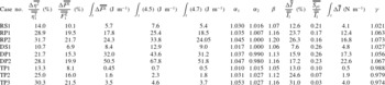
over about two meters is used upstream and downstream of the break point to apply (4.5). As summarized in table 2, using (4.5) overestimates the fractional and total loss of the horizontal energy flux by approximately 35–70 % for our breaking packets.
Three main assumptions are involved in (4.5): (i)
 $\overline{\overline{E}}\approx {\it\rho}^{l}g\overline{\overline{{\it\eta}^{2}}}$
is a valid estimation, (ii) using
 $C_{gs}$
is a sufficient estimate of
 $C_{E}$
, and (iii) the change of a selected group velocity through the breaking region may be ignored. As shown in figures 7 and 17, the first assumption is fairly accurate far from the break point (
 $x^{\ast }<-0.5$
and
 $x^{\ast }>2$
). The other two assumptions will be discussed in the following section.
Normalized averaged kinetic energy density,
 $\overline{\overline{E_{k}^{\ast }}}$
, (——); and potential energy density,
 $\overline{\overline{E_{p}^{\ast }}}$
, (– – –) for intermediate depth (a) non-breaking packet RN; (b) incipient breaking, RI; (c) spilling breaker, RS1; and (d) plunging breaker, RP1. Thick lines are the results for RP1(3-D). The results are normalized by a reference value of
 ${\it\rho}^{l}gk_{s0}^{2}S_{s0}^{-2}$
, where
 $S_{s0}$
and
 $k_{s0}$
are defined in § 4.3.

Energy transport velocity,
 $C_{E}$
, (——) and spectrally weighted group velocity,
 $C_{gs}$
(– – –) for intermediate depth (a) non-breaking packet RN; (b) incipient breaking, RI; (c) spilling breaker, RS1; and (d) plunging breaker, RP1. Thick lines are the results for RP1(3-D).

Summary of fractional and total energy and momentum flux loss for the breaking packets.
 ${\rm\Delta}\overline{\overline{{\it\eta}^{2}}}/\overline{\overline{{\it\eta}_{1}^{2}}}$
is the fractional loss of the total potential energy,
 ${\rm\Delta}\overline{\overline{F^{E}}}/\overline{\overline{F_{1}^{E}}}$
and
 $\int _{t}{\rm\Delta}\overline{\overline{F^{E}}}$
are the fractional and total loss of the total horizontal energy flux respectively,
 ${\rm\Delta}\overline{\overline{I}}/\overline{\overline{I_{1}}}$
and
 $\int _{t}{\rm\Delta}\overline{\overline{I}}$
are the fractional and total loss of the total horizontal wave momentum flux respectively.
 $\overline{\overline{S_{p1}}}$
is the horizontal momentum flux due to the mean pressure field.
 $\int _{t}$
(4.5) and
 $\int _{t}$
(4.7) are the commonly used and the proposed estimates of
 $\int _{t}{\rm\Delta}\overline{\overline{F^{E}}}$
, respectively.
 ${\it\alpha}_{1},{\it\alpha}_{2}$
and
 ${\it\beta}$
are defined below (4.6).
 ${\it\gamma}$
is defined below (5.4). Subscript
 $1$
refers to far upstream of the break point.

4.1. Characteristic wave group velocity
Figure 8 shows the spatial variation of
 $C_{E}$
(solid lines) and
 $C_{gs}$
(dashed lines), calculated using (4.2) and (4.4), for the intermediate-depth non-breaking packet RN, incipient breaking RI, as well as breaking packets RS1 and RP1.
 $C_{gs}$
is easily computed based on measured free surface time series, while estimating
 $C_{E}$
requires instantaneous velocity and pressure measurement over the entire depth. For all the breaking and non-breaking packets, there is a local increase of
 $C_{E}$
as the packets approach the focal/break point, where local peaks become relatively smaller as
 $S$
decreases. Far downstream of the focal/break point,
 $C_{E}$
is equal to its value at the upstream of the focal point for the non-breaking packet RN and the incipient breaking RI. For breaking packets, on the other hand, there is an apparent increase after the break point, due to noticeable breaking-induced dissipation of higher-frequency components of the packet. This increase of
 $C_{E}$
after the breaking region becomes relatively larger as the breaker intensity increases. Tian et al. (Reference Tian, Perlin and Choi2010) also observed a jump about a 5–10 % increase in
 $C_{gs}$
after wave breaking for their breaking packets. On the other hand, this jump is not reported by Drazen et al. (Reference Drazen, Melville and Lenain2008), who argued that their spectrally weighted group velocity remains unchanged within their experimental accuracy. Figure 8 shows that
 $C_{gs}$
is a good choice for an energy transport velocity, because it predicts fairly comparable estimates of
 $C_{E}$
before and after the breaking region.
Thus, ignoring the change of a selected wave group velocity after the breaking region leads to the overprediction of
 ${\rm\Delta}\overline{\overline{F^{E}}}$
(table 2). We can rewrite (4.3) based on
 $C_{gs}$
as
 $$\begin{eqnarray}{\rm\Delta}\overline{\overline{F^{E}}}\approx {\it\rho}^{l}gC_{gs1}({\it\alpha}_{1}\overline{\overline{{\it\eta}_{1}^{2}}}-{\it\alpha}_{2}{\it\beta}\,\overline{\overline{{\it\eta}_{2}^{2}}}),\end{eqnarray}$$
where
 ${\it\alpha}_{1,2}=(C_{E}/C_{gs})_{1,2}$
and
 ${\it\beta}=C_{gs2}/C_{gs1}$
, with
 ${\it\beta}>1.0$
can be obtained for each specific breaker using free surface measurements. Table 2 summarizes the computed values of
 ${\it\alpha}_{1},{\it\alpha}_{2}$
and
 ${\it\beta}$
for the different breaking packets. By choosing
 ${\it\alpha}_{2}=1.0$
, we get
 $$\begin{eqnarray}({\rm\Delta}\overline{\overline{F^{E}}})_{apx2}\approx {\it\rho}^{l}gC_{gs1}({\it\alpha}_{1}\overline{\overline{{\it\eta}_{1}^{2}}}-{\it\beta}\,\overline{\overline{{\it\eta}_{2}^{2}}}).\end{eqnarray}$$
where
 ${\it\alpha}_{1}=\text{Max}(1.0,0.13(S_{s0}-0.2)+1.0)$
, obtained based on linear curve fitting. Here,
 $S_{s0}$
is the spectrally weighted global steepness of the packet far upstream of breaking as defined in § 4.3. The estimated total horizontal wave energy flux losses using (4.7) are also given in table 2. In contrast to
 $({\rm\Delta}\overline{\overline{F^{E}}})_{apx1}$
, which has at least 35 % error,
 $({\rm\Delta}\overline{\overline{F^{E}}})_{apx2}$
is more accurate, with errors of less than 5 %.
Normalized energy transport velocity
 $C_{E}^{\ast }=(C_{E}-C_{gs1})/C_{gs1}$
(——), normalized wave asymmetry near the dominant component of the packet
 $As^{\ast }=0.25As/|As|_{max}$
(
 $\cdots \cdots$
), and normalized spectrally weighted frequency
 $f_{s}^{\ast }=(\,f_{s}-f_{s1})/f_{s1}$
(– – –) for intermediate depth (a) non-breaking packet RN; (b) incipient breaking, RI; (c) spilling breaker, RS1; and (d) plunging breaker, RP1.

4.2. Nonlinear wave–wave interaction before the focal/break point
Although
 $C_{gs}$
captures the main features of
 $C_{E}$
, there is a permanent lag between the local peaks of
 $C_{gs}$
and
 $C_{E}$
. In addition,
 $C_{gs}$
predicts slightly smaller values compared with
 $C_{E}$
especially before the break point, consistent with the observation of envelope propagation shown in figure 6 and by Tian et al. (Reference Tian, Perlin and Choi2010, figure 4). Tian et al. (Reference Tian, Perlin and Choi2010) found that a nonlinear correction to the linear group velocity, used to calculate
 $C_{gs}$
, had negligibly small effects and argued that this difference should be explained by nonlinear interaction between different wave components rather than the nonlinear correction to the linear group velocity of each wave component.
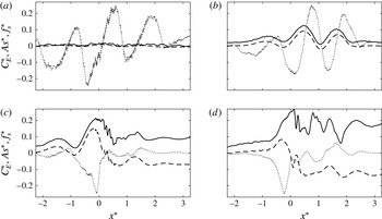
Figure 9 shows that there is an interesting correlation between these local peaks of
 $C_{E}$
before the focal/break points (solid lines) and the wave asymmetry of the dominant wave in the packet
 $A_{s}(x)=\int _{t_{zu}}^{t_{max}}{\it\eta}^{3}\,\text{d}t-\int _{t_{max}}^{t_{zd}}{\it\eta}^{3}\,\text{d}t$
(dotted lines); in which negative asymmetry, indicating waves which are pitched forward, is associated with the increase of
 $C_{E}$
and vice versa. Here,
 $t_{zu}$
and
 $t_{zd}$
are the associated time of two consecutive zero-crossing
 ${\it\eta}=0$
before and after the crest maxima at
 $t_{max}$
. The negative asymmetry can explain the observed energy transfer to the higher-frequency components, and the increase of the spectrally weighted frequency of the packet
 $f_{s}$
(dashed lines). Since the higher-frequency components have relatively smaller linear group velocities, one may expect the decrease of
 $C_{E}$
as
 $f_{s}$
increases, as predicted by
 $C_{gs}$
shown in figure 8 (dashed lines). Surprisingly,
 $C_{E}$
considerably increases as
 $f_{s}$
increases close to the focal/break points, which is completely an opposite trend compared with that predicted using the linear theory.
In the following we use the continuous wavelet transform to study the spatio-temporal structure and relative phasing of different wave components in the packet. We particularly aim to explain the considerable increase of
 $C_{E}$
before the break point
 $x^{\ast }<0$
as well as the noticeable undulation of
 $C_{E}$
in the incipient breaking case RI, as shown in figures 8 and 9 (solid lines). Because there is negligibly small breaking-induced dissipation in RI and in
 $x^{\ast }<0$
for breaking packets, this increase of
 $C_{E}$
can only be explained through the nonlinear interaction of different wave components of the packet.
The continuous wavelet transform
 $W_{\langle {\it\eta}\rangle }$
of a discrete sequence of the free surface time series at certain location,
 $\langle {\it\eta}(t)\rangle$
, is defined as the convolution of
 $\langle {\it\eta}(t)\rangle$
with a scaled and translated version of a mother wavelet
 ${\it\phi}$
,
 $$\begin{eqnarray}W_{\langle {\it\eta}\rangle }(s,t)=\frac{1}{\sqrt{s}}\int _{-\infty }^{\infty }\langle {\it\eta}({\it\tau})\rangle {\it\phi}^{\star }\left(\frac{{\it\tau}-t}{s}\right)\text{d}{\it\tau},\end{eqnarray}$$
where
 $t$
is time,
 $s=({\it\theta}f)^{-1}$
is the scale factor,
 ${\it\theta}=4{\rm\pi}/({\it\omega}_{0}+\sqrt{2+{\it\omega}_{0}^{2}})$
is a constant,
 ${\it\tau}$
is the translation factor,
 $\sqrt{s}$
is for energy normalization across different scales and
 $^{\star }$
denotes the complex conjugate. The wavelet kernel adopted here is the Morlet wavelet
 ${\it\phi}(t)=\text{e}^{\text{i}{\it\omega}_{0}t}\text{e}^{-(t^{2}/2)}$
(Farge Reference Farge1992), where
 ${\it\omega}_{0}$
is the non-dimensional central frequency of the analysing wavelet. The wavelet transform is computed in Fourier space to obtain an arbitrary number and distribution of scales.
Modulus of the wavelet transform of the non-breaking packet RN (a,c,e,g,i,k,m); and plunging breaker RP1 (b,d,f,h,j,l,n). Contours show
 $|W_{\langle {\it\eta}\rangle }|$
, in the range 0.025–0.5 with intervals of 0.025. Horizontal dotted lines show the frequency band boundaries of the input packet;


 $x^{\ast }=3.2$
(a,b); 1.6 (c,d); 0.8 (e,f); 0 (g,h);
 $-0.8$
(i,j);
 $-1.6$
(k,l); 3.2 (m,n).

Phase angle
 ${\it\Theta}_{B_{\langle {\it\eta}\rangle }}$
of the free surface bispectrum
 $B_{\langle {\it\eta}\rangle }(s_{1},s_{1},t)$
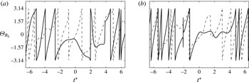
), for the non-breaking packet RN (– – –); and plunging breaker RP1 (——) at (a)
 $x^{\ast }=-0.3$
; and (b)
 $x^{\ast }=1.3$
. Here,
 $s_{1}=({\it\theta}\,f_{1})^{-1}$
,
 $f_{1}=f_{c}$
is the centre frequency, and
 ${\it\theta}=4{\rm\pi}/({\it\omega}_{0}+\sqrt{2+{\it\omega}_{0}^{2}})$
is a constant.

The modulus of the wavelet transforms of the weakly nonlinear non-breaking packet, RN, and the plunging breaker, RP1, are shown in figure 10. Except the cross-section at
 $x^{\ast }=0$
, all the
 $x$
locations shown for RP1 are outside of the region in which the surface is multi-valued. In RN, the results follow the linear theory prediction in which all the frequencies in the packet arrive at the predefined focal point,
 $x_{b}$
, at the predefined time,
 $t_{b}$
. In addition, energy at each frequency component propagates with its corresponding linear group velocity before and after the focal point, leading to symmetry of the results about
 $x^{\ast }=0$
. In RP1, however, as the packet approaches the break point, nonlinear effects lead to faster propagation of the energy, generating a permanent lead in arrival time relative to the linear prediction. In addition, a phase locking can be seen which starts from near the break point up to
 $x^{\ast }\approx 2$
, and nearly all of the frequencies propagate together with the speed close to the linear group velocity of the low-frequency components of the packet.
Strictly speaking, phase locking occurs if two frequencies, say
 $f_{1},f_{2}$
, are simultaneously present in the signal along with their sum frequency,
 $f_{3}=f_{1}+f_{2}$
, with
 ${\it\Theta}_{3}={\it\Theta}_{1}+{\it\Theta}_{2}+\text{const.}$
, where
 ${\it\Theta}_{i}$
is a corresponding phase of
 $f_{i}$
. This phase locking process in the breaking region is further demonstrated by looking at the first higher-order spectrum, or bispectrum, of the wavelet transform near the peak frequency of the wave packet. The bispectrum is defined as
 $$\begin{eqnarray}B_{\langle {\it\eta}\rangle }(s_{1},s_{2},t)=W_{\langle {\it\eta}\rangle }(s_{1},t)W_{\langle {\it\eta}\rangle }(s_{2},t)W_{\langle {\it\eta}\rangle }^{\ast }(s_{3},t),\end{eqnarray}$$
with
 $1/s_{1}+1/s_{2}=1/s_{3}$
corresponding to addition of frequencies. This analysis tool was first introduced by Van Milligen, Hidalgo & Sanchez (Reference Van Milligen, Hidalgo and Sanchez1995) in an integrated form with respect to time,
 $\int _{T}B_{\langle {\it\eta}\rangle }(s_{1},s_{2},{\it\tau})\,\text{d}{\it\tau}$
, which was shown to measure the amount of phase locking in the interval
 $T$
between wavelet components of scale lengths
 $s_{1}$
,
 $s_{2}$
and
 $s_{3}$
or equivalently of frequencies
 $f_{1},f_{2}$
and
 $f_{3}$
. We set
 $s_{1}=s_{2}$
, then
 $s_{3}=s_{1}/2$
or
 $f_{1}=f_{2}=f_{3}/2$
. Here,
 $s_{1}$
is the corresponding scale for a frequency near the peak frequency of the signal. Note that the bispectrum is a complex number, and its phase represents
 ${\it\Theta}_{B_{\langle {\it\eta}\rangle }}={\it\Theta}_{1}+{\it\Theta}_{2}-{\it\Theta}_{3}$
. In a decoupled linear system,
 ${\it\Theta}_{B_{\langle {\it\eta}\rangle }}$
changes continuously between
 $-{\rm\pi}$
to
 ${\rm\pi}$
. In the case of phase locking, however, it becomes constant or nearly so over the interval in which phase locking is occurring. Figure 11 shows
 ${\it\Theta}_{B_{\langle {\it\eta}\rangle }}$
corresponding to the centre frequency for RN and RP1 at two different
 $x$
locations. In RP1, phase locking starts upstream of the break point, and lasts for more than two wave periods in the breaking region. In RN, on the other hand, there is not such a strong phase locking and
 ${\it\Theta}_{B_{\langle {\it\eta}\rangle }}$
continuously changes between
 $-{\rm\pi}$
to
 ${\rm\pi}$
. The existence of phase locking near the centre frequency in RP1 supports the results from the wavelet analysis in a more quantitative sense.
In conclusion, the phase locking of the higher-frequency components to the lower-frequency components (e.g. as shown for RP1 figures 10 and 11), which have greater linear group velocities, leads to a considerable increase of
 $C_{E}$
before the focal/break points in the packets considered here, up to
 ${\approx}$
30 % increase compared with its values upstream of the break point.
4.3. Parameterization of the averaged breaking-induced wave energy dissipation rate
Based on scaling arguments, Duncan (Reference Duncan1983) showed that the wave energy dissipation rate per unit length of breaking crest,
 ${\it\epsilon}$
, can be written in the form
 $$\begin{eqnarray}{\it\epsilon}=b{\it\rho}^{l}g^{-1}c_{b}^{5},\end{eqnarray}$$
where
 $b$
is a breaking strength parameter, and
 $c_{b}$
is the phase speed of the breaking wave. Hereafter, the subscript
 $b$
refers to the breaking-onset instant at which a vertical tangent develops near the wave crest (
 $t_{b}^{\ast }=-0.2{-}0$
). As described by Derakhti & Kirby (Reference Derakhti and Kirby2014a
, § 4.3), the dissipation rate during active breaking has strong temporal and spatial variations, and thus using a time-invariant
 $b$
in any formulation such as (4.10) may provide an averaged estimate of the energy dissipation rate during active breaking. The averaged wave energy dissipation rate during active breaking can be approximated as
 $$\begin{eqnarray}{\it\epsilon}=\frac{\displaystyle \int _{t}{\rm\Delta}\overline{\overline{F_{br}^{E}}}}{{\it\tau}_{b}},\end{eqnarray}$$
where
 $\int _{t}{\rm\Delta}\overline{\overline{F_{br}^{E}}}$
is the total horizontal wave energy flux loss only due to breaking (see appendix B),
 ${\it\tau}_{b}={\it\alpha}_{t}T_{b}$
is a time scale related to the active breaking period and is of the order of the breaking wave period
 $T_{b}$
,
 ${\it\alpha}_{t}$
is a constant in the range
 $0.5{-}1.0$
. To estimate
 $T_{b}$
and
 $c_{b}$
, we first estimate the local wavenumber,
 $k_{b}$
, as defined in figure 1. Then, the linear dispersion relation is used to estimate the breaking wave phase speed and period as
 $c_{b}=(g/k_{b}\tanh k_{b}d)^{1/2}$
and
 $T_{b}=2{\rm\pi}/k_{b}c_{b}$
. We found
 $c_{b}/c_{s0}=0.85{-}0.90$
in our breaking packets. Because no particular choice of
 ${\it\alpha}_{t}$
gives the actual time-averaged breaking-induced dissipation rate, we set
 ${\it\alpha}_{t}=0.75$
for all cases which is consistent with Drazen et al. (Reference Drazen, Melville and Lenain2008, figure 10). Rearranging (4.10) and using (4.11), the breaking strength parameter is written as
 $$\begin{eqnarray}b=\frac{g\displaystyle \int _{t}{\rm\Delta}\overline{\overline{F_{br}^{E}}}}{{\it\rho}^{l}c_{b}^{5}{\it\tau}_{b}}.\end{eqnarray}$$
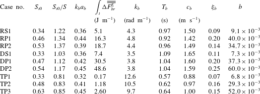
All the breaking parameters for the focused wave packets are summarized in table 3. For a packet with multiple breaking events, e.g. RP2 and TP3, the given parameters are associated with the strongest breaker of that packet. Figure 12 shows the variation of
 $b$
with respect to the local wave steepness at breaking onset
 $k_{b}a_{b}$
, and to the diagnostic parameter
 ${\it\xi}_{b}$
for different breaking packets. The solid circles are the corresponding results for the breaking waves due to modulational instability; their input parameters are given in appendix C. These local parameters can be fairly accurately estimated in phase-resolving nonlinear wave models, such as pseudo-spectral wave models (West et al.
Reference West, Brueckner, Janda, Milder and Milton1987; Goullet & Choi Reference Goullet and Choi2011; Tian et al.
Reference Tian, Perlin and Choi2012). For our focused wave packets,
 $b$
linearly decreases as
 $k_{b}a_{b}$
decreases, where
 $k_{b}a_{b}\approx 0.32$
at incipient breaking. This trend does not exist for the spilling breakers due to modulational instability, indicating
 $k_{b}a_{b}$
is not a reliable criterion neither for breaking-onset prediction or parameterization of
 $b$
. Large values of local steepness, say
 $k_{b}a_{b}>0.4$
, have been also observed by Allis (Reference Allis2013) for their very weak spillers due to modulational instability. In addition, several experimental studies (Wu & Nepf Reference Wu and Nepf2002; Allis Reference Allis2013) showed that local geometric parameters are sensitive to the degree of directionality.
Summary of the breaking parameters.
 $S_{s0}$
is the spectrally weighted global steepness of the wave packet far upstream of breaking given by (4.13),
 $S$
is the theoretical linear global steepness of a wave packet defined in § 2,
 $k$
and
 $a$
are the local wavenumber and amplitude as defined in figure 1,
 $\int _{t}{\rm\Delta}F_{br}^{E}$
is the total loss of the total horizontal energy flux due to breaking,
 $T_{b}$
and
 $c_{b}$
are the breaking wave period and phase speed respectively, and are calculated based on
 $k_{b}$
and using linear dispersion relation,
 ${\it\xi}$
is the local dynamic parameter defined in § 3 and
 $b$
is the breaking strength parameter given by (4.12). Subscript
 $b$
refers to the breaking-onset instant at which a vertical tangent develops near the wave crest, where
 $t_{b}^{\ast }=-0.2{-}0$
.

The diagnostic dynamic parameter
 ${\it\xi}_{b}$
, on the other hand, increases systematically from
 $0.048$
in the weakest spiller due to modulational instability up to
 $0.25$
in the strongest plunger due to dispersive focusing. A linear correlation between
 $b$
and
 ${\it\xi}_{b}$
exists as shown in figure 12(b), given by
 $$\begin{eqnarray}b=0.3({\it\xi}_{b}-0.05).\end{eqnarray}$$
The threshold value of 0.05 is consistent with the corresponding
 ${\it\xi}_{b}$
values for our incipient breaking packets. Banner & Peirson (Reference Banner and Peirson2007) also observed an approximately linear relationship between their diagnostic parameter just prior to wave breaking,
 ${\it\delta}_{b}$
, and
 $b$
as shown in their figure 8(b).
Variations of the breaking strength parameter
 $b$
with respect to (a) the local wave steepness at breaking onset
 $k_{b}a_{b}$
, and (b) the dynamic diagnostic parameter
 ${\it\xi}_{b}$
for (open circles) the unsteady dispersive focused breaking packets and (solid circle) the modulated unstable breaking packets; their input parameters are given in appendix C. Dashed lines are linear fits through the results of the simulated focused packets.

The parameterization of
 $b$
based on a characteristic spectrally based global steepness of a wave packet is also of an interest, especially for use in wave-averaged models where
 ${\it\xi}_{b}$
cannot be evaluated. Following Tian et al. (Reference Tian, Perlin and Choi2010), we define the spectrally weighted global steepness of a packet as
 $$\begin{eqnarray}S_{s}=k_{s}\sum a_{n},\end{eqnarray}$$
where,
 $k_{s}=2{\rm\pi}/L_{s}$
is the spectrally weighted wavenumber and
 $a_{n}$
is the Fourier amplitude of the
 $n$
th component of the wave train. Here, we only consider Fourier components in which
 $0.25f_{s0}<f_{n}<4.0f_{s0}$
. Figure 13 shows the spatial variation of
 $S_{s}$
for different non-breaking and breaking packets. Figure 13 shows that
 $S_{s}$
has a relatively constant value far upstream of the focal/break point, say
 $x^{\ast }<-3$
, hereafter referred to as
 $S_{s0}$
. We note that
 $S_{s0}$
can be easily calculated in wave-averaged models based on wave energy spectra. It is seen that
 $S_{s0}$
for all the dispersive focused breaking packets is greater than
 $S_{s0}=0.31$
for the incipient breaking packets RI and DI (not shown). In addition,
 $S_{s}$
increases as the packet approaches the break point, consistent with the observations of Tian et al. (Reference Tian, Perlin and Choi2010). Interestingly, the corresponding values of
 $S_{s}$
after the breaking region seems to reach below the threshold value of
 $(S_{s0})_{th}=0.31$
for all the dispersive focused breaking packets. This universal post-breaking value of
 $S_{s}$
could be used as a test for any selected model for the parameterization of the breaking-induced wave energy dissipation in broad-banded deep-water packets.
Spatial variations of the spectrally weighted global steepness
 $S_{s}$
for (a) intermediate-depth nonlinear packet RN (
 $\cdots \cdots$
), incipient breaking RI (– – –), spilling breaker RS1 (— ⋅ —), plunging breaker RP1 (——); and (b) deep-water nonlinear packet TN (
 $\cdots \cdots$
), weak plunging breaker TP1 (— ⋅ —), plunging breaker TP2 (– – –), plunging breaker TP3 (——).

Variations of the breaking strength parameter
 $b$
with respect to (a) the theoretical linear slope of a wave packet
 $S=\sum k_{n}a_{n}$
; and (b) the initial spectrally weighted global steepness
 $S_{s0}=k_{s0}\sum a_{n}$
for the considered focused wave packets (open circles), the simulated spillers due to modulational instability (solid circle) and the weak spilling breaking waves in a wide tank adopted from Allis (Reference Allis2013, table 8.1) (pluses). The dashed and dotted lines in (a) are given by (4.15) and
 $b=0.16\,(S_{s0}-0.28)$
. The dashed line in (b) was given by Romero, Melville & Kleiss (Reference Romero, Melville and Kleiss2012). In Allis (Reference Allis2013) the values of
 $S={\it\Sigma}a_{i}k_{i}$
have not been calculated. We assume
 $S=S_{s0}$
for their cases.

Available estimates of
 $b$
in the previous laboratory experiments range over three order of magnitude from
 $O(10^{-4})$
for gently spillers (Banner & Peirson Reference Banner and Peirson2007; Allis Reference Allis2013) up to
 $O(10^{-1})$
for strong plungers (Melville Reference Melville1994; Drazen et al.
Reference Drazen, Melville and Lenain2008; Tian et al.
Reference Tian, Perlin and Choi2010), see for example Romero et al. (Reference Romero, Melville and Kleiss2012, figure 1). Figure 14 shows the variation of
 $b$
versus the theoretical linear slope of a wave packet
 $S$
defined in § 2 as well as
 $S_{s0}$
for the considered focused wave packets (open circles), the simulated spillers due to modulational instability (solid circle) and the weak spilling breaking waves in a wide tank by Allis (Reference Allis2013) (pluses). Here, the recent laboratory results of Allis (Reference Allis2013) are used instead of those from Banner & Peirson (Reference Banner and Peirson2007), because the characteristic global steepness of the wave packets in Allis (Reference Allis2013) were calculated far upstream of the first break, consistent with our calculation of
 $S_{s0}$
. Note that Banner & Peirson (Reference Banner and Peirson2007) calculated the characteristic global steepness just before the first break in order to exclude the viscous background losses, which were
 $O(10^{1})$
higher than that in Allis (Reference Allis2013).
For our focused wave packets,
 $b>6\times 10^{-3}$
, figure 14(a) shows that
 $b\sim S_{s0}$
, consistent with the results in Tian et al. (Reference Tian, Perlin and Choi2010, figure 10(a)) and the scaling law from Derakhti & Kirby (Reference Derakhti and Kirby2014a
, equation (4.16)). However, a linear correlation does not exist for the weaker breaking packets in which
 $b<5\times 10^{-3}$
. Drazen et al. (Reference Drazen, Melville and Lenain2008) used an inertial scaling argument indicating that wave energy dissipation depends on a local wave slope to the
 $5/2$
power. Subsequently, Romero et al. (Reference Romero, Melville and Kleiss2012) showed that, within the scatter of the experimental data, a relation
 $b=0.4(S-0.08)^{5/2}$
fit the considered laboratory data in the range
 $8\times 10^{-5}<b<9\times 10^{-2}$
. Figure 14 shows that using the initial spectrally weighted global steepness
 $S_{s0}$
instead of
 $S$
results in a significant decrease of the scatter of the data. As shown in figure 14(a), the new polynomial fit based on inertial scaling is given by
 $$\begin{eqnarray}b=0.3\,(S_{s0}-0.07)^{5/2},\end{eqnarray}$$
where (4.15) gives reasonable estimates of
 $b$
over the full range of different unsteady uni-directional breaking waves. As shown in figure 13, the location at which
 $S_{s0}$
is evaluated needs to be far upstream of the break point, say
 $x^{\ast }<-3$
, to remove the spatial dependency in
 $S_{s0}$
.
Other relevant physics, such as the effects of the degree of directionality and wind forcing, need to be investigated to apply (4.15) in a real sea state.
Normalized horizontal momentum flux by waves and turbulence,
 $\overline{\overline{I^{\ast }}}$
, (——); mean pressure field,
 $\overline{\overline{S_{p}^{\ast }}}$
, (– – –);
 $\overline{\overline{I_{apx}^{\ast }}}$
(— ⋅ —); and
 $\overline{\overline{(S_{p}^{\ast })}}_{apx}$
(
 $\cdots \cdots$
) for intermediate depth (a) non-breaking packet RN; (b) incipient breaking RI; (c) spilling breaker RS1; and (d) plunging breaker RP1. Thick lines are the results for RP1(3-D). The results are normalized by a reference value of
 ${\it\rho}^{l}gk_{s0}^{2}S_{s0}^{-2}$
.

5. Fractional and total losses of momentum flux
The averaged horizontal momentum flux of a 2-D wave packet per unit crest length over the time
 $t=t_{1}\rightarrow t_{2}$
,
 $\overline{\overline{F^{M}}}$
can be written as
 $$\begin{eqnarray}\overline{\overline{F^{M}}}(x)=\frac{1}{t_{2}-t_{1}}\int _{t_{1}}^{t_{2}}\left\langle \int _{-d}^{{\it\eta}}[({\it\rho}u)u+p]\,\text{d}z\right\rangle \text{d}t.\end{eqnarray}$$
By subtracting the static pressure contribution from (5.1), the total excess horizontal momentum flux, also called the radiation stress, can be defined as
 $$\begin{eqnarray}\overline{\overline{S}}=\overline{\overline{F^{M}}}-{\textstyle \frac{1}{2}}{\it\rho}^{l}g(d+\overline{\overline{{\it\eta}}})^{2}=\overline{\overline{I}}+\overline{\overline{S_{p}}},\end{eqnarray}$$
where
 $\overline{\overline{I}}=(1/t_{2}-t_{1})\int _{t_{1}}^{t_{2}}\langle \int _{-d}^{{\it\eta}}[({\it\rho}u)u]\,\text{d}z\rangle \,\text{d}t$
represents both the averaged wave horizontal momentum flux and the turbulent Reynolds stress. For a pure wave field, however,
 $\overline{\overline{I}}\approx \overline{\overline{I}}_{apx}={\it\rho}^{l}g\overline{\overline{{\it\eta}^{2}}}n$
to the second order, where here we define
 $n$
as the ratio of the characteristic group velocity over the characteristic phase speed of the packet, given by
 $$\begin{eqnarray}n=C_{gs}/c_{s},\end{eqnarray}$$
where the
 $c_{s}$
is the spectrally weighted phase speed. Figure 15 shows that
 $\overline{\overline{I}}_{apx}$
accurately predicts
 $\overline{\overline{I}}$
before and after the breaking region. Thus, the total loss of the wave horizontal momentum flux can be written as
 $$\begin{eqnarray}{\rm\Delta}\overline{\overline{I}}\approx {\rm\Delta}\overline{\overline{I}}_{apx}={\it\rho}^{l}gn_{1}(\overline{\overline{{\it\eta}_{1}^{2}}}-{\it\gamma}\,\overline{\overline{{\it\eta}_{2}^{2}}}),\end{eqnarray}$$
where
 ${\it\gamma}=n_{2}/n_{1}$
. The corresponding
 ${\it\gamma}$
values for the different cases are summarized in table 2. In addition,
 $\overline{\overline{S_{p}}}=(1/t_{2}-t_{1})\int _{t_{1}}^{t_{2}}\langle \int _{-d}^{{\it\eta}}[p]\,\text{d}z\rangle \,\text{d}t-({\it\rho}^{l}g(d+\overline{\overline{{\it\eta}}})^{2})/2$
represents the averaged horizontal momentum flux due to the mean pressure field. For a pure wave field,
 $\overline{\overline{S_{p}}}\approx (\overline{\overline{S_{p}}})_{apx}={\it\rho}^{l}g\overline{\overline{{\it\eta}^{2}}}(n-1/2)$
to the second order. Direct estimates of
 $\overline{\overline{S_{p}}}$
(dashed lines) and its corresponding approximate measure
 $(\overline{\overline{S_{p}}})_{apx}$
(dotted lines) for non-breaking RN, incipient breaking RI, spilling RS1 and plunging RP1 packets are shown in figure 15. The results show that
 $\overline{\overline{S_{p}}}$
has relatively small change after the breaking region; thus we may assume
 ${\rm\Delta}\overline{\overline{S}}\approx {\rm\Delta}\overline{\overline{I}}$
. The loss of wave radiation stress is balanced by the increase of
 $\overline{\overline{{\it\eta}}}$
after the break point. In intermediate-depth packets the fractional loss of the time-averaged horizontal momentum flux is overpredicted by approximately 11–63 % by ignoring the change of
 $n$
after the breaking region, or choosing
 ${\it\gamma}=1$
in (5.4) (see table 2). In deep-water cases, instead, the fractional loss of the time-averaged potential energy density is close to that of the time-averaged momentum flux,
 ${\rm\Delta}\overline{\overline{I}}/\overline{\overline{I_{1}}}\approx {\rm\Delta}\overline{\overline{{\it\eta}^{2}}}/\overline{\overline{{\it\eta}_{1}^{2}}}$
.
6. Conclusions
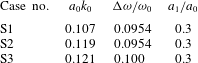
A continuum polydisperse two-fluid model described in Derakhti & Kirby (Reference Derakhti and Kirby2014a ) was used to study the breaking-onset prediction as well as the spatial variations of total energy and momentum flux in laboratory-scale intermediate- and deep-water unsteady breaking waves generated by dispersive focusing. We should remark that all the following conclusions may not be directly applicable to other types of breaking waves such as steepness-limited breaking waves due modulational instability. Also, the absolute values may need to be tested for a wider range of breaking scales. Here, we briefly establish that the present model is capable of capturing breaking waves due to modulational instability. A more detailed evaluation of this class of weak breaking events will appear in a separate paper. The main conclusions are summarized as follows.
(1) Breaking-onset prediction: Avoiding the post-processing procedure in the dimensionless parameter originally proposed by Song & Banner (Reference Song and Banner2002) given by (1.1), we defined a new diagnostic parameter,
 ${\it\xi}(t)$
, as the normalized growth rate of the time-dependent local energy density maxima along the wave packet given by
 ${\it\xi}(t)={\it\omega}_{s0}^{-1}\text{D}{\it\mu}/\text{D}t$
, where
 ${\it\mu}=E_{max}k^{2}/{\it\rho}^{l}g$
. The threshold value of
 ${\it\xi}_{th}=0.05$
was found as the maximum value of
 ${\it\xi}$
for the non-breaking and incipient breaking packets. It was shown that, the new dynamic criterion is capable of detecting a single or multiple breaking events in a packet. Noting different length scales, depth regime and packet types (see table 1) of the considered cases, the dynamic criterion with the threshold value of
 ${\it\xi}_{th}=0.05$
seems to be universal at least for steepness-limited unsteady breaking waves generated by dispersive focusing.
(2) Fractional and total losses of horizontal wave energy flux: It was shown that the widely used formulas
 ${\rm\Delta}\overline{\overline{{\it\eta}^{2}}}/\overline{\overline{{\it\eta}_{1}^{2}}}$
and
 $({\rm\Delta}\overline{\overline{F^{E}}})_{apx1}\approx {\it\rho}^{l}gC_{gs1}{\rm\Delta}\overline{\overline{{\it\eta}^{2}}}$
overpredict both fractional and total losses of horizontal wave energy flux by approximately 35–70 % for our breaking packets, due to the neglect of the increase of the characteristic group velocity after the breaking region. A new simple formulation was proposed to improve the prediction of the averaged horizontal wave energy flux as
 $({\rm\Delta}\overline{\overline{F^{E}}})_{apx2}\approx {\it\rho}^{l}gC_{gs1}({\it\alpha}_{1}\overline{\overline{{\it\eta}_{1}^{2}}}-{\it\beta}\,\overline{\overline{{\it\eta}_{2}^{2}}})$
, in which
 ${\it\alpha}_{1}=\text{Max}(1.0,0.13(S_{s0}-0.2)+1.0)$
, obtained based on linear curve fitting. Here,
 ${\it\beta}=C_{gs2}/C_{gs1}$
can be obtained based on free surface measurements upstream and downstream of the break point. The
 ${\it\beta}$
varied between 1.05 for weak spilling breakers to 1.2 for strong plunging breakers in the simulated cases.
(3) Characteristic wave group velocity: The energy transport velocity, defined as
 $C_{E}=\overline{\overline{F^{E}}}/\overline{\overline{E}}$
, was compared with the spectrally weighted linear group velocity
 $C_{gs}$
, defined by Drazen et al. (Reference Drazen, Melville and Lenain2008). In general,
 $C_{gs}$
is an appropriate choice for a characteristic group velocity, because (i) it is an easily computable quantity using only free surface time series, and (ii) it provides fairly accurate estimates of
 $C_{E}$
before and after the breaking region. However, we showed that the local peaks of
 $C_{gs}$
and
 $C_{E}$
were
 $180^{\circ }$
out of phase near the focal/break points. In addition,
 $C_{gs}$
predicts smaller values compared with
 $C_{E}$
, especially before the break point. A strong correlation between a local increase of
 $C_{E}$
and the asymmetry of the dominant wave in the packet was observed in both non-breaking and breaking packets, where negative asymmetry (wave pitched forward) led to increase of the spectrally weighted frequency,
 $f_{s}$
, of the packet, and led to a noticeable increase of
 $C_{E}$
. This increase of
 $C_{E}$
cannot be captured using linear wave theory. For example, as
 $f_{s}$
increases,
 $C_{gs}$
decreases which is completely an opposite trend compared with that observed in the results for
 $C_{E}$
. It was shown that the phase locking of the higher-frequency components to the lower-frequency components which have greater linear group velocities led to the considerable increase of
 $C_{E}$
before the focal/break points, up to
 ${\approx}$
30 % increase of
 $C_{E}$
compared with its values upstream of the break point. Far downstream of the focal point,
 $C_{E}$
returned to its value upstream of the focal point for non-breaking packets. For breaking packets, however, there is a significant increase of
 $C_{E}$
after the break point, due to noticeable breaking-induced dissipation of higher-frequency components within the wave packet. This increase became relatively larger as the breaker intensity increased.
(4) Parametrization of the breaking strength parameter
 $b$
: As summarized by Romero et al. (Reference Romero, Melville and Kleiss2012), the available estimates of
 $b$
ranges from
 $O(10^{-4})$
for gently spillers up to
 $O(10^{-1})$
for strong plungers. In most of the previous experiments,
 ${\rm\Delta}\overline{\overline{F^{E}}}$
was approximated using
 $({\rm\Delta}\overline{\overline{F^{E}}})_{apx1}\approx {\it\rho}^{l}gC_{gs1}{\rm\Delta}\overline{\overline{{\it\eta}^{2}}}$
. As we explained, using
 $({\rm\Delta}\overline{\overline{F^{E}}})_{apx2}\approx {\it\rho}^{l}gC_{gs1}({\it\alpha}_{1}\overline{\overline{{\it\eta}_{1}^{2}}}-{\it\beta}\,\overline{\overline{{\it\eta}_{2}^{2}}})$
the estimation of
 ${\rm\Delta}\overline{\overline{F^{E}}}$
and the associated
 $b$
is improved compared with that predicted using
 $({\rm\Delta}\overline{\overline{F^{E}}})_{apx1}\approx {\it\rho}^{l}gC_{gs1}{\rm\Delta}\overline{\overline{{\it\eta}^{2}}}$
. In addition, we found that the initial spectrally weighted global steepness,
 $S_{s0}$
, is a preferable parameter compared with the theoretical linear global steepness
 $S=\sum _{i=1}^{N}a_{i}k_{i}$
for our dispersive focused packets. The new diagnostic parameter at the breaking-onset,
 ${\it\xi}_{b}$
, was shown to have a strong linear dependence with respect to
 $b$
given by
 $b=0.3({\it\xi}_{b}-0.05)$
. Note that in the present work, the estimated
 $b$
ranges from
 $3\times 10^{-4}$
up to
 $0.06$
. Although
 ${\it\xi}_{b}$
cannot be evaluated in wave-averaged wave models, it can be easily used in wave-resolving nonlinear wave models. A strong linear dependence was also found between
 $b$
and
 $S_{s0}$
for the considered focused wave packets, while a large scatter was found between
 $b$
and
 $S$
. The linear relation, however, cannot provide accurate estimations of
 $b$
in the range
 $b<5\times 10^{-3}$
. A new scaling law given by
 $b=0.3(S_{s0}-0.07)^{5/2}$
, which is consistent with inertial wave dissipation scaling of Drazen et al. (Reference Drazen, Melville and Lenain2008), is shown to be capable of providing accurate estimates of
 $b$
in the full range of breaking intensities,
 $10^{-5}<b<10^{-1}$
, where the scatter of data in the new formulation significantly decreases compared with that proposed by Romero et al. (Reference Romero, Melville and Kleiss2012).
(5) Fractional and total losses of total momentum flux: Momentum flux due to the mean pressure
 $\overline{\overline{S_{p}}}$
was shown to have relatively small change after the breaking region, and, thus,
 ${\rm\Delta}\overline{\overline{S}}\approx {\rm\Delta}\overline{\overline{I}}$
. We showed that total wave momentum flux,
 $\overline{\overline{I}}$
, could be accurately estimated as
 $\overline{\overline{I}}_{apx}={\it\rho}g\overline{\overline{{\it\eta}^{2}}}n$
upstream and far downstream of the break point, where we defined
 $n=C_{gs}/c_{s}$
. In intermediate-depth breaking packets, total fractional loss of horizontal momentum flux was approximately 11–63 % overpredicted by ignoring the change of
 $n$
after the breaking region, or choosing
 ${\it\gamma}=n_{2}/n_{1}=1$
in (5.4). In deep-water cases, on the other hand, the fractional loss of the averaged potential energy density was close to that of the averaged horizontal wave momentum flux.
Snapshots of the spatial variations of the air–water interface (——) and the calculated
 ${\it\eta}(t,x)$
(

 $\text{G3}=({\rm\Delta}x=10.0,{\rm\Delta}z=5.0)$
mm. (a)
 $t^{\ast }=-0.06$
, (b) 0.06, (c) 0.17, (d) 0.28, (e) 0.39, (f) 0.50, (g) 0.61.

Spatial variations of the normalized exact,
 $2\overline{\overline{E_{p}}}/{\it\rho}^{l}g$
, (——) and approximated,
 $\overline{\overline{{\it\eta}^{2}}}$
, (

 $\text{G3}=({\rm\Delta}x=10.0,{\rm\Delta}z=5.0)$
mm. Vertical dashed lines show
 $x^{\ast }=-0.2$
and
 $x^{\ast }=0.5$
.

Acknowledgements
This work was supported by ONR, Littoral Geosciences and Optics Program (grant N00014-13-1-0124), NSF, Physical Oceanography Program (grant OCE-1435147), and through the use of computational resources provided by Information Technologies at the University of Delaware.
Appendix A. Free surface definition close to the break point
The free surface location
 ${\it\eta}(x,t)$
defined as the top air–water interface location if
 ${\it\alpha}^{l}>0.5$
is satisfied in the three adjacent computational cells below that interfacial cell. By doing this we avoid the small splashes and low void fraction regions to be considered as a free surface. Figure 16 shows snapshots of the spatial variations of the air–water interface and its associated calculated
 ${\it\eta}(x,t)$
(black lines) for the intermediate-depth plunging breaking case DP1. Figure 17 shows that the approximated time-averaged potential energy density,
 $({\it\rho}^{l}g\overline{\overline{{\it\eta}^{2}}})/2$
, based on our choice of the free surface location, has more pronounce oscillations during the jet formation between
 $-0.2<x^{\ast }<0$
compared with the exact values
 $\overline{\overline{E_{p}}}$
. For
 $x^{\ast }<-0.2$
and
 $0.5<x^{\ast }$
, the difference between
 $\overline{\overline{E_{p}}}$
and
 $({\it\rho}^{l}g\overline{\overline{{\it\eta}^{2}}})/2$
are negligibly small.
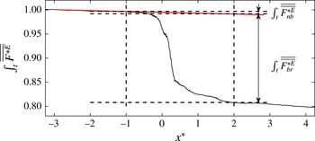
Appendix B. Estimation of wave energy dissipation due to breaking and non-breaking processes
The total loss of the horizontal wave energy flux
 $\int _{t}{\rm\Delta}\overline{\overline{F^{E}}}$
given by (4.3) includes both non-breaking, e.g. viscous dissipation due to boundaries and inside the water body, and breaking processes. In any model simulation, numerical dissipation always contributes to some of the energy loss in the system. Here, we consider the numerical dissipation as a non-breaking dissipation. To estimate the total non-breaking wave energy dissipation, we fit a line to
 $\int _{t}\overline{\overline{F^{E}}}$
upstream of the break point, we observed that this line also represents a linear fit to
 $\int _{t}\overline{\overline{F^{E}}}$
downstream of the break point. Then, we assume that
 $\int _{t}{\rm\Delta}\overline{\overline{F_{nb}^{E}}}(x^{\ast }\rightarrow x^{\ast }+1)$
which is the slope of the fitted line is constant over the whole numerical domain, including the breaking region. Thus the total non-breaking loss of the horizontal wave energy flux between
 $x_{1}$
and
 $x_{2}$
can be estimated as
 $$\begin{eqnarray}\int _{t}{\rm\Delta}\overline{\overline{F_{nb}^{E}}}(x_{1}^{\ast }\rightarrow x_{2}^{\ast })=(x_{2}^{\ast }-x_{1}^{\ast })\int _{t}{\rm\Delta}\overline{\overline{F_{nb}^{E}}}(x^{\ast }\rightarrow x^{\ast }+1),\end{eqnarray}$$
and thus
 $\int _{t}{\rm\Delta}\overline{\overline{F_{br}^{E}}}=\int _{t}{\rm\Delta}\overline{\overline{F^{E}}}-\int _{t}{\rm\Delta}\overline{\overline{F_{nb}^{E}}}$
. The values of
 $\int _{t}{\rm\Delta}\overline{\overline{F_{br}^{E}}}$
for the considered focused wave packets are given in table 3. The ratio of
 $\int _{t}{\rm\Delta}\overline{\overline{F_{nb}^{E}}}(x^{\ast }\rightarrow x^{\ast }+1)/\int _{t}{\rm\Delta}\overline{\overline{F_{br}^{E}}}$
ranges from
 ${\approx}$
0.01 up to 0.04 in our focused plunging and spilling breaking wave packets. In most of the considered cases, the decrease of the mesh resolution results in the increase of
 $\int _{t}{\rm\Delta}\overline{\overline{F_{br}^{E}}}$
and thus the increase of the breaking strength parameter
 $b$
. Table 4 summarizes the estimated
 $b$
using different mesh resolution for our focused breaking wave packets.
Calculation of the total loss of the horizontal wave energy flux due to breaking and non-breaking processes. The reference value is the total horizontal wave energy flux far upstream of the break point,
 $\int _{t}\overline{\overline{F_{1}^{E}}}$
.

Variation of the breaking strength parameter
 $b$
given by (4.12) with respect to different grid densities for simulated focused packets. Different meth grid densities are:
 $\text{G2}=({\rm\Delta}x=18.3,{\rm\Delta}z=5.0)$
mm,
 $\text{G3}=({\rm\Delta}x=10.0,{\rm\Delta}z=5.0)$
mm, and
 $\text{G4}=({\rm\Delta}x=5.0,{\rm\Delta}z=5.0)$
mm.

Appendix C. Input parameters for the breaking wave due to modulational instability
For the generation of wave packets due to modulational instability, wave packets composed of a carrier wave and one- or two side-band perturbation components are produced. Here, we follow the set-up of the bimodal initial spectrum, case II, wave packets in Allis (Reference Allis2013), which is similar to case II in Banner & Peirson (Reference Banner and Peirson2007). The surface displacement at the incident boundary
 $x=0$
is given by
 $$\begin{eqnarray}{\it\eta}(0,t)=a_{0}\cos ({\it\omega}_{0}t)+a_{1}\cos \left({\it\omega}_{1}t-\frac{{\rm\pi}}{18}\right),\end{eqnarray}$$
where
 ${\it\omega}_{0}=8.985~\text{s}^{-1}$
,
 ${\it\omega}_{1}={\it\omega}_{0}+{\rm\Delta}{\it\omega}$
. Table 5 gives the rest of input parameters for the three simulated cases. The 2-D numerical domain of (50.0, 0.64) m is discretized by a uniform grid of
 ${\rm\Delta}x=7.8$
mm and
 ${\rm\Delta}z=4$
mm.
Input parameters for the simulated breaking packets due to modulational instability. Here,
 $k_{0}=8.23~\text{m}^{-1}$
and
 $d=0.55$
m is the still water depth.