2. SPURIOUS REGRESSIONS WITH NONSTATIONARY PROCESSES

Consider the following data generating process:

where x_t and u_t are nonstationary I(d) processes such that

where d_x, d_u > ½ and ε_xt and ε_ut are two weakly dependent processes. For simplicity, we assume that x_t is a scalar process. The results of this paper easily can be extended to multivariate cases.

We further assume that x_t and u_t satisfy the following functional central limit theorem (FCLT):

where

W(s) = (W_x(s),W_u(s))′ is a bivariate Brownian motion with positive definite long-run variance

The FCLT holds under a wide range of primitive conditions (e.g., Marinucci and Robinson, 2000). When x_t and u_t are unit root processes, the limiting process V(r) = (V_x(r),V_u(r))′ reduces to a scaled Brownian motion. For a general nonstationary fractional process, the limiting process is a type II fractional Brownian motion (Marinucci and Robinson, 1999).

When d_u ≥ d_x, there is no cointegrating relationship between y_t and x_t, and we have a spurious linear model. When d_u < d_x, y_t and x_t are fractionally cointegrated with cointegrating vector (1,−β). However, because the long-run equilibrium error u_t is nonstationary, Marmol (1998) refers to the second situation as a partially spurious case. For convenience, we will refer to both cases as spurious cases.

Consider regressing y_t on a constant and x_t,

The OLS estimate of β is given by

where

. The heteroskedasiticity and autocorrelation consistent t-statistic is

, where

is the HAC estimator defined as

where

k(·) is a kernel function, and M is the bandwidth parameter.

To get a consistent estimate of the long-run variance of

, conventional asymptotic theory assumes that M → ∞ such that M = o(T). However,

is nonstationary, and the variance of

does not converge. In other words, the sum

is infinite with the probability approaching one as T → ∞. The infiniteness of this sum invalidates the usual truncation argument. As becomes clear later on, when M is taken to grow at a slower rate than T, the estimate

underestimates the variability of

by an order of magnitude. The resulting t-statistic will diverge, leading to the spurious rejection. A natural question is: what if M grows at the same rate as T? In the rest of the paper, we set M = bT for some b ∈ (0,1] and provide an answer to this question. For convenience, we call the asymptotics under the assumption of M = bT the large M asymptotics.

To ensure the positive definiteness of

, we assume that the kernel function belongs to the following class:

where

The class

is similar to class

in Andrews (1991).

The following theorem establishes the asymptotic distributions of

, and the resulting t-statistic

. The theorem uses the following notation:

and

THEOREM 1. Assume that x_t and u_t satisfy the FCLT in (3) and y_t is generated by (1). Let k(x) be a continuous function in

and M = bT for b ∈ (0,1]. Then, as T → ∞,

Theorem 1 shows that when M = bT, the HAC estimator delivers a standard error estimate that is of the same stochastic order as

. Based on such a HAC estimate, the t-statistic is stochastically bounded and converges to a well-defined distribution. In contrast, the conventional variance estimator (also called the OLS variance estimator), which is

, ignores the autocorrelation in the underlying processes and underestimates var(

) by an order of magnitude. When the OLS estimator is normalized by the conventional standard error estimate, the resulting t-statistic is bound to diverge. The rate of divergence is

, as shown by Phillips (1986) and Marmol (1998).

Our finding is consistent with a result by Phillips (1998), who considers regressing a unit root process on a complete orthonormal system in L₂ [0,1]. He shows that the t-statistic based on the usual HAC standard error with bandwidth M is of order O_p((T/M)^1/2). From this, one may deduce heuristically that when M = bT, the t-statistic is stochastically bounded, whereas when M = o(T), the t-statistic diverges at the rate of

.

Now we consider the spurious regression between a nonstationary I(d) process and a linear trend. The data generating process for u_t is the same as before so that the invariance principle in (3) holds for T^{−(2d_u−1)/2}u_[Tr]. The data generating process for x_t is replaced by x_t = t so that T^{−(2d_x−1)/2}x_[Tr] → r for

. Using arguments similar to the proof of Theorem 1, we can prove the following theorem immediately. The details are omitted.

THEOREM 2. Assume that x_t = t, u_t satisfies the FCLT in (3), and y_t = α + βt + u_t. Let k(x) be a continuous function in

and M = bT for b ∈ (0,1]. Then

where

Theorem 2 shows that when M = bT, the t-statistic is convergent, as in the case of a regression between two nonstationary fractional processes. In contrast, the usual t-statistic diverges at the rate of

(see Durlauf and Phillips, 1988; Marmol and Velasco, 2002).

Results similar to Theorem 2 have also been obtained by Marmol and Velasco (2002), who analyze the effects of spuriously detrending a nonstationary fractional process. Put in our context, they used the long-run variance estimate of the form:

where

. As a result of the difference in the construction of the variance estimate, their limiting distributions are different from ours. Nevertheless, the basic message is the same: it is necessary to let M = bT to deliver a convergent t-statistic.

Together with Theorem 1, Theorem 2 shows that when M = bT, the t-statistic converges in distribution in the spurious regression with nonstationary fractional processes. This finding implies that the t-test based on the large M asymptotics will not point to a significant relationship between two independent processes.

3. SPURIOUS REGRESSIONS WITH STATIONARY PROCESSES

In this section, we consider the regression between two stationary I(d) processes and that between a stationary I(d) process and a linear trend.

The first data generating process we consider is the same as that in Chung (2002). For completeness, we briefly describe the data generating process. We assume that y_t is generated according to

where (x_t,u_t)′ is a vector linear process defined by

ε_t = (ε_1t,ε_2t)′ is a martingale difference sequence with respect to the natural filtration

for some matrix Σ, and {Ψ_j} is a sequence of 2 × 2 matrices. As in Chung (2002), we maintain the following assumptions.

A1. For some δ > 0,

, a.s. for i = 1 and 2.

A2. For some nonsingular constant matrix Π,

where ∼ means the ratio of the left- and right-hand-side elements tends to one and Γ(·) is the gamma function.

A3. 0 < d_x,d_u < 0.5.

Define the random vector element

Under Assumptions A1–A3, the following lemma holds.

LEMMA 3. Let Assumptions A1–A3 hold. If d_x + d_u > ½, then

where

Here ξ₊^d = [max(0,ξ)]^d and (W_x(t),W_u(t))′ is a vector Brownian motion with variance matrix ΠΣΠ′.

Note that B_dx(r) and B_du(r) are type I fractional Brownian motions (Marinucci and Robinson, 1999). Lemma 3 shows that the partial sum of a fractional process converges to fractional Brownian motion. This result is not new and has been proved by numerous authors, including Davidson and de Jong (2000) and Chung (2002). Lemma 3 also shows that the partial sum of the product process x_tu_t converges to the non-Gaussian process Z(r). This result is obtained by Chung (2002, Theorem 2) but under the stronger assumption that d_x,d_u ∈ (0.25, 0.5). A careful inspection of Chung's proof reveals that his Theorem 2 holds as long as d_x + d_u > ½.

Using Lemma 3 and following the same steps as the proof of Theorem 1, we can establish the asymptotic distributions of

, and the t-statistic in the following theorem.

THEOREM 4. Let Assumptions A1–A3 hold. Assume that k(x) is a twice continuously differentiable function in

and M = bT for b ∈ (0,1]. If d_x + d_u > ½, then

where

The theorem shows when x_t and u_t are correlated, the OLS estimate of β will be inconsistent. To facilitate the comparison with the existing literature on spurious regression between stationary long memory processes, we assume σ_ux = 0 in the discussion that follows. It should be noted that when d_x > d_u, β can be consistently estimated using a frequency domain approach even if σ_ux ≠ 0 (cf. Robinson, 1994).

When σ_ux = 0, Theorem 4 reveals the convergence of the t-statistic when M = bT. In contrast, Tsay and Chung (2000) show that the t-statistic based on the OLS standard error diverges at the rate of T^{d_x+d_u−0.5}. As a consequence, the slope coefficient in the regression between two independent stationary long memory processes can be spuriously significant. The convergence of the t-statistic under the new asymptotics has profound implications. Note that the OLS estimator

is consistent, the R² converges to zero, and the Durbin–Watson (DW)-statistic does not approach zero (Tsay and Chung, 2000). The behaviors of

, R², and DW are thus the same as in the case of no spurious effect. The only qualitative difference is the divergence of the usual t-statistic. Therefore, under the large M asymptotics, all of the statistics behave as in the case of usual regression. Hence, inferences based on the large M asymptotics will not result in finding a significant relationship that does not actually exist. We may conclude that there is no spurious effect between two independent stationary long memory processes, as long as M is allowed to grow at the same rate as T and correct critical values are employed.

The preceding theorem assumes that the kernel function is twice continuously differentiable. This excludes the widely used Bartlett kernel. The following theorem establishes the asymptotic distributions of

, and the t-statistic when the Bartlett kernel is employed.

THEOREM 5. Let Assumptions A1–A3 hold. If k(x) = (1 − |x|)1{|x| ≤ 1}, M = bT for b ∈ (0,1], and d_x + d_u > ½, then Theorem 4 holds with

replaced by

Tsay and Chung (2000) show that when a stationary I(d) process is regressed on a linear trend, the usual t-statistic diverges at the rate of T^d. We proceed to investigate whether this is the case when M = bT. To this end, we assume that u_t satisfies the FCLT as before:

Using summing by parts and the continuous mapping theorem, we have

Let

Then we can prove the following theorem using (26) and (27) and arguments similar to the proof of Theorem 4. Details are omitted.

THEOREM 6. Let x_t = t and u_t satisfy (26) with d_u ∈ (0,½). If k(x) is a twice continuously differentiable function in

and M = bT for b ∈ (0,1], then

If k(x) = (1 − |x|)1{|x| ≤ 1}, then (29), (30), and (31) hold with

replaced by

Theorem 6 shows that the OLS estimator is consistent and the t-statistic converges as in other cases. Therefore, detrending a stationary fractionally integrated process will not lead to the spurious effect of finding a significant trend, as long as critical values from the large M asymptotics are used.

4. KERNEL ESTIMATES OF ASYMPTOTIC DISTRIBUTIONS

The limiting distributions of

are nonstandard. In this section, we use Monte Carlo simulations to approximate their probability densities. Our goal is to see how the new limiting distribution differs from the standard normal distribution and to what extent the use of M = bT helps reduce the spurious effects.

For simplicity, we assume that there is no correlation between {x_t} and {u_t}. In this case, it suffices to simulate simple fractionally integrated processes. Specifically, we generate the fractional processes x_t and u_t according to (1 − L)^d_xx_t = ε_xt and (1 − L)^d_uu_t = ε_ut, where ε_xt ∼ iidN(0,1), ε_ut ∼ iidN(0,1) for t > 0, ε_xt = ε_ut = 0 for t ≤ 0, and {ε_xt} is independent of {ε_ut}. Without loss of generality, we let β = 0. For spurious regressions between nonstationary I(d) processes, we consider (d_x,d_u) = (0.6, 0.6), (0.6, 1), (1, 0.6), or (1, 1), and for those between stationary ones, we let (d_x,d_u) = (0.3, 0.3), (0.4, 0.2), or (0.2, 0.4). We let k(·) be the Bartlett kernel and consider the following values of b = 0, 0.025, 0.05,…,1. When b = 0,

becomes

. We use 5,000 replications and a sample size of 1,000. For the results reported here, 10,000 replications are employed.

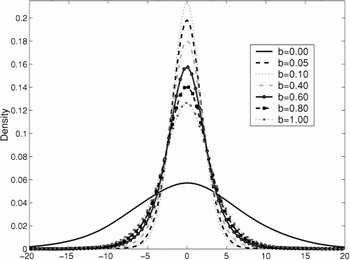
We first examine spurious regressions with nonstationary fractional processes. Figure 1 reports the kernel estimates of the probability densities for the case x_t ∼ I(d_x), u_t ∼ I(d_u) with d_x = d_u = 0.6. The qualitative results for other (d_x,d_u) combinations are similar. The probability densities appear to be symmetric and are apparently more dispersed than the standard normal density. For example, when b = 0.1, the 95% quantile of the limiting distribution is 3.1012, which is larger than 1.645, the 95% quantile of the standard normal distribution. The quantile is not a monotonic function of b. When b is small, the quantile is decreasing in b, whereas when b is large, the quantile is increasing in b. In other words, when b moves closer to zero or one, the limiting distribution becomes more dispersed. This result is well expected when b is very close to zero. In this case, the behavior of the t-statistic may be better described by the conventional limit theory. However, when b is very close to one, one may think that the limiting distribution should become less dispersed as the variance estimate with a large bandwidth captures the strong autocorrelation in x_tu_t. This is not what is happening. In fact, as b becomes close to one, the variance estimate

does not capture the strong autocorrelation very well. This is because u_t is not observed and has to be replaced by the estimated residual

. As a consequence, when k(x) = 1 and b = 1,

is zero by construction. Of course, this is an extreme case. But for other kernels, when b is close to one, the effect of increasing b is similar. The estimate

tends to bias toward zero when

incorporates autocovariances of almost all lags.

Kernel estimates of densities of when xt ∼ I(0.6) and yt ∼ I(0.6).

For all the cases considered, the simulation results indicate that the limiting distribution is least dispersed or close to being least dispersed when b = 0.1. When d_x = d_u = 0.6 and b = 0.1, the probability of

is 28.39%. Therefore, when M = 0.1T, we will erroneously reject the null 28.39% of the times when the wrong critical value is used. In contrast, when M = o(T), the rejection probability goes to one as the sample size increases. When T = 1,000 and the OLS standard error is used, the rejection probability is 75.9%, as shown by simulations. Hence, the use of M = 0.1T reduces the spurious effect substantially.

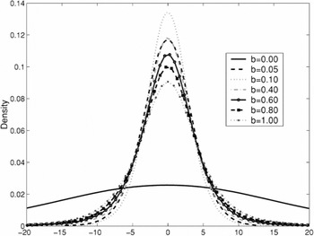
Figure 2 presents the same graph when y_t is an I(0.6) process and x_t is a linear deterministic trend. The graph is representative of other cases. The qualitative observations made for Figure 1 apply. However, the limiting distributions become more dispersed than those in Figure 1.

Kernel estimates of densities of when xt = t and yt ∼ I(0.6).

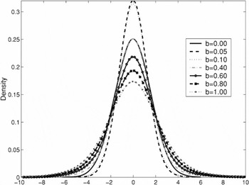
We next consider spurious regressions with stationary fractional processes. Figure 3 graphs the density estimates when (d_x,d_u) = (0.4, 0.2). The density estimates for the other two cases turn out to be close to the case (d_x,d_u) = (0.4, 0.2). The figure shows that the limiting distributions are more concentrated around the origin than in the nonstationary cases. For example, the 90% quantiles when b = 0, 0.1, 0.2, 0.3, 0.4, 0.5 are 1.9265, 1.5602, 1.6963, 1.8440, 2.0120, and 2.1654, respectively. The corresponding 95% quantiles are 2.4695, 2.0525, 2.2118, 2.4741, 2.6988, and 2.9385, respectively. Simulation results show that the limiting distribution becomes close to the standard normal when b is close to 0.1. For example, when b = 0.1, the probability of

is 11.70%, which is very close to 10%, the size of the test when

is standard normal. In other words, when M = 0.1T is used to test the null of β = 0, the probability of wrong rejection is only 11.70% even if the critical value does not come from the true limiting distribution. To a great extent, the new t-test eliminates the spurious effect.

Kernel estimates of densities of when xt ∼ I(0.4) and yt ∼ I(0.2).

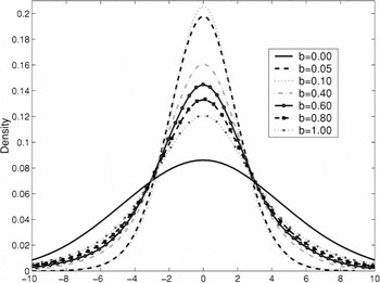
Figure 4 graphs the density estimates when y_t ∼ I(0.3) and x_t = t. Again, we find that the densities are more concentrated than in the nonstationary cases and become most concentrated when b is close to 0.1. Another feature of Figures 3 and 4 is that the densities appear to be slightly negatively skewed (skewed to the left).

Kernel estimates of densities of when xt = t and yt ∼ I(0.3).