INTRODUCTION
Over the last few decades, agricultural land use, especially intensive use of croplands, has led to significant changes in rural areas. Anthropogenic influences such as changes in land use and crop patterns, the use of heavy agricultural machinery and land consolidation have greatly increased the wind and water erosion potential of soils. In Austria, c. 0·12 of the area used for agriculture can be classified as ‘erodible land’ (Strauss & Klaghofer Reference Strauss, Klaghofer, Boardman and Poesen2006).
In eastern Austria, climate change will lead to an increase in air temperature (Formayer et al. Reference Formayer, Eitzinger, Nefzger, Simic and Kromp-Kolb2001). Simulations of future rainfall patterns show no clear trend of increase or decrease but they indicate shifts from summer to winter and spring rainfall. Semenov & Bengtsson (Reference Semenov and Bengtsson2002) concluded that, in Central Europe, the amount of precipitation will not change significantly until 2100, but the frequency of rainstorms will increase by 15%. This will also result in higher rainfall intensities and, therefore, also in increased rainfall erosivity. Nearing (Reference Nearing2001) investigated the impact of climate change on rainfall characteristics and used the output of global circulation models (GCMs) and statistical relationships on erosivity from the Revised Universal Soil Loss Equation (RUSLE model; Renard et al. Reference Renard, Foster, Weesies, McCool and Yoder1995) to compute climate-change-induced alterations on the erosive force of precipitation in the USA. Despite certain inconsistencies, the results showed critical increases in rainfall erosivity of up to 58% at some locations, which may considerably affect future soil erosion rates.
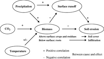
Rising air temperatures affect soil evaporation and transpiration and therefore alter the soil water balance. In addition, climate change varies growth conditions with partly positive but mainly negative effects on soil erosion. Relevant criteria include soil cover by plant canopies and plant residues as well as root growth and the content of organic carbon in the soil (Fig. 1). Higher rainfall erosivity modifies hydrological conditions and will cause an increase in surface runoff and soil erosion although land use may not be changed. Estimates by the EU indicate that as an effect of climate change, the water erosion risk is expected to increase by the year 2050 in about 0·80 of EU agricultural areas (EEA 2000). This increase will take place mainly in the areas where soil erosion is currently severe (EEA 1999).
Main pathways of selected climatic factors on surface runoff and soil erosion (modified after Pruski & Nearing Reference Pruski and Nearing2002b).

In Central Europe, soil erosion is mainly associated with the cultivation of root and/or row crops such as potatoes, sugar beets, carrots and, especially, maize (Jones et al. Reference Jones, Le Bissonnais, Diaz, Düwel, Øygarden, Bazzoffi, Prasuhn, Yordanov, Strauss, Rydell, Uveges, Loj, Lane and Vandekerckhove2003). Two main factors are responsible for this high risk: low soil and canopy cover during the time of seedbed preparation and early stages of vegetative development, and the occurrence of the most erosive storms during this time period (Strauss et al. Reference Strauss, Auerswald, Blum and Klaghofer1995).
In recent years, the Austrian Agri-Environmental Programme was established (BMLFUW 2007) to promote sustainable land management in Austria. Practices such as mulch and direct seeding are included and farmers are encouraged to adopt these measures by providing incentives. The aim of these measures is to maintain a complete soil cover throughout the whole year. Soil management systems with reduced tillage intensity in combination with cover crops during the winter are effective systems for reducing soil erosion by water (Klik Reference Klik2003) and enhancing soil quality by improving soil physical, chemical and biological properties (Hofmann Reference Hofmann2005).
The goal of the present study was to assess the effectiveness of these soil conservation measures under expected future climate scenarios, with respect to sediment yield leaving a watershed and to the availability of soil water for plant production. Specific objectives were (1) to evaluate the impacts of climate change on soil erosion and surface runoff for an area used for agriculture in the northeast of Austria, (2) to assess different land use systems with respect to soil erosion and water retention and (3) to provide regional policy makers with additional information for policy development in the agricultural and environmental sector.
MATERIALS AND METHODS
Description of the project area
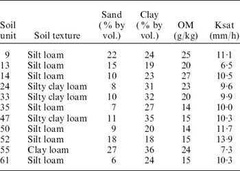
The study was carried out in a 1·14 km2 agricultural watershed in the north-east of Austria (48°34′N, 16°35′E). It is located in the so-called ‘Wine Quarter’, which is influenced by a Pannonian-Middle European transition climate. The region is one of the warmest and driest areas in Austria. Average long-term annual precipitation is 534 mm with an average annual temperature of 9·5°C. In the watershed, three soil textures can be classified which can be differentiated into 11 soil units. Sand contents range from 60 to 220 g/kg, clay contents from 180 to 320 g/kg and organic matter (OM) contents from 14 to 25 g/kg. Main soil parameters are given in Table 1.
Main physical and chemical soil parameters

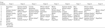
The 66 field parcels in the watershed are used as cropland, vineyard and forest. Four crop rotations typical for the region were selected and divided into 11 rotations with different starting crops (Table 2).
Main crop rotations in the watershed

* Cover crop.
Three soil management systems were selected for evaluation: (1) conventional soil tillage using a plough in the autumn and preparing a conventional seedbed (conventional tillage, CT), (2) no-till (NT) with a cover crop during winter and (3) grassland, which represents the optimum agronomic soil protection measure (Grass).
Selected climate scenarios
The climate in 1961–90 was used as the baseline period. For this, data from Gross-Enzersdorf (48°12′N, 16°33′E), located 10 km east of Vienna, Austria, were used because detailed information about current status and future scenarios are available for this station. Two climate scenarios for 2050 were used to evaluate the effectiveness of the investigated soil protection systems, viz. Intergovernmental Panel on Climate Change (IPCC) scenario A1B (ECHAM5 low and high) and IPCC scenario A2 (ECHAM4 low and high). These climate scenarios are based on two IPCC scenarios (SRES A1B and SRES A2). The A1B emission scenario assumes an integrated world where income and way of life converge between regions, with rapid economic growth, a quick spread of new and efficient technologies and a balanced emphasis on all available resources. Scenario A2 supposes a heterogeneous world where the preservation of local identities is emphasized. The global population increases steadily, economic growth and technological change are fragmented and comparatively slow, whilst greenhouse gases continue to be emitted at high rates (IPCC 2000).
The climate change scenarios are based on the transient simulations made by the GCMs ECHAM4 (Röckner et al. Reference Röckner, Arpe, Bengtsson, Christoph, Claussen, Dümenil, Esch, Giorgetta, Schlese and Schulzweida1996) and ECHAM5 (Röckner et al. Reference Röckner, Bäuml, Bonaventura, Brokopf, Esch, Giorgetta, Hagemann, Kirchner, Kornblüh, Manzini, Rhodin, Schlese, Schulzweida and Tompkins2003). The climate change scenarios were constructed by Dubrovsky et al. (Reference Dubrovsky, Bichtele and Zalud2004, cited in Trnka et al. Reference Trnka, Dubrovsky, Semeradova and Zalud2004) using the pattern scaling technique of Santer et al. (Reference Santer, Wigley, Schlesinger and Mitchell1990) : the scenario is defined by a product of the standardized scenario and the change of the global mean temperature. The standardized scenarios, which relate responses of climatic characteristics to a 1 K rise in global mean temperature (ΔT G), were determined from runs of the GCM for the period 2010–99. Changes in ΔT G for periods around 2050 (2035–50 for ECHAM5 and 2040–60 for ECHAM4) were calculated by a simple climate model MAGICC (Harvey et al. Reference Harvey, Gregory, Hoffert, Jain, Lal, Leemans, Raper, Wigley and de Wolde1997; Hulme et al. Reference Hulme, Wigley, Barrow, Raper, Centella, Smith and Chipanshi2000), assuming combinations of emission scenarios and climate sensitivity (equilibrium change in global mean surface temperature following a doubling of the atmospheric equivalent CO2 concentration, ΔT G; 2×CO2). Finally, both the standardized scenario from the GCM and the average scenario were scaled by two values of ΔT G, which represent lower and upper estimates of the global mean temperature rise. The lower estimate is based on low climate sensitivity (ΔT G; 2×CO2+1·5 K) and the upper estimate is based on high climate sensitivity (ΔT G; 2×CO2 +4·5 K).
The daily simulated climate data for a period of 30 (1961–1990) and 100 years (ECHAM4 and ECHAM5) were then used as input for the Cligen weather generator (Nicks et al. Reference Nicks, Lane, Gander, Flanagan and Nearing1995). Cligen is a stochastic weather generator that produces daily estimates of precipitation, temperature, dewpoint, wind and solar radiation for a single geographic point, using monthly parameters (means, standard deviations, skewness, probability of wet day after wet day, probability of wet day after dry day, etc.) derived from historical measurements. Unlike other climate generators, it produces individual storm parameter estimates, including time to peak, peak intensity and storm duration. Average peak 30 min rainfall intensity, which is an input in Cligen, was determined for each month using regionally derived regression equations (Heilig, personal communication). A climate input file for the Water Erosion Prediction Project (WEPP) model (Flanagan & Nearing Reference Flanagan and Nearing1995), including data for 100 years, was then generated using Cligen.
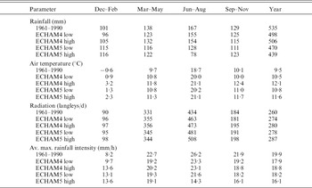
During the reference period, average rainfall amounted to 535 mm/year (Table 3). All future climate scenarios forecast lower rainfall amounts. For the annual averages, the decreases range from 6% (ECHAM4 high) to 18% (ECHAM5 high; Table 3). When considering only spring and summer (March–August), the reductions are from 7 to 9% for ECHAM4 but from 20 to 45% for ECHAM5. ECHAM5 also shows a small increase in rainfall during winter months (December–February).
Seasonal and annual average rainfall, temperature, radiation and average maximum rainfall intensities for investigated climate scenarios

Both climate scenarios predict a temperature increase of 1·0–1·3 and 2·1–2·6°C for low and high climate sensitivity, respectively. Solar radiation is also expected to increase by 5–10%. As rainfall intensity is one of the major drivers of the soil erosion process, it is necessary to know this parameter. Average maximum rainfall intensities during 30 min intervals are shown in Table 3. The highest average annual values occur under current conditions (1961–1990); future climate scenarios deliver lower annual values but show higher 30 min intensities in winter (December–February). Overall, the highest rainfall intensities occur during the summer months (July–August), followed by the spring period (March–May).
WEPP model
For simulation of surface runoff, soil loss within the watershed and sediment yield from the watershed, the WEPP model (Flanagan & Nearing Reference Flanagan and Nearing1995) version 2009.907 was used in combination with its geo-spatial interface (GeoWepp, Renschler Reference Renschler2003). WEPP is a continuous simulation, process-based model that allows the simulation of small watersheds. The geo-spatial interface uses digital geo-referenced information such as digital elevation models, soil and land use maps to derive and prepare valid model input parameters.
The WEPP erosion model computes soil loss along a slope and sediment yield at the end of a hill slope. Interrill and rill erosion processes are considered. Interrill erosion is described as a process of soil detachment by raindrop impact, transport by shallow sheet flow, and sediment delivery to rill channels. Sediment delivery rate to rill flow areas is assumed to be proportional to the product of rainfall intensity and interrill runoff rate. Rill erosion is described as a function of the flow's ability to detach sediment, sediment transport capacity and the existing sediment load in the flow. Net soil detachment in rills occurs when hydraulic shear stress exceeds critical shear stress and when sediment load is less than sediment transport capacity. When sediment load is greater than sediment transport capacity, sediment deposition occurs.
Overland flow processes are conceptualized as a mixture of broad sheet flow occurring in interrill areas and concentrated flow in rill areas. Broad sheet flow on an idealized surface is assumed for overland flow routing and hydrograph development. Overland flow routing procedures include both an analytical solution to the kinematic wave equations and regression equations derived from the kinematic approximation for a range of slope steepness and lengths, friction factors (surface roughness coefficients), soil textural classes and rainfall distributions.
The slope input file required for WEPP was built using digital elevation information from aerial photos. Soil data were collected in the field as well as taken from existing soil maps (Österreichische Bodenkartierung 1995). Soil texture was determined by using a combined wet sieving and sedimentation method (USDA-SCS 1992). Saturated hydraulic conductivity was measured in the field using ring infiltrometer (J. Salvador Munoz, personal communication). For two soil units, saturated hydraulic conductivity was estimated by using the pedotransfer functions in the Rosetta model (Schaap et al. Reference Schaap, Leij and van Genuchten1998).
In WEPP, a modified version of the EPIC (Environmental Policy Integrated Climate) crop growth model is incorporated (Williams et al. Reference Williams, Jones, Kiniry and Spanel1989). It accounts for water and temperature stresses on biomass production and harvested yield. The crop component is designed such that parameters may be adjusted for each different crop and for variation within crop varieties. It is able to predict temporal changes in plant and residue variables such as canopy cover, canopy height and residue or litter cover, which influence the runoff and erosion process. The crop characteristics necessary for hydrologic calculations were chosen from the WEPP crop database. Tillage implements were chosen from WEPP equipment database and if necessary modified for Austrian farming conditions.
As the WEPP model was already validated for the Mistelbach conditions (Klik & Zartl Reference Klik, Zartl, Ascough and Flanagan2001; Klik et al. Reference Klik, Jester, Rauter, Horowitz and Walling2005), soil erodibility parameters for interrill detachment, rill detachment and critical shear were available.
Data analysis
Means and standard deviations are given for simulated data of surface runoff, soil loss and sediment yield. Analysis of variance (ANOVA) was performed to determine significance among treatments using Statistix (1996). All test statistics were evaluated at P=0·05.
RESULTS
Surface runoff
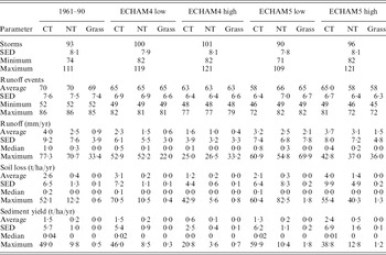
During the reference period 1961–90 an average of 93 rainfall events were recorded per year (Table 4). This number includes all events, regardless of their amount. ECHAM4 generates 100 rainfalls for both scenarios, while ECHAM5 simulates between 90 and 96 events, which is similar to the reference period. Not all of these rainfall events produce surface runoff. Under the current situation, 0·74 of all storms create surface runoff while under future climate scenarios the proportion ranges from 0·58 to 0·72. This decrease of runoff events is significant. More frequent runoff events are simulated for ECHAM5 than for ECHAM4. When soil conservation measures such as NT or grassland are applied, fewer runoff events will occur.
Simulated average number of annual storms and runoff events, average yearly surface runoff, soil loss and sediment yield for the baseline and climate change scenarios

Under conventionally managed field conditions, the simulations predict long-term average surface runoff for the investigated climate scenarios of 1·6–4·0 mm (Table 4). These are very small values and correspond to runoff coefficients of 0·003–0·008. Despite lower annual rainfall amounts, the ECHAM5 scenario produces annual runoff from CT of 3·2–3·7 mm, which is not significantly different than for the baseline period, with up to 95 mm higher precipitation. However, similar runoff occurring in fewer events will increase the runoff amount per event and therefore also its kinetic energy and the erosive force. Under the ECHAM4 scenario, a significant reduction in runoff will occur.
In contrast to CT, the simulations suggest that for most of the future climate scenarios NT practices in the whole watershed would lead to a reduction in annual runoff (1·0–3·1 mm). However, under future scenario ECHAM5, runoff from NT was predicted to increase significantly compared to current conditions. Grassland was predicted to show the highest infiltration rates and therefore lowest runoff (0·4–2·1 mm) for all climate scenarios. Nevertheless, the efficiency of NT and grassland seems to decrease under future scenario ECHAM5, when significant increases in runoff are predicted. This will have implications on water retention in the watershed.
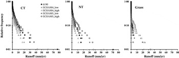
Although the average annual surface runoff is small, there appears to be a high variability of annual values. Maximum annual surface runoff ranges from 25 to 77·3 mm for CT, from 26·5 to 70·7 mm for NT and from 22·0 to 69·9 mm for grassland (Table 4). For CT and NT, the maxima occur under current conditions. ECHAM5 scenarios predict maximum annual runoff similar to current, while ECHAM4 gives much lower results. Figure 2 shows the frequency distribution of annual surface runoff for the investigated land management/use systems and the climate scenarios. This graph illustrates that runoff is low for most of the years. Under CT, the watershed will produce 11·4 mm for baseline conditions and 3·3–10·7 mm for future climate scenarios only once in 10 years. For NT and grassland management options, the corresponding values are 5·5 and 2·0 mm, respectively, for current climatic conditions and 2·6–11·7 and 0–6·9 mm, respectively, for the future. By applying the selected soil conservation measures, annual surface runoff will shift from higher to overall lower values.
Frequency distribution of occurring runoff events.

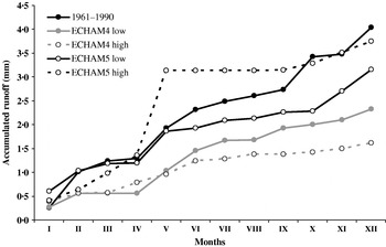
Temporal distribution of surface runoff throughout the year for the different scenarios is shown in Figs 3 and 4. The appearance of surface runoff depends on the ratio of rainfall amount/intensity to infiltration into the soil, and on the antecedent soil moisture conditions (affected by the stage and development of crops as well as by soil cover). The lower rainfall amounts simulated by ECHAM4 scenarios result in lower runoff throughout the whole year for CT (Fig. 3) as well as for NT (Fig. 4) and grass (not shown). This is not the case under the ECHAM5 scenarios. As rainfall also influences crop development, low precipitation can reach critical values which retard growth of vegetation and therefore reduce soil cover. Under ECHAM5, most of the major runoff events (0·47 for CT and 0·55 for NT) are produced in May. Most summer crops are planted between mid-April and mid-May, and appropriate soil moisture is necessary for germination and vegetative crop development. ECHAM5 simulates higher rainfall during winter months but less during the spring (see Table 3). In addition, these spring events still have relatively high maximum intensities. Due to the low rainfall, affecting crop development and therefore soil cover, large portions of the soil surface remain without cover and without physical protection. Low vegetation cover reduces also water losses due to plant transpiration and affects soil water content. Rainfall intensities exceeding the infiltration rate will then produce surface runoff earlier than for soils with good cover.
Temporal distribution of surface runoff for conventional managed conditions (CT) and selected climate scenarios.

Temporal distribution of surface runoff for NT conditions and selected climate scenarios.

Soil erosion and sediment yield
For the reference period, the average annual soil erosion is calculated as between 2·6 t/ha/yr (CT) and 0·01 t/ha/yr (Grass, Table 3). Therefore, CT slightly exceeds the soil loss tolerance level of 2·5 t/ha/yr recommended by the OECD (2001). This value relates to an annual soil loss of c. 0·2 mm which can also be considered as the annual soil formation rate. The average soil erosion rate indicates that within the watershed there are fields which far exceed this level.
For CT, ECHAM4 simulates higher soil loss for low climate sensitivity but lower soil loss for high climate sensitivity. Warmer air temperatures with sufficient rainfall (ECHAM4 low) produce higher above-ground biomass and lead to better coverage of the soil surface, which is also simulated by WEPP. The raindrops will not hit the soil surface directly, but the canopy cover and soil cover; therefore the kinetic energy applied to the soil surface is greatly reduced, leading to a great reduction in soil detachment and soil loss. Insufficient rainfall to fulfil the crop water requirement leads to reduced plant growth, resulting in low vegetation cover. The soil protection systems are able to reduce the already low erosion rates to below 0·2 t/ha/yr.
On average, ECHAM5 scenarios lead to numerically but not statistically higher soil erosion compared to current conditions. The scenario with low climate sensitivity predicts slightly lower soil erosion, while the high sensitivity one predicts a 55% increase. Considering the mean value of 3·07 t/ha/yr, the erosion rate will be above the acceptable soil loss.
For NT, all future scenarios simulate lower erosion rates, except for ECHAM5 high, which predicts a significant increase. Although this scenario estimates a decrease of 65% compared to CT, it simultaneously means an increase of 305% compared to current NT conditions. When the watershed is used as grassland, soil erosion is marginal and this will not change in the future.
Not all detached and eroded soil reaches the watershed outlet. Depending on the topography and size of the watershed, more or less sediment is deposited within it. Under CT, sediment yields of between 1·51 (1961–1990) and 2·38 t/ha/yr (ECHAM5 high) are computed (Table 4). These changes in sediment yield are not significant for ECHAM5. Considering ECHAM4, significantly less sediment will leave the watershed. The results show that 0·47–0·60 of eroded soil will leave the watershed and contribute to off-site effects such as pollution of surface water bodies and siltation of reservoirs, as well as the on-site damage within the watershed due to loss of fertile top soil. Sediment yields from NT in the watershed range from 0·10 (ECHAM4 high) to 0·52 t/ha/yr (ECHAM5 high). Under ECHAM4 a significant reduction in sediment yield can be expected, while under ECHAM5 a significant increase must be considered. Sediment delivery ratio, which expresses the ratio between the sediment yield leaving the watershed to the total amount of soil erosion within the watershed, will then range from 0·37 to 0·70 for NT and from 0·82 to 0·92 for grassland.
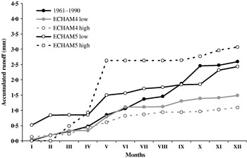
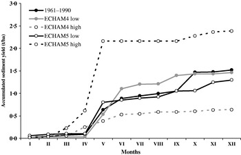
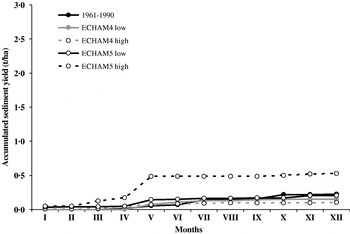
The temporal distribution of the sediment yield clearly shows that the major erosion processes occur in spring (Figs 5 and 6). Considering the current climate, CT and NT produce 0·39 and 0·25, respectively, of the overall annual sediment yield between March and May. For future climate scenarios, the amount of sediment yield generated in spring will be increased to 0·35–0·54 (ECHAM4) and 0·55–0·89 (ECHAM5) for CT, and 0·50–0·55 (ECHAM4) and 0·48–0·83 (ECHAM5) for NT.
Temporal distribution of sediment yield for conventional tilled conditions (CT) and selected climate scenarios.

Temporal distribution of sediment yield for NT conditions and selected climate scenarios.

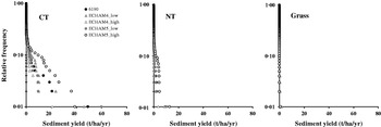
Considering the high variability of erosion throughout the simulated 100 years under current conditions and for CT, a sediment yield higher than 2·6 t/ha/yr will occur once in 10 years (Fig. 7). The values range from 1·2 to 4·2 t/ha/yr for ECHAM4 and from 2·9 to 9·7 t/ha/yr for ECHAM5. Such high sediment yields indicate much higher soil erosion rates within the watershed.
Frequency distribution of soil erosion events.

For NT, the probability of events producing sediment yields of more than 0·3 t/ha/yr under current conditions, and 0·1–0·3 t/ha/yr (ECHAM4) and 0·3–1·5 t/ha/yr (ECHAM5) under future conditions is 0·10 (Fig. 7). For grassland, no sediment yield is simulated for current and ECHAM4 conditions and therefore shows the best protection function once again. No sediments or only marginal amounts leave the watershed under grassland for current as well as future climatic conditions.
DISCUSSION
The results of the present study confirm the significance of just a few months of the year where most of the soil erosion occurs. Under the assumed future climate scenarios, a reduction of 7–18% in annual precipitation is expected. These strong reductions in summer and autumn precipitation far outweigh the predicted precipitation increase in spring. The increase in winter rainfall with respect to soil loss is negligible; it is small in absolute terms and does not affect erosion rates significantly. Peaks in soil loss were identified in spring, during time of seedbed preparation and the early stages of vegetative development of spring planted crops, a period coinciding with heavy rainstorms. Although annual rainfall amounts and amounts of precipitation during these erosion-sensitive periods are likely to be reduced under climate change in the already dry north-eastern part of Austria, soil erosion may not always decrease under these future scenarios. Scholz et al. (Reference Scholz, Quinton and Strauss2008) found similar results for another region in Austria.
Canopy cover, as well as cover of the rill and interrill areas of the soil, is a major factor influencing erosion processes. Future climate scenarios resulted, in most cases, in higher canopy cover, higher leaf area index (LAI) and therefore better plant growth. This implied better soil protection. Simulations for ECHAM4 scenarios calculate reductions in runoff from CT by 42·5–60%, while for ECHAM5 smaller decreases of 7·5–20% are calculated, due to an increase of high intensity rainstorm events. The significant decline of runoff events under ECHAM5, combined with runoff amounts similar to those under current conditions, increase the kinetic energy and the erosive force of the surface runoff. Despite better plant growth, increased soil erosion – especially in periods with low or no soil cover – will be the consequence. In the future, the effectiveness of the selected soil conservation measures will be similar or reduced by 16–53%.
Pruski & Nearing (Reference Pruski and Nearing2002 a) quantified the relationship between a 1% change in precipitation and resulting changes in soil erosion and runoff. Their results suggest increases over current levels of soil erosion from 4 to 96% and increases in runoff from 6 to 100%. Significant increases in precipitation lead to increases in erosion. Under decreasing precipitation the results are more complex, largely due to interactions of plant biomass, runoff and erosion, and either increases or decreases in overall erosion could occur. The same pattern could be observed by the results of the present study. Changes in soil moisture, atmospheric CO2 concentration, temperature and solar radiation each impact biomass production at different levels and will enhance or reduce soil erosion and surface runoff (Fig. 1). Soil cover by vegetation has a higher impact on erosion than on surface runoff. Comparable results were obtained by Nearing et al. (Reference Nearing, Jetten, Baffaut, Cerdan, Couturier, Hernandez, Le Bissonnais, Nichols, Nunes, Renschler, Souchère and van Oost2005) for erosion simulations in two U. S. watersheds and one in Belgium.
The simulations indicate that under CT soil erosion will either decrease by 55% or increase by 56%. Under extreme climatic conditions, average soil loss will reach 4 t/ha/yr and will therefore exceed the level of acceptable soil loss. The use of NT reduces annual soil loss rates to 0·2–1·4 t/ha, which are in the same range or slightly higher than under current conditions. The conversion to grassland minimizes soil losses (>0·03 t/ha/yr). Average soil erosion rates always indicate that much higher soil losses can appear within the watershed, depending on field size, and slope length and steepness. Nevertheless, significantly higher erosion must be expected once in 9 years, exceeding the acceptable soil loss.
Soil erosion is an extreme event process which is mainly driven by rainfall intensity. Rainfall intensity affects soil loss approximately by a power function. Increase in rainfall intensity as indicated by IPCC (2001) is likely to cause an increase in soil loss. These extreme erosion events increase the potential for on-site and off-site damage. Long-term field measurements in Mistelbach on erosion plots showed that 0·95 of the total soil loss was produced by only 0·05 of the storm events (Klik Reference Klik2003).
Other parameters not considered in the present study but which are responsive to climatic variability and climate change are likely to alter the simulated erosion rates further. Increasing CO2 concentrations will enhance plant growth resulting in improved vegetative cover. However, these advantages might be offset by increased water stress for crop plants over the summer, resulting from reduced precipitation amounts.
The methodology used in the present study has some limitations but nevertheless it provides an adequate preliminary assessment of potential effects of climate change on soil erosion and the efficiency of existing soil conservation practices.
CONCLUSION
Only a fertile soil produces healthy crops and a clean groundwater. On a long-term basis, soil erosion by water reduces not only soil productivity but also the storage and filtering function of soils. The main objective of a sustainable soil and land use policy must be the conservation and improvement of the fertility and quality of our soils. Decreasing soil loss by using soil conservation measures represents a major contribution to achieve this goal.
Soil erosion assessments indicate that, despite less rainfall under future climate scenarios, the erosive force of surface runoff may increase and produce higher soil losses from agricultural used fields. Under extreme conditions, average soil erosion can also exceed the soil loss tolerance level. Reductions in rainfall, especially in summer and autumn, can reduce water retention in the landscape and diminish water available for plant production.
Both soil protection measures investigated can be considered as sustainable land use systems under future climatic conditions as they do not exceed the tolerable soil loss on a long-term basis. Nevertheless, on steep slopes the conversion from CT to NT alone will not be sufficient.
For these areas following adaptations of the current erosion control practices are proposed:
• For slopes >6°, crops such as maize, potatoes and sugar beet, which provide relatively low soil cover, should be replaced in the crop rotation by crops or plants which cover the soil most of the year.
• To convey the surface runoff in a non-erodible way, grassed waterways with a width of c. 5 m should be laid out in the valley bottom.
Soil is a limited resource and represents the main basis for food production for future generations. Therefore, soil protection must be a high priority. Reduced soil tillage/management systems and grassland – with small adaptations – are effective and sustainable soil use systems under future climate conditions as well as the present conditions because they maintain and improve the different functions of the soil. However, the results obtained in the present study suggest that there is a potential for climate change to increase soil erosion rates in the north-eastern part of Austria unless conservation measures are taken to offset this.
This study was partly funded by the Austrian Federal Ministry of Agriculture, Forestry, Environment and Water Management, the Austrian Federal Ministry of Science and Research and the Austrian Hail Insurance.