1. Introduction
1.1 Local coefficients
In previous work, the authors introduced an instanton homology,  $I^{\sharp }(K)$, for knots and links
 $K \subset S^{3}$. It was constructed as the Morse homology of a Chern–Simons functional whose critical points correspond to certain
 $\mathop {{SU}}\nolimits (2)$ representations of the fundamental group of the link complement. A variant
 $J^{\sharp }(K)$ was introduced in [Reference Kronheimer and MrowkaKM19b], and was defined similarly, but with
 $\mathop {{SO}}(3)$ in place of
 $\mathop {{SU}}\nolimits (2)$. The coefficient ring in the present paper will have characteristic
 $2$ and, when this is the case, both
 $I^{\sharp }(K)$ and
 $J^{\sharp }(K)$ can be defined for webs (embedded trivalent graphs) rather than only for links. One of the main results [Reference Kronheimer and MrowkaKM12] concerning
 $I^{\sharp }(K)$ is the existence of a spectral sequence abutting to
 $I^{\sharp }(K)$ and having
 $E_{2}$ page isomorphic to Khovanov homology:
 \begin{equation} \mathop{\mathsf{Kh}}\nolimits(\bar{K}) \implies I^{\sharp}(K). \end{equation}
(The notation  $\bar {K}$ denotes the mirror image of
 $K$ and it appears here only because some of the traditional orientation conventions differ.)
In this paper  $K$ will nearly always be a knot or link: trivalent spatial graphs appear only in an auxiliary role. We focus on a variant of
 $I^{\sharp }(K)$ obtained by introducing a system of local coefficients on the relevant configuration space of connections,
 $\mathcal {B}^{\sharp }(K)$. In doing so, we build on two earlier papers. First, in [Reference Kronheimer and MrowkaKM13], the authors introduced a local coefficient system, denoted here by
 $\Gamma _{o}$. It is defined as the pull-back of a local system on
 $S^{1}$ via a map
 \[ h_{o} : \mathcal{B}^{\sharp}(K) \to S^{1}, \]
which in turn is defined using the holonomy of the connection along  $K$. In characteristic
 $0$, a spectral sequence similar to (1) was established abutting to
 $I^{\sharp }(K ; \Gamma _{o})$, where the role of
 $\mathop {\mathsf {Kh}}\nolimits (\bar {K})$ is taken by Lee homology, a certain deformation of Khovanov homology introduced in [Reference LeeLee03, Reference LeeLee05]. The local system
 $\Gamma _{o}$ is a system of free modules of rank
 $1$ over the ring
 $\mathbb{Q}[\mathbb{Z}] = \mathbb{Q}[u,u^{-1}]$, though we will see later how it may be defined also in characteristic
 $2$.
Second, in [Reference Kronheimer and MrowkaKM19a], a local system  $\Gamma _{\theta }$ was introduced. Its construction is similar to
 $\Gamma _{o}$, but makes use of the holonomy along the three edges of an auxiliary theta graph to define a map
 \[ h_{\theta} : \mathcal{B}^{\sharp}(K) \to S^{1} \times S^{1} \times S^{1}. \]
The result is a system of free rank-1 modules over the ring
 \begin{equation} \mathbb{F}_{2}[\mathbb{Z}^{3}] = \mathbb{F}_{2}[T_{1}^{{\pm} 1}, T_{2}^{{\pm} 1}, T_{3}^{{\pm} 1}], \end{equation}
where  $\mathbb{F}_{2}$ is the field of two elements.
In this paper, we introduce a local system  $\Gamma$ that generalizes both
 $\Gamma _{o}$ (in its characteristic-
 $2$ version) and
 $\Gamma _{\theta }$. It is a local system of rank-1 modules over a ring of Laurent series in four variables:
 \begin{equation} \mathcal{R} = \mathbb{F}_{2} [T_{0}^{{\pm} 1}, T_{1}^{{\pm} 1}, T_{2}^{{\pm} 1}, T_{3}^{{\pm} 1}]. \end{equation}
The local system  $\Gamma _{o}$ can be recovered as a specialization of
 $\Gamma$ by setting
 $T_{i}=1$ for
 $i=1,2,3$, while the local system
 $\Gamma _{\theta }$ is obtained by setting
 $T_{0}=1$.
1.2 A spectral sequence from  $F_{5}$ homology

Lee homology, mentioned above, is a member of a larger family of deformations of Khovanov homology which are classified in [Reference Bar-NatanBar05] and [Reference KhovanovKho06]. In the language and notation of [Reference KhovanovKho06], these are link homologies  $\mathsf {H}(K ; F)$ arising from rank-2 Frobenius systems
 $F$. Among these, one that is shown to be universal in a particular sense arises from a Frobenius system over the ring
 $\mathbb{Z}[h,t]$. We will work exclusively in characteristic
 $2$ and in place of Khovanov's
 $\mathbb{Z}[h,t]$ we introduce the ring
 \[ R_{5} = \mathbb{F}_{2}[h,t] \]
and a corresponding Frobenius system  $F_{5}$ whose underlying ring is
 $R_{5}[X]/(X^{2} + h X +t )$ and whose comultiplication is given by
 \begin{align*} \Delta: 1&\mapsto 1\otimes X + X\otimes 1 + h(1\otimes 1), \\ \Delta: X&\mapsto X\otimes X + t(1\otimes 1). \end{align*}
(The subscript  $5$ in
 $R_{5}$ and
 $F_{5}$ follows the naming convention in [Reference KhovanovKho06].) The corresponding link homology is denoted here by
 $\mathsf {H}(K; F_{5})$. It is a module over
 $R_{5}$ and is equal to
 $F_{5}$ when
 $K$ is the unknot. The first topic of this paper is the construction of an instanton homology
 $I^{\sharp }(K ; \Gamma )$ corresponding to the local system of
 $\mathcal {R}$-modules
 $\Gamma$ described above, and the construction of the following spectral sequence.
Theorem 1.1 For a knot or link in  $\mathbb{R}^{3}$, there is a spectral sequence of
 $\mathcal {R}$-modules from the
 $F_{5}$ homology (in characteristic
 $2$) to the instanton homology with local coefficients:
 \begin{equation} \mathsf{H}(\bar{K} ; F_{5} \otimes_{r} \mathcal{R} ) \implies I^{\sharp}(K; \Gamma). \end{equation}
Here the base-change homomorphism  $r: R_{5}\to \mathcal {R}$ is given by
 \begin{align*} r(h) &= P, \\ r(t) &= Q, \end{align*}
where
 \begin{equation} P = T_{1}T_{2}T_{3} + T_{1}T_{2}^{{-}1}T_{3}^{{-}1} + T_{2}T_{3}^{{-}1}T_{1}^{{-}1} + T_{3}T_{1}^{{-}1}T_{2}^{{-}1} \end{equation}
and
 \[ Q = \sum_{j=0}^{3} (T^{2}_{j} + T_{j}^{{-}2} ). \]
Remark Because  $\mathcal {R}$ is a free module over
 $R_{5}$, one can take the tensor product outside and rewrite the spectral sequence as
 \[ \mathsf{H}(\bar{K} ; F_{5} ) \otimes_{r} \mathcal{R} \implies I^{\sharp}(K; \Gamma). \]
1.3 Bar-Natan homology
By base change of the coefficient ring via a further ring homomorphism  $\sigma :\mathcal {R}\to \mathcal {S}$, one obtains specializations of the spectral sequence (4):
 \begin{equation} \mathsf{H}(\bar{K} ; F_{5} \otimes_{\sigma\circ r} \mathcal{S} ) \implies I^{\sharp}(K;\, \Gamma\otimes_{\sigma}\mathcal{S}). \end{equation}
As a particular case of this construction, we can obtain a spectral sequence from the graded Bar-Natan link homology  $\mathop {\mathsf {BN}}\nolimits (K)$ introduced in [Reference Bar-NatanBar05]. There is in fact some freedom in the construction of such a spectral sequence. To explain this, recall that in the context of [Reference KhovanovKho06] and [Reference Bar-NatanBar05], the homology
 $\mathop {\mathsf {BN}}\nolimits (K)$ arises from the Frobenius system
 $F_{5}$ by a base change
 \[ \tau_{{bn}} : R_{5} \to S_{{bn}}, \]
where  $S_{{bn}}=\mathbb{F}_{2}[h]$ and
 $\tau _{{bn}}$ is the homomorphism sending
 $t$ to
 $0$. We write
 $F_{{bn}} = F_{5}\otimes _{\tau _{{bn}}} S_{{bn}}$ for the corresponding Frobenius system, so that
 $\mathop {\mathsf {BN}}\nolimits (K)$ is short-hand for
 $\mathsf {H}(K; F_{{bn}})$. Specifically, the underlying algebra of the Frobenius system
 $F_{{bn}}$ is
 \[ S_{{bn}}[X] / (X^{2} + hX) \]
and the comultiplication is
 \begin{align*} \Delta: 1&\mapsto 1\otimes X + X\otimes 1 + h (1\otimes 1), \\ \Delta: X&\mapsto X\otimes X. \end{align*}
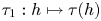
At the expense of working over a larger ring than  $S_{{bn}}$, we can equivalently consider any ring homomorphism
 \[ \tau : R_{5} \to S \]
with the following two properties:
(i) the polynomial
$x^{2} + \tau (h) x + \tau (t)$ factorizes:
(7)\begin{equation} x^{2} + \tau(h) x + \tau(t) = (x+a)(x+a') \quad (a,a' \in S); \end{equation}(ii) the ring
$S$ is a free module over $S_{{bn}}=\mathbb{F}_{2}[h]$ via the homomorphism $\tau _{1}: h\mapsto \tau (h)$.



When factorization occurs, the Frobenius system  $F_{5}\otimes _{\tau } S$ can be described in terms of a new generator
 $M = X+a'$ and the algebra becomes
 \[ S[M] / (M^{2} + \tau(h) M). \]
Thus, the ‘ $t$’ term disappears from the characteristic polynomial of
 $M$. The comultiplication is
 \begin{align*} \Delta: 1 &\mapsto 1\otimes M + M\otimes 1 + \tau(h)(1\otimes 1), \\ \Delta: M &\mapsto M\otimes M. \end{align*}
When condition (ii) holds, an application of the universal coefficient theorem shows that
 \[ \mathsf{H} (K ; F_{5}\otimes_{\tau} S ) \cong \mathop{\mathsf{BN}}\nolimits(K)\otimes_{\tau_{1}} S. \]
That is, the link homology arising from the Frobenius system  $F_{5}\otimes _{\tau } S$ is isomorphic to the graded Bar-Natan homology with the coefficients extended trivially from
 $S_{{bn}}=\mathbb{F}_{2}[h]$ to
 $S$.
With this in mind, we return to the instanton homology  $I^{\sharp }(K; \Gamma )$ as a module over
 $\mathcal {R}$. Suppose that we find a ring
 $\mathcal {S}$ and a base change
 \[ \sigma: \mathcal{R} \to \mathcal{S} \]
such that the counterparts of the two conditions above hold:
(i) the polynomial
$x^{2} + \sigma (P) x + \sigma (Q)$ factorizes in $\mathcal {S}[x]$:
(8)\begin{equation} x^{2} + \sigma(P) x + \sigma(Q) = (x+A)(x+A') \quad (A,A' \in \mathcal{S}); \end{equation}(ii) the ring
$\mathcal {S}$ is a free module over $S_{{bn}}=\mathbb{F}_{2}[h]$ via the homomorphism $r_{1}: h\mapsto \sigma (P)$.




If we examine the spectral sequence (6) under these conditions, we see from the observations above that the link homology that appears on the left (the  $E_{2}$ page of the spectral sequence) is isomorphic to graded Bar-Natan homology with a trivial extension of coefficients:
 \[ \mathsf{H}(\bar{K} ; F_{5} \otimes_{\sigma\circ r} \mathcal{S} ) \cong \mathop{\mathsf{BN}}\nolimits(\bar{K})\otimes_{r_{1}} \mathcal{S}. \]
In this way we obtain a spectral sequence from 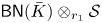 $\mathop {\mathsf {BN}}\nolimits (\bar {K})\otimes _{r_{1}}\mathcal {S}$ to
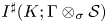 $I^{\sharp }(K; \Gamma \otimes _{\sigma } \mathcal {S})$.
To be specific about a base change that realizes the requirements (i) and (ii), we can consider
 \begin{equation} \sigma_{{bn}} : \mathcal{R} \to \mathcal{S}_{\mathop{\mathsf{BN}}\nolimits}, \end{equation}
where  $\mathcal {S}_{\mathop {\mathsf {BN}}\nolimits }= \mathbb{F}_{2}[T_{1}^{\pm 1} , T_{2}^{\pm 1}, T_{3}^{\pm 1}]$ is a ring of Laurent series in three variables and
 \begin{equation} \begin{aligned} \sigma_{{bn}}(T_{0}) & =T_{1}, \\ \sigma_{{bn}}(T_{i}) & = T_{i} ,\quad i=1,2,3. \end{aligned} \end{equation}
We can write
 \begin{align*} \sigma_{{bn}}(P) &= A + A', \\ \sigma_{{bn}}(Q) &= AA', \end{align*}
where
 \begin{equation} \begin{aligned} A & = T_{1}\big(T_{2}T_{3} + T_{2}^{{-}1}T_{3}^{{-}1}\big),\\ A' & = T_{1}^{{-}1}\big(T_{2}^{{-}1}T_{3} + T_{2}T_{3}^{{-}1}\big),\\ \end{aligned} \end{equation}
so that the factorization (i) indeed occurs. Putting this together, we have the following statement.
Corollary 1.2 There is a spectral sequence of modules over the Laurent series ring  $\mathcal {S}_{\mathop {\mathsf {BN}}\nolimits }$ in three variables from the graded Bar-Natan homology in characteristic
 $2$
 \[ \mathop{\mathsf{BN}}\nolimits(\bar{K}) \otimes_{r_{1}} \mathcal{S}_{\mathop{\mathsf{BN}}\nolimits} \implies I^{\sharp}(K ; \Gamma_{\mathop{\mathsf{BN}}\nolimits}) \]
to the instanton homology group with coefficients in the local system  $\Gamma _{\mathop {\mathsf {BN}}\nolimits }= \Gamma \otimes _{\sigma _{{bn}}}\mathcal {S}_{\mathop {\mathsf {BN}}\nolimits }$, where the base change
 $\sigma _{bn}$ is given by (10).
We shall also introduce a reduced companion of the instanton homology group  $I^{\sharp }(K ; \Gamma _{\mathop {\mathsf {BN}}\nolimits })$, which we shall denote by
 $I^{\natural }(K; \Gamma _{\mathop {\mathsf {BN}}\nolimits })$. The spectral sequence of Corollary 1.2 has a reduced companion whose
 $E_{2}$ page is the reduced Bar-Natan homology. Such a reduced instanton homology group can be defined using any local system of the form
 $\Gamma \otimes _{\sigma } \mathcal {S}$ provided that the base change
 $\sigma$ satisfies
 $\sigma (T_{0})=\sigma (T_{1})$. In particular, there is no reduced version of
 $I^{\sharp }(K;\Gamma )$ itself. Correspondingly, there is no reduced version of the link homology
 $\mathsf {H}(K; F_{5})$ without first making a base change so that the polynomial
 $x^{2} + h x + t$ factorizes.
There are smaller rings  $\mathcal {S}$ that can be used in place of our
 $\mathcal {S}_{\mathop {\mathsf {BN}}\nolimits }$ in formulating this corollary. Notice that a sufficient condition for the factorization (i) to occur is that
 $\sigma (Q)=0$. So as another particular example we can take
 \[ \mathcal{S}=\mathbb{F}_{2}\big[T,T^{{-}1}\big] \]
and
 \[ \sigma(T_{i})= \begin{cases} 1, & i=0,1,\\ T, & i=2,3. \end{cases} \]
Then  $\sigma (P) = T^{2} + T^{-2}$ and
 $\sigma (Q)=0$. The homomorphism
 $r_{1}:S_{{bn}}\to \mathcal {S}$ in this case is therefore given by
 \[ r_{1}(h) = T^{2} + T^{{-}2}. \]
Example For the right-handed trefoil  $K$, the reduced Bar-Natan homology
 $\widetilde {\mathop {\mathsf {BN}}\nolimits }(\bar {K})$ with mod-2 coefficients is
 $S_{{bn}} \oplus (S_{{bn}}/\langle h \rangle )$ as a module over the polynomial ring
 $S_{{bn}}=\mathbb{F}_{2}[h]$. The reduced instanton homology
 $I^{\natural }(K ; \Gamma _{\sigma })$ over the ring
 $\mathcal {S}=\mathbb{F}_{2}[T, T^{-1}]$ in this case is
 $\mathcal {S} \oplus (\mathcal {S}/\langle T^{2}+T^{-2} \rangle )$. The latter computation is given in [Reference Kronheimer and MrowkaKM19c].
There is also a filtered (as opposed to graded) version of Bar-Natan homology, which we denote by  $\mathop {\mathsf {fBN}}\nolimits (K)$. It is obtained via further specialization from
 $(R_{5}, F_{5})$ by setting
 $t=0$ and
 $h=1$. The result is a finite-dimensional
 $\mathbb{F}_{2}$ vector space. For an instanton companion, we may pass to
 $\mathbb{F}_{4}$, the field of four elements, or any extension of
 $\mathbb{F}_{2}$ in which there is a solution
 $\zeta$ for the equation
 $T^{2}+T^{-2}=1$. We define
 \begin{equation} \begin{aligned} & {\sigma}_{{fbn}} : \mathcal{R} \to\mathbb{F}_{4},\\ & T_{i} \mapsto \begin{cases} 1, & i=0,1,\\ \zeta, & i=2,3, \end{cases} \end{aligned} \end{equation}
so that  $Q\mapsto 0$ and
 $P \mapsto 1$. There is a corresponding local system of one-dimensional
 $\mathbb{F}_{4}$-vector spaces,
 \[ \Gamma_{\mathop{\mathsf{fBN}}\nolimits} = \Gamma\otimes_{\sigma_{{fbn}}} \mathbb{F}_{4}. \]
We then have the following result.
Corollary 1.3 For a knot or link  $K$, let
 $\mathop {\mathsf {fBN}}\nolimits (K)$ denote the filtered Bar-Natan homology over
 $\mathbb{F}_{2}$. Then there is a spectral sequence of vector spaces over
 $\mathbb{F}_{4}$,
 \[ \mathop{\mathsf{fBN}}\nolimits(\bar{K})\otimes \mathbb{F}_{4} \implies I^{\sharp}(K ; \Gamma_{\mathop{\mathsf{fBN}}\nolimits}), \]
where  $\Gamma _{\mathop {\mathsf {fBN}}\nolimits }$ is the local system of
 $\kern0.05em \mathbb{F}_{4}$ vector spaces described above.
Since  $I^{\sharp }(K;\Gamma )$ can be defined for trivalent spatial graphs as well as knots and links, it would be interesting to know whether there exist corresponding generalizations of the spectral sequence (4) or any of its specializations, where the link homologies
 $\mathsf {H}(K; F_{5})$,
 $\mathop {\mathsf {BN}}\nolimits (K)$ or
 $\mathop {\mathsf {fBN}}\nolimits (K)$ are replaced by combinatorial invariants of spatial graphs. Note however that
 $I^{\sharp }(K;\Gamma )$ is a torsion
 $\mathcal {R}$-module when
 $K$ has vertices (it is annihilated by
 $P$) and
 $I^{\sharp }(K;\Gamma _{\mathop {\mathsf {fBN}}\nolimits })$ is zero. A different connection between Bar-Natan homology and gauge theory, this time with Seiberg–Witten theory, has been described by Lin [Reference LinLin19].
2. The construction of $I^{\sharp }(K ; \Gamma )$

In this section we describe the construction of the local system  $\Gamma$ and the instanton homology
 $I^{\sharp }(K ; \Gamma )$. We will lean heavily on the expositions in the earlier papers [Reference Kronheimer and MrowkaKM19a] and [Reference Kronheimer and MrowkaKM19b], which were concerned with two different specializations for
 $\Gamma$.
2.1 Instanton homology with constant coefficients
A trivalent graph, or web,  $K$ in a closed oriented
 $3$-manifold
 $Y$ gives rise to an orbifold, which we will simply denote by
 $(Y,K)$. The isotropy groups are taken to be
 $\mathbb{Z}/2$ along edges of
 $K$ and
 $\mathbb{Z}/2 \times \mathbb{Z}/2$ at the vertices. We refer to such a special orbifold as a bifold and we consider orbifold
 $\mathop {{SO}}(3)$ bundles (or bifold bundles)
 $E$ over
 $(Y,K)$ requiring that the local isotropy groups of the orbifold act effectively on the
 $\mathop {{SO}}(3)$ fibers. Marking data on
 $(Y,K)$ consists of an open set
 $U_{\mu }$ and a bifold bundle
 $E_{\mu }\to U_{\mu } {\setminus} K$; a bifold connection is marked by
 $\mu$ if an isomorphism
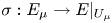 $\sigma : E_{\mu } \to E|_{U_{\mu }}$ is given. An isomorphism
 $\tau$ between
 $\mu$-marked bundles with connection,
 $(E,A,\sigma )$,
 $(E',A',\sigma ')$, is an isomorphism of bifold bundles-with-connection such that the automorphism
 $\sigma ^{-1}\tau \sigma ' : E_{\mu }\to E_{\mu }$ lifts to the determinant-1 gauge group. We write
 \[ \mathcal{B}(Y, K ; \mu) \]
for the space of isomorphism classes of  $\mu$-marked bifold bundles with connection.
The marking data  $\mu$ is strong if the automorphism group of every flat
 $\mu$-marked bifold connection is trivial. A sufficient condition is that
 $U_{\mu }$ contains a vertex of
 $K$ and in this case there are indeed no connections with non-trivial stabilizer even in
 $\mathcal {B}(Y, K; \mu )$. With coefficients in the field
 $\mathbb{F}_{2}$ of two elements, one can construct an
 $\mathop {{SO}}(3)$ instanton homology group
 \[ J((Y,K) ; \mu) \]
for any bifold with strong marking data. The generators of the complex from which this instanton homology is computed correspond to critical points of a perturbed Chern–Simons functional on  $\mathcal {B}(Y, K ; \mu )$. We may omit
 $Y$ from our notation for both
 $J$ and
 $\mathcal {B}$ when
 $Y$ is understood (which is often the case when
 $Y$ is
 $S^{3}$).
Consider next a framed base point  $y_{0} \in Y$ with standard neighborhood
 $B(y_{0}) \cong B^{3}$. We write
 $Y^{o}$ for the complement of this standard neighborhood:
 \[ Y^{o} = Y {\setminus} B(y_{0}). \]
Given a web
 \[ K \subset Y^{o}, \]
we may form a new web as a split union
 \begin{equation} K^{\sharp} = K \cup \theta, \end{equation}
where  $\theta \subset B(y_{0})$ is a standard theta graph (three edges and two vertices) contained in the ball. We may then define
 \begin{equation} J^{\sharp}(K) = J((Y, K^{\sharp}); \mu_{\theta}), \end{equation}
where the marking data  $\mu _{\theta }$ consists of the ball
 $U_{\theta } = B(y_{0})$ containing
 $\theta$, with
 $E_{\theta }$ the unique trivial bundle on
 $B^{3}{\setminus} \theta$. The group
 $J^{\sharp }(K)$ was defined first in [Reference Kronheimer and MrowkaKM19b], though the description in that paper was a slight variant of this one. The description we have just given is from [Reference Kronheimer and MrowkaKM19a], where the equivalence of the two descriptions is also proved.
In this paper, we will be almost exclusively concerned with the case that the marking region  $U_{\mu }$ is not just the ball
 $B(y_{0})$ but is instead the whole of
 $Y$. The distinguished
 $\mathop {{SO}}(3)$ bundle
 $E_{\mu }$ on
 $Y{\setminus} K^{\sharp }$ may in general have non-zero Stiefel–Whitney class
 \[ w_{2}(E_{\mu}) \in H^{2} ( Y{\setminus} K^{\sharp} ; \mathbb{Z}/2). \]
We take this class to be represented by  $\omega \subset Y$, which is a codimension-2 submanifold with boundary. We make the following assumptions on
 $\omega$:
–
$\omega$ is (the interior of) a union of circles and arcs with end points on $K$;–
$\omega$ is disjoint from the ball $B(y_{0})$ which contains $\theta$.


We require that  $\omega$ represents
 $w_{2}(E_{\mu })$, in the sense that
 \[ w_{2}(E_{\mu}) = \mathop{PD}\big[\omega \cap (Y{\setminus} K^{\sharp})\big]. \]
Having chosen  $\omega$, we shall trivialize
 $E_{\mu }$ on the complement of
 $\omega$, so that the obstruction to extending the trivialization across each component of
 $\omega$ is non-zero. We use this trivialization to give a lift of
 $E_{\mu }$ to an
 $\mathop {{SU}}\nolimits (2)$ bundle on the complement of
 $\omega$.
Let us write  $\mu _{\omega }$ for the marking data obtained in this way from a 1-manifold
 $\omega \subset Y {\setminus} K^{\sharp }$.
Definition 2.1 Using the marking data  $E_{\mu }$ as above, whose Stiefel–Whitney class is dual to
 $\omega \subset Y{\setminus} K$, we write
 \begin{equation} I^{\sharp}(K)_{\omega} = J((Y, K^{\sharp}); \mu_{\omega}) \end{equation}
for the corresponding instanton homology of the web  $K\subset Y^{o}$. We also write
 \begin{equation} \mathcal{B}^{\sharp}(K)_{\omega} = \mathcal{B}\big((Y, K^{\sharp}) ; \mu_{\omega}\big) \end{equation}
for the corresponding configuration space of connections. When  $\omega$ is empty, we simply omit it from our notation and write
 $I^{\sharp }(K)$.
When  $K$ is a knot or link, this variant coincides with the mod-2 version of the invariant
 $I^{\sharp }(K)_{\omega }$ as introduced in [Reference Kronheimer and MrowkaKM12] (though in that paper the coefficient ring was
 $\mathbb{Z}$). As with
 $J^{\sharp }$, the definition we have presented here is slightly different from the earlier one: the difference is the use of the graph
 $\theta$ in place of the Hopf link that was used in [Reference Kronheimer and MrowkaKM12]. But the two definitions give isomorphic homology groups, by the arguments from [Reference Kronheimer and MrowkaKM19a].
Because the marking data is all of  $Y$, the gauge theory which underlies this instanton homology is essentially an
 $\mathop {{SU}}\nolimits (2)$ gauge theory. In particular, we have the following identification.
Lemma 2.2 The space  $\mathcal {B}^{\sharp }(K)_{\omega }$ parametrizes equivalence classes of data of the following sort:
– an
$\mathop {{SU}}\nolimits (2)$ bundle $\hat {E}$ over $Y{\setminus} (K^{\sharp } \cup \omega )$;– an
$\mathop {{SU}}\nolimits (2)$ connection $\hat {A}$ in $\hat {E}$, subject to the restrictions;– the associated
$\mathop {{SO}}(3)$ connection $A$ in the adjoint bundle of $\hat {E}$ is the restriction to $Y{\setminus} (K^{\sharp } \cup \omega )$ of a bifold bundle on the bifold $(Y, K^{\sharp })$;– the limiting holonomy of
$\hat {A}$ on small circles linking $\omega$ is $-1$.


2.2 The local system
We begin with some motivation of our construction. If  $\pi$ denotes the fundamental group of the configuration space
 $\mathcal {B}^{\sharp }(K)_{\omega }$, then there is a tautological local system over
 $\mathcal {B}^{\sharp }(K)_{\omega }$ whose fiber at each point is a free rank-1 module for the group ring
 $\mathbb{F}_{2}[\pi ]$. It can be realized by defining its fiber at
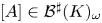 $[A] \in \mathcal {B}^{\sharp }(K)_{\omega }$ to be the vector space of
 $\mathbb{F}_{2}$-valued functions with finite support on the fiber of the universal cover
 $\tilde {\mathcal {B}}^{\sharp }(K)_{\omega } \to \mathcal {B}^{\sharp }(K)_{\omega }$. Given any choice of homomorphism
 \[ \epsilon: \pi \to G, \]
there is a corresponding local system  $\Gamma _{\epsilon }$ of
 $\mathbb{F}_{2}[G]$ modules. Our instanton homology is
 $\mathbb{Z}/2$ graded, not
 $\mathbb{Z}$ graded, because of non-trivial spectral flow, and there is an infinite cyclic cover of
 $\mathcal {B}^{\sharp }(K)$ on which the spectral flow is trivial. Let
 \[ \pi' \subset \pi \]
be the fundamental group of this infinite cyclic cover. The instanton homology groups are essentially unchanged in passing to the cover (the homology becomes  $\mathbb{Z}$ graded and 2-periodic, rather than
 $\mathbb{Z}/2$ graded). Up to isomorphism, the instanton homology groups with coefficients in the local system
 $\Gamma _{\epsilon }$ will therefore depend on the homomorphism
 $\epsilon$ only through the restriction of
 $\epsilon$ to
 $\pi '$.
Although we shall not need a proof, the fundamental group  $\pi$ is a free abelian group of rank
 $5$ when
 $K$ is a knot and
 $\omega$ is empty. It follows in this case that
 $\pi '$ has rank
 $4$ and we will therefore capture the most general local system if we construct a homomorphism
 \[ \pi \to \mathbb{Z}^{4} \]
which is injective on the subgroup  $\pi ' \subset \pi$.
The construction described in [Reference Kronheimer and MrowkaKM19a] arises from a map
 \[ \pi \to \mathbb{Z}^{3} \]
presented in terms of an explicit map
 \[ \big(h_{1}, h_{2}, h_{3}\big): \mathcal{B}^{\sharp}(K)_{\omega} \to S^{1} \times S^{1} \times S^{1} \]
and this leads to the local system  $\Gamma _{\theta }$ of free rank-1 modules over
 $\mathbb{F}_{2}[\mathbb{Z}^{3}]$ as described at (2) in the introduction. To recall this briefly from [Reference Kronheimer and MrowkaKM19a], the marking data
 $\mu _{\omega }$ means that our gauge theory has structure group
 $\mathop {{SU}}\nolimits (2)$ and, at the two vertices of
 $\theta$, the structure group of the two fibers
 $E_{+}$ and
 $E_{-}$ is reduced to the center
 $\{\pm 1\}$. Along each edge of
 $\theta$, the structure group is reduced to
 $S^{1}$. The holonomy along each edge therefore gives a well-defined element of
 \begin{equation} S^{1} / \{{\pm} 1\} \cong \mathbb{R}/\mathbb{Z}. \end{equation}
Applied to the three edges of  $\theta$ in turn, one obtains the three components
 $h_{1}$,
 $h_{2}$,
 $h_{3}$. (The notation for
 $\Gamma _{\theta }$ was simply
 $\Gamma$ in [Reference Kronheimer and MrowkaKM19a].)
When  $\omega$ has no end points (so is disjoint from
 $K$), a very similar construction from [Reference Kronheimer and MrowkaKM13] can be adapted to define a map
 \begin{equation} h_{0} : \mathcal{B}^{\sharp}(K)_{\omega} \to S^{1}. \end{equation}
To describe this, consider first the case that  $K$ is a knot. Choose a framing
 $\tau$ for
 $K$ so as to have well-defined push-off. As explained in [Reference Kronheimer and MrowkaKM11], the framing allows us to interpret the orbifold connection
 $[A]$ as giving rise to a well-defined connection over the knot
 $K$ itself, carried by a bundle with an involution
 $g$ coming from the orbifold structure. Because of the action of
 $g$, the adjoint bundle decomposes as a sum
 \[ \xi \oplus \eta, \]
where  $\xi$ is a real line bundle on
 $K$ and
 $\eta$ is a 2-plane bundle. The marking data allows us to identify the orientation bundle of the knot
 $K$ with the orientation bundles of both
 $\xi$ and
 $\eta$, so the connection in the 2-plane bundle
 $\eta$ has a well-defined circle-valued holonomy along
 $K$. The holonomy of
 $\eta$ around
 $K$ is the definition of
 $h_{0}$ above. If
 $K$ is a link rather than a knot, we multiply the holonomies along all the components.
Combining the two previous constructions, we now have a map
 \begin{equation} \big(h_{0}, h_{1}, h_{2}, h_{3}\big) : \mathcal{B}^{\sharp}(K)_{\omega} \to \mathbb{R}^{4}/\mathbb{Z}^{4} \end{equation}
whenever  $\omega$ has no boundary points. In the case that
 $\omega$ has boundary on
 $K$, the component
 $h_{0}$ must be omitted. As in [Reference Kronheimer and MrowkaKM11], we use an explicit description of the corresponding local system that depends on the maps
 $h_{i}$ but does not depend on a choice of base point in
 $\mathcal {B}^{\sharp }(K)_{\omega }$. We write
 \[ \mathcal{R} = \mathbb{F}_{2}[ \mathbb{Z}^{4}] \]
and regard this as a subring of  $\mathbb{F}_{2}[\mathbb{R}^{4}]$. For each
 $\mu \in \mathbb{R}^{4}$, we have the rank-1
 $\mathcal {R}$-module
 \begin{align*} \Gamma|_{\mu} &= T_{0}^{\mu_{0}} T_{1}^{\mu_{1}} T_{2}^{\mu_{2}} T_{3}^{\mu_{3}} \mathcal{R} \\ &\subset \mathbb{F}[\mathbb{R}^{4}] \end{align*}
and these form a local system over the torus  $\mathbb{R}^{4}/\mathbb{Z}^{4}$. Pulling this back by the map (19), we obtain our local system
 $\Gamma$ over
 $\mathcal {B}^{\sharp }(K)_{\omega }$.
We summarize these constructions as follows.
Notation 2.3 Let  $K \subset Y^{o}$ be a link, let
 $K^{\sharp } = K \cup \theta$ and let
 $\omega \subset Y$ be a 1-manifold without boundary, disjoint from the ball containing
 $\theta$. Let
 $\mathcal {B}^{\sharp }(K)_{\omega }$ be the associated space of connections. On
 $\mathcal {B}^{\sharp }(K)_{\omega }$, we have a local system
 $\Gamma$ of (free, rank-1) modules over
 \[ \mathcal{R}=\mathbb{F}_{2}[\mathbb{Z}^{4}]. \]
For any base change  $\sigma :\mathcal {R}\to \mathcal {S}$, there is a corresponding system of
 $\mathcal {S}$-modules,
 \[ \Gamma_{\sigma} = \Gamma\otimes_{\sigma}\mathcal{S}. \]
If  $\sigma (T_{0})=1$, then the map
 $h_{0} : \mathcal {B}^{\sharp }(K)_{\omega } \to S^{1}$ is not required in the construction of the local system, and in this case we can form the local system
 $\Gamma _{\sigma }$ more generally, when
 $\omega$ is allowed to be a manifold with boundary with end points on
 $K$.
Remarks (i) In the case that  $\omega$ has boundary and
 $\sigma (T_{0})=1$, our notation for the local system
 $\Gamma _{\sigma }$ involves a slight abuse of notation, since we can no longer write it as
 $\Gamma \otimes _{\sigma } \mathcal {S}$. (The local system
 $\Gamma$ is not defined in this case.) It should more properly be defined as
 $\Gamma _{\theta }\otimes _{\bar {\sigma }} \mathcal {S}$, where
 $\bar {\sigma } : \mathbb{F}_{2}[\mathbb{Z}^{3}] \to \mathcal {S}$ is the map through which
 $\sigma$ factors.
(ii) The definition of  $h_{0}$ above makes use of a framing
 $\tau$ for the knot (or for each component of the link). If the framing
 $\tau$ is changed by
 $1$, then
 $h_{0}$ changes to
 $h_{0} + 1/2$. (See [Reference Kronheimer and MrowkaKM11].) Therefore, framings whose difference is even give rise to the same map
 $h_{0}$ and identical local systems
 $\Gamma$.
(iii) The four maps  $h_{i}$ in (19) give a map
 \[ \phi: \pi = \pi_{1}(\mathcal{B}^{\sharp}(K)_{\omega}) \to \mathbb{Z}^{4} \]
whenever  $\omega$ has no boundary points. We can say a little more about the kernel and image of
 $\phi$. The space
 $\mathcal {B}^{\sharp }(K)_{\omega }$ is connected and can be identified as usual with a quotient
 $\mathcal {A} / \mathcal {G}$ of an affine space of connections by the action of the gauge group. We can therefore identify
 $\pi$ as
 $\pi _{0}(\mathcal {G})$. When
 $K$ is a knot, the kernel of the map
 $\phi$ is
 $\mathbb{Z}$ and consists of the components of
 $\mathcal {G}$ represented by gauge transformations that are supported in the neighborhood of a point in
 $S^{3}{\setminus} K$. The image of
 $\phi$ is a sublattice
 $\Lambda \subset \mathbb{Z}^{4}$ of index
 $8$. In terms of the standard basis
 $v_{i}$, this lattice is generated by the elements
 \[ 2v_{i}\, (i=0,1,2,3) \quad \text{and} \quad v_{1} + v_{2} + v_{3}. \]
For example, the fact that the  $v_{0}$ coefficient is even is a reflection of the fact that the map
 $h_{0}$ lifts to the double cover of
 $S^{1}$. In turn this lift exists because we can use the holonomy of the
 $\mathop {{SU}}\nolimits (2)$ connection around the loop
 $K$ to define a map
 $\tilde {h}_{0}$, rather than use the holonomy of the
 $\mathop {{SO}}(3)$ connection, which defines
 $h_{0}$. In the same way, the fact that the coefficients of
 $v_{1}$ and
 $v_{2}$ have the same parity similarly means that
 $h_{1}+h_{2}$ lifts to a double cover, essentially because the corresponding pair of edges of
 $\theta$ form a closed loop. Instead of the ring
 $\mathbb{F}_{2}[\mathbb{Z}^{4}]$, we could instead work with the subring
 $\mathbb{F}_{2}[\Lambda ]$, which we can identify as the subring generated by the monomials
 $T_{i}^{\pm 2}$ and
 $T_{1}T_{2}T_{3}$.
(iv) The previous remark explains that the circle-valued map  $h_{0}$ has a lift
 $\tilde {h}_{0}$, through the double cover of
 $S^{1}$, and this accounts for a difference in conventions between the present paper and (for example) the notation in [Reference Kronheimer and MrowkaKM13]. In [Reference Kronheimer and MrowkaKM13], the local system is defined using the map
 $\tilde {h}_{0}$ and is described as a module for the ring of finite Laurent series in a formal variable
 $u$. Because of the double cover, the variable
 $u$ in that paper corresponds to
 $T_{0}^{2}$ in the present paper, rather than
 $T_{0}$. Our present choice of conventions is for consistency with [Reference Kronheimer and MrowkaKM19a].
(v) In the case that  $K$ is an
 $n$-component link and
 $\omega$ has no boundary points, the fundamental group
 $\pi$ is free of rank
 $4+n$ and
 $\pi '$ is free of rank
 $3+n$. If
 $\omega$ has boundary, and if
 $k$ is the number of components of
 $K$ on which
 $\partial \omega$ has an odd number of points, then the rank of
 $\pi '$ is
 $3+n-k$ and the torsion subgroup of
 $\pi '$ is
 $(\mathbb{Z}/2)^{k-1}$. The proofs of these assertions are essentially the same as the results of § 3.2 of [Reference Kronheimer and MrowkaKM12].
2.3 The chain complex
Following Notation 2.3 henceforth, we fix a base-change homomorphism  $\sigma :\mathcal {R}\to \mathcal {S}$, possibly the identity. We fix a 3-manifold
 $Y$, a base point
 $y_{o}\in Y$, a link
 $K \subset Y$ disjoint from a fixed ball around the base point and a representative
 $\omega$ for the Stiefel–Whitney class. If
 $\sigma (T_{0})=1$, then we allow
 $\omega$ to have boundary on
 $K$.
We can now construct the chain complex and boundary map which will define a Floer homology group  $I^{\sharp }(K;\Gamma _{\sigma })_{\omega }$ in the usual way for an instanton Floer homology. While the construction is a straightforward generalization of the treatment in [Reference Kronheimer and MrowkaKM19a] and its predecessors, it is worthwhile to recall a particular point from [Reference Kronheimer and MrowkaKM19a], namely the proof that
 $\partial ^{2}=0$ given in [Reference Kronheimer and MrowkaKM19a, Lemma 3.1]. From there we see that, a priori, there is a relation of the form
 \[ \partial \circ \partial = W \mathbb{1} \]
for some  $W\in \mathcal {S}$. That is, we may have a ‘matrix factorization’ rather than a complex. The proof that
 $W=0$ carries over from [Reference Kronheimer and MrowkaKM19a] without change: it vanishes because it is a sum of contributions from the vertices of
 $\theta$ and is independent of
 $K$. Although we will not pursue this further in the present paper, it is worth observing what happens in a more general situation. Suppose that we consider the case that
 $K$ is a web rather than a link and suppose that we use each edge
 $e$ of
 $K$ to define a map
 $h_{e} : \mathcal {B}^{\sharp }(K)\to S^{1}$, so as to obtain a local system of modules over a ring of Laurent series in variables
 $T_{e}$ indexed by the edges. The term
 $W$ will have contributions from possible bubbling at the vertices
 $v$ of
 $K$, so
 \[ W = \sum_{v} W_{v}. \]
With a little more care, one may explicitly compute  $W_{v}$ and it has the form
 \[ W_{v} = p\big( T_{e(v,1)}, T_{e(v,2)}, T_{e(v,3)}\big), \]
where  $e(v,i)$ are the three edges incident at
 $v$ and
 \[ p(T_{1}, T_{2}, T_{3}) = T_{1}T_{2}T_{3} + T_{1}T_{2}^{{-}1}T_{3}^{{-}1} + T_{2}T_{3}^{{-}1}T_{1}^{{-}1} + T_{3}T_{1}^{{-}1}T_{2}^{{-}1} \]
is the same polynomial that defines  $P$. (Our notation here as elsewhere will sometimes not distinguish a generator
 $T_{i}\in \mathcal {R}$ from its image under the base change,
 $\sigma (T_{i})\in \mathcal {S}$.) In this generality, the potential
 $W$ is non-zero. It becomes zero if we impose relations on the variables
 $T_{e}$ so as to ensure (for example) that the product
 \[ T_{e(v,1)} T_{e(v,2)} T_{e(v,3)} \]
is independent of the vertex  $v$.
2.4 Functoriality
Let  $X$ be an oriented four-dimensional cobordism from
 $Y_{0}$ to
 $Y_{1}$ and let
 $S\subset X$ be a surface (not necessarily orientable) which provides a cobordism between links
 $K_{0}\subset Y_{0}$ and
 $K_{1}\subset Y_{1}$. Because of the need for a base point, we suppose that
 $X$ contains an embedded cylinder
 $[0,1]\times B^{3}$ whose boundary at the two ends are the balls
 $B(y_{0})$ and
 $B(y_{1})$ around the chosen base points. We suppose that
 $S$ is disjoint from this cylinder, so we may form the larger foam
 \begin{align*} S^{\sharp} &= S \cup \big([0,1]\times \theta \big)\\ & \subset X. \end{align*}
The foam  $S^{\sharp } \subset X$ provides an orbifold structure on
 $X$, which we write as
 $(X,S^{\sharp })$.
The oriented orbifold  $(X,S^{\sharp })$ is a cobordism between the orbifolds
 $(Y_{i}, K_{i}^{\sharp })$. As a special case of the general machinery of [Reference Kronheimer and MrowkaKM19b] and [Reference Kronheimer and MrowkaKM12], it defines homomorphisms on the constant-coefficient instanton homology groups
 \[ I^{\sharp}(X,S) : I^{\sharp}( Y_{0}, K_{0}) \to I^{\sharp}(Y_{1}, K_{1}). \]
More generally, we can again allow bundles with non-zero  $w_{2}$ represented as the dual of a submanifold
 $\omega$. As in [Reference Kronheimer and MrowkaKM12], we take
 $\omega$ to be a surface with corners. Thus, the boundary of
 $\omega$ consists of:
– a 1-manifold
$\omega _{0}\subset Y_{0}$, possibly with boundary on $K_{0}$;– a 1-manifold
$\omega _{1}\subset Y_{1}$ similarly; and– a union of arcs and circles in the surface
$S\subset Y$.


As well as meeting  $S$ along its boundary, we allow
 $\omega$ to meet
 $S$ also in its interior, in transverse points of intersection [Reference Kronheimer and MrowkaKM12]. We then have the more general functoriality, with maps
 \[ I^{\sharp}(X,S)_{\omega} : I^{\sharp}( Y_{0}, K_{0})_{\omega_{0}} \to I^{\sharp}(Y_{1}, K_{1})_{\omega_{1}}. \]
We can now introduce the local system  $\Gamma _{\sigma }= \Gamma \otimes _{\sigma }\mathcal {S}$. If
 $\partial \omega$ meets
 $S$, then we require that
 $\sigma (T_{0})=1$, as in Notation 2.3. When the local system is introduced and
 $\sigma (T_{0})\ne 1$, we must also take additional care, because of the role of the framings. Recall that the map
 $h_{0} : \mathcal {B}^{\sharp }(K) \to S^{1}$ depends on a choice of framing of
 $K$ and otherwise has an ambiguity of a half-period. Framings which have different parities give rise to groups
 $I^{\sharp }(K ; \Gamma _{\sigma })_{\omega }$ that are isomorphic, but not canonically so without further choices. This issue is dealt with carefully in [Reference Kronheimer and MrowkaKM11] (and with some inessential inaccuracies in [Reference Kronheimer and MrowkaKM13]). We recall the procedure.
Let us recall first that the construction of  $I^{\sharp }(K;\Gamma _{\sigma })_{\omega }$ depends on framing of
 $K$, and that the map that we are seeking to define should therefore be written
 \begin{equation} I^{\sharp}(X,S ; \Gamma_{\sigma})_{\omega} : I^{\sharp}( Y_{0}, K_{0}; \Gamma_{\sigma})^{\tau_{0}}_{\omega_{0}} \to I^{\sharp}(Y_{1}, K_{1}; \Gamma_{\sigma})^{\tau_{1}}_{\omega_{1}}, \end{equation}
where we have now included the framings of  $K_{0}$ and
 $K_{1}$ explicitly in the notation. At the chain level, the map will be given by a chain map
 \[ C^{\sharp}(S; \Gamma_{\sigma})_{\omega} : C^{\sharp}( Y_{0}, K_{0}; \Gamma_{\sigma})^{\tau_{0}}_{\omega_{0}} \to C^{\sharp}(Y_{1}, K_{1}; \Gamma_{\sigma})^{\tau_{1}}_{\omega_{1}} \]
whose matrix entry from  $\alpha _{0}$ to
 $\alpha _{1}$ is given by ‘counting instantons’ as usual, and attaching a ‘weight’
 $\epsilon ([A]) \in \mathcal {R}$ to each instanton
 $[A]$ from
 $\alpha _{0}$ to
 $\alpha _{1}$.
To define  $\epsilon ([A])$, following [Reference Kronheimer and MrowkaKM11], we note that the framings of
 $K_{0}$ and
 $K_{1}$ allow one to define a self-intersection number
 $S\cdot S$ for the surface
 $S$. Given the instanton
 $[A]$ on the cylindrical-end orbifold obtained from
 $(X,S)$, one may define locally an
 $\mathop {{SO}}(3)$ bundle on
 $S$ with a reducible connection, so that the associated
 $\mathbb{R}^{3}$ bundle has locally the form
 $\xi \oplus \eta$ (a line bundle and a 2-plane bundle). Although the construction is local, the curvature
 $2$-form of the 2-plane bundle
 $\eta$ exists globally on
 $S$ as a 2-form
 $\Omega$ with values in the orientation bundle of
 $S$. So, we may consider the integral
 \[ \nu_{0}(A) = c \int_{S} \Omega \]
with the normalizing constant  $c$ chosen so that
 $\nu _{0}$ coincides with the Euler class of
 $\eta$ in the closed orientable case. (So
 $c= i/2\pi$ if we identify the Lie algebra of the circle with
 $i\mathbb{R}$ in the usual way.) An application of Stokes’ theorem gives
 \begin{equation} \nu_{0}(A) + (1/2)(S\cdot S) = h_{0}(\alpha_{1}) - h_{0}(\alpha_{0}) \quad ({\rm mod} \ \mathbb{Z}). \end{equation}
We may define similar quantities  $\nu _{i}(A)$ (
 $i=1,2,3$) as the integrals of the curvature on the three edges of
 $\theta$. The weight
 $\epsilon ([A])$ is now defined by
 \begin{equation} \epsilon([A]) = T_{0}^{\nu_{0}(A) + (1/2)(S\cdot S)} T_{1}^{\nu_{1}(A)} T_{2}^{\nu_{2}(A)} T_{3}^{\nu_{3}(A)}. \end{equation}
These relations (21), and the simpler formulae for the other  $\nu _{i}$, mean that multiplication by (22) is a map from the fiber
 $\Gamma _{s,\alpha _{0}}$ to
 $\Gamma _{s,\alpha _{1}}$, as required. The formula for the exponent of
 $T_{0}$ is the same as in [Reference Kronheimer and MrowkaKM11], except for a factor of
 $2$ which stems from the difference between
 $\mathop {{SU}}\nolimits (2)$ and
 $\mathop {{SO}}(3)$, as explained in Remark (ii) at the end of § 2.2 above.
The result of this construction is a well-defined map (20) between instanton homology groups. As a special case, we may take  $K_{0}=K_{1}=K$ and use the cylindrical cobordism to obtain canonical isomorphisms
 \[ I^{\sharp}( Y, K; \Gamma_{\sigma})^{\tau_{0}}_{\omega} \to I^{\sharp}(Y, K; \Gamma_{\sigma})^{\tau_{1}}_{\omega}, \]
where only the framing has changed. We use these canonical isomorphisms to treat 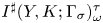 $I^{\sharp }(Y, K; \Gamma _{\sigma })^{\tau }_{\omega }$ as being independent of the choice of framing
 $\tau$. Note, however, that if
 $\tau _{0}$ and
 $\tau _{1}$ are framings which are equal mod
 $2$, then the corresponding local systems are identical, but our chosen canonical isomorphism is not the identity map: it is multiplication by
 $T_{0}^{n}$, where
 $n$ is half the difference between the framings.
Henceforth, we will continue to omit  $\tau$ from our notation. When the ambient cobordism
 $X$ is a cylinder, or is otherwise understood, we will simply write
 \begin{equation} I^{\sharp}(S ; \Gamma_{\sigma})_{\omega} : I^{\sharp}( K_{0}; \Gamma_{\sigma})_{\omega_{0}} \to I^{\sharp}( K_{1}; \Gamma_{\sigma})_{\omega} \end{equation}
for the map (20).
2.5 A reduced variant
The instanton homology  $I^{\sharp }(K)$ with constant coefficients has a ‘reduced’ version
 $I^{\natural }(K)$, which is described, for example, in [Reference Kronheimer and MrowkaKM12]. It depends on a choice of base point on the link
 $K$, and the relationship of
 $I^{\natural }$ to
 $I^{\sharp }$ is similar to the relationship between the reduced and unreduced versions of Khovanov homology [Reference KhovanovKho00]. Given a base change
 $\sigma : \mathcal {R}\to \mathcal {S}$ satisfying the extra condition
 $\sigma (T_{0})=\sigma (T_{1})$, we can construct a reduced version
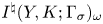 $I^{\natural }(Y,K;\Gamma _{\sigma })_{\omega }$ of
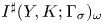 $I^{\sharp }(Y,K;\Gamma _{\sigma })_{\omega }$, for knots and links
 $K\subset Y$. We describe the construction here.
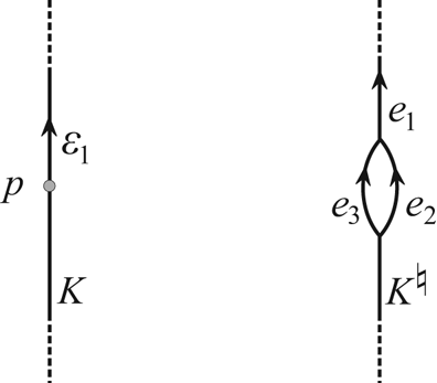
Let  $K\subset Y$ be a link. Let
 $p$ be the base point on
 $K$ and
 $(\epsilon _{1}, \epsilon _{2}, \epsilon _{3})$ be an oriented basis of tangent vectors with
 $\epsilon _{1}$ pointing along
 $K$. Making the modification in a standard ball around
 $p$, create a spatial graph with two vertices by replacing an arc of
 $K$ adjacent to
 $p$ with a bigon, as shown in Figure 1. Let
 $K^{\natural }\subset Y$ denote the resulting web. Let
 $\mathcal {B}^{\natural }(Y, K)$, or just
 $\mathcal {B}^{\natural }(K)$, denote the space of marked bifold connections on the corresponding bifold.
A knot  $K$ with base point
 $p$ and the resulting web
 $K^{\natural }$ obtained by adding a bigon.

We define three circle-valued functions,
 \[ \big(h_{1}, h_{2}, h_{3}\big) : \mathcal{B}^{\natural}(K) \to \mathbb{R}^{3}/\mathbb{Z}^{3}, \]
as follows. First, in the case that  $K$ is a knot, the web
 $K^{\natural }$ is the union of three oriented arcs
 $e_{1}$,
 $e_{2}$,
 $e_{3}$, where
 $e_{2}$ and
 $e_{3}$ comprise the added bigon. All three are oriented by
 $\epsilon _{1}$. As before, the structure group of a connection
 $[A]\in \mathcal {B}^{\natural }(K)$ reduces to
 $S^{1}$ along the arcs, and the holonomy of
 $[A]$ along the three arcs defines the maps
 $h_{i}$, just as in the case of
 $\mathcal {B}^{\sharp }(K)$. If
 $K$ is a link, let
 \[ h_{0} : \mathcal{B}^{\natural}(K) \to \mathbb{R}/\mathbb{Z} \]
be obtained from the holonomy along the remaining components of  $K$ (those that do not contain
 $p$). In the case of a knot, just take
 $h_{0}$ to be constant. In either case, we now have a map
 \[ \big(h_{0},h_{1}, h_{2}, h_{3}\big) \to \mathbb{R}^{4}/\mathbb{Z}^{4}, \]
from which we can construct a local system of  $\mathcal {R}$-modules
 $\Gamma$ over
 $\mathcal {B}^{\natural }(K)$ as before. In the case that the base change
 $\sigma : \mathcal {R}\to \mathcal {S}$ has
 $\sigma (T_{0}) = \sigma (T_{1})$, the local system is pulled back from
 $\mathbb{R}^{3}/ \mathbb{Z}^{3}$ via the map
 \[ \mathbb{R}^{4}/\mathbb{Z}^{4} \to \mathbb{R}^{3}/\mathbb{Z}^{3}, \]
which adds the first two components. We shall consider only cases such as this when discussing reduced instanton homology in this paper, in order to have the components of  $K$ on an equal footing. We then define
 $I^{\natural }(K; \Gamma _{\sigma })$ using the Morse homology of the perturbed Chern–Simons functional on
 $\mathcal {B}^{\natural }(K)$, with coefficients in
 $\Gamma _{\sigma }$.
This reduced instanton homology is functorial for ‘based’ cobordisms of links. Given links  $(Y_{0}, K_{0})$ and
 $(Y_{1}, K_{1})$, with framed base points
 $p_{0}$ and
 $p_{1}$ on the links, the appropriate morphism is given by a cobordism of pairs,
 $(X,S)$, together with an arc
 $\gamma \subset S$ joining the base points and a framing
 $(\epsilon _{1}, \epsilon _{2}, \epsilon _{3})$ of the normal to
 $\gamma$ in
 $X$ such that
 $\epsilon _{1}$ is tangent to
 $S$. Equivalently, we can think of an embedding of
 $[0,1]\times B^{3}$ in
 $X$ which intersects
 $S$ in the image of the standard
 $[0,1]\times B^{1}$. Given such data, we can perform the bigon addition (Figure 1) in a one-parameter family along the image of
 $[0,1]\times B^{3}$, to obtain an embedded foam
 $S^{\natural }$ with boundary
 $K^{\natural }_{0} \cup K^{\natural }_{1}$. The foam gives rise to homomorphisms
 \[ I^{\natural}\big(X,S; \Gamma_{\sigma}\big) : I^{\natural}\big(Y_{0}, K_{0}; \Gamma_{\sigma}\big) \to I^{\natural}\big(Y_{1}, K_{1}; \Gamma_{\sigma}\big), \]
where the matrix entries at the chain level are given by the same formulae (22) as in the non-reduced case, with the  $\nu _{i}$ being the curvature integrals over the facets of
 $S^{\natural }$.
The naming of  $I^{\natural }(Y, K; \Gamma _{\sigma })$ as the reduced variant is justified by its relationship to (for example) the reduced version of Bar-Natan homology, as described in Corollary 6.6. We shall see later that, while
 $I^{\sharp }(U ; \Gamma _{\sigma })$ for the unknot
 $U$ is a free module of rank 2, the reduced version has rank
 $1$. As in [Reference Kronheimer and MrowkaKM12], there is an exact triangle relating the reduced homology (twice) to the unreduced homology.
2.6 The Künneth theorem for reduced homology
Given links  $K_{1}$ and
 $K_{2}$, each with a framed base point, there is a natural construction of the connected sum
 $K_{1}\mathbin {\#} K_{2}$, also as a link with a framed base point. To spell this out, let
 $(\epsilon _{1}, \epsilon _{2}, \epsilon _{3})$ be the framing at the base point of
 $K_{1}$, with
 $\epsilon _{1}$ pointing along the knot. Using the framing, parametrize a standard ball
 $B_{3,1}$ around the base point. Construct
 $B_{3,2}$ similarly. Remove the interiors and form the connected sum by identifying the
 $2$-sphere
 $\partial B_{3,1}$ with
 $\partial B_{3,2}$ using the orientation-reversing diffeomorphism given by reflection in the
 $\epsilon _{1}$ direction. Take the base point on the new link to be the image of the point
 $\epsilon _{1}$ on
 $\partial B_{3,1}$.
The construction of  $K_{1}\mathbin {\#} K_{2}$ from the two framed knots is functorial. That is, given cobordisms
 $S_{i}$ from
 $K_{i}'$ to
 $K_{i}$ for
 $i=1,2$, and given framed arcs
 $\gamma =(\gamma _{1}, \gamma _{2})$ joining the framed base points, we can form a cobordism
 \[ S_{1} \mathbin{\#}_{\gamma} S_{2} \]
from  $K'_{1}\mathbin {\#} K_{2}'$ to
 $K_{1}\mathbin {\#} K_{2}$ by performing the connected-sum construction in an interval family. The reduced instanton homology for a connected sum of framed knots is described as a tensor product by a Künneth theorem.
Proposition 2.4 Let  $(C_{1}, \partial )$ and
 $(C_{2},\partial )$ be the differential
 $\mathcal {S}$-modules arising from the Floer complexes for the homology groups
 $I^{\natural }(K_{1};\Gamma _{\sigma })$ and
 $I^{\natural }(K_{2};\Gamma _{\sigma })$. Then the Floer complex for
 $K_{1}\mathbin {\#} K_{2}$ is chain-homotopy equivalent to the tensor product
 $C_{1}\otimes _{\mathcal {S}} C_{2}$. In particular, if
 $\mathcal {S}$ is a principal ideal domain, then there is a split exact sequence of
 $\mathcal {S}$-modules,
 \begin{align} &0 \longrightarrow I^{\natural}(K_{1};\Gamma_{\sigma}) \otimes_{\mathcal{S}} I^{\natural}(K_{2};\Gamma_{\sigma}) \longrightarrow I^{\natural}(K_{1}\mathbin{\#} K_{2};\Gamma_{\sigma})\nonumber\\ &\,\,\,\longrightarrow \mathrm{Tor}^{\mathcal{S}}_{1} (I^{\natural} (K_{1};\Gamma_{\sigma} ), I^{\natural}(K_{2};\Gamma_{\sigma}) ) \longrightarrow 0. \end{align}
The exact sequence, but not the splitting, is natural with respect to the maps induced by cobordisms  $S_{1}$,
 $S_{2}$ and
 $S_{1}\mathbin {\#}_{\gamma }S_{2}$ as constructed above.
Proof. This a standard application of excision, as we now describe. The symmetries in the argument are more apparent in a more general version, so we consider four pairs  $(Y_{i}, K_{i})$,
 $k=1,\ldots ,4$, where each
 $K_{i}$ is a based link. For each
 $i\ne j$, there is a connect sum of pairs,
 \[ (Y_{ij},K_{ij}) = (Y_{i} , K_{i}) \mathbin{\#} (Y_{j}, K_{j}), \]
where the 3-manifolds and the links are both summed at the base points. Let  $C^{\natural }_{ij}$ denote the chain group of free
 $\mathcal {S}$-modules arising as the instanton Floer complex for this connected sum of based pairs, with coefficients in the local system
 $\Gamma _{\sigma }$. The more general statement is then that there is a chain-homotopy equivalence,
 \begin{equation} C^{\natural}_{12} \otimes_{\mathcal{S}} C^{\natural}_{34} \simeq C^{\natural}_{13} \otimes_{\mathcal{S}} C^{\natural}_{24}, \end{equation}
and that the resulting maps on homology are natural for cobordisms. The statement of the original proposition arises as a special case, when each  $Y_{i}$ is
 $S^{3}$, and
 $K_{3}$ and
 $K_{4}$ are both the unknot, so that
 $(Y_{13}, K_{13})=(Y_{1}, K_{1})$,
 $(Y_{24}, K_{24})=(Y_{2}, K_{2})$ and
 $C^{\natural }_{34}=\mathcal {S}$.
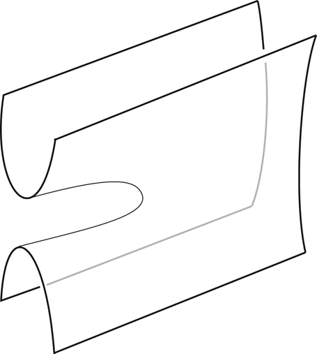
We now recall Floer's excision argument, particularly in the versions described in [Reference Kronheimer and MrowkaKM19b, Proposition 4.2] and [Reference Kronheimer and MrowkaKM19a, Proposition 3.3]. Let  $U$ be as in Figure 2, a two-dimensional cobordism from the one-dimensional manifold-with-boundary
 $I\cup I$ to
 $I\cup I$. Take the product with
 $S^{2}$ to obtain a cobordism from
 $I\times S^{2}\cup I\times S^{2}$ to
 $I\times S^{2} \cup I\times S^{2}$. Then attach four copies of
 $[0,1]\times B^{3}$ to obtain a cobordism
 $W$ from
 $S^{3}\cup S^{3}$ to
 $S^{3}\cup S^{3}$. Inside
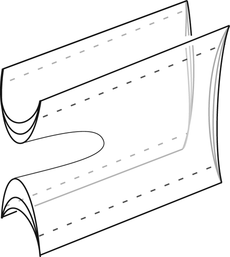
 $W$ there is an embedded foam,
 $\Phi$, formed from three copies of
 $U$. The pair
 $(W,\Phi )$ is a cobordism
 \[ (S^{3},\theta) \cup (S^{3},\theta)\quad \text{to}\quad (S^{3},\theta) \cup (S^{3},\theta). \]
On one facet of the three facets of  $\Phi$, let
 $\gamma _{i}$,
 $i=1,\ldots ,4$, be four arcs as shown in Figure 3. A regular neighborhood of
 $\gamma _{i}$ in
 $(W,\Phi )$ is a standard pair
 $[0,1]\times (B^{3}, B^{1})$ along which we form a sum with
 $[0,1]\times (Y_{i}, K_{i})$. The result is a cobordism of pairs,
 $(X,\Psi )$, from
 \[ \big(Y_{12}, K_{12}^{\natural}\big) \cup \big(Y_{34}, K_{34}^{\natural}\big) \quad \text{to}\quad \big(Y_{13}, K_{13}^{\natural}\big) \cup \big(Y_{24}, K_{24}^{\natural}\big). \]
As in the proof of [Reference Kronheimer and MrowkaKM19a, Proposition 3.3], this cobordism of pairs gives rise to a map on the instanton chain complexes with local coefficients, in this case a chain map
 \[ C^{\natural}_{12} \otimes_{\mathcal{S}} C^{\natural}_{34} \to C^{\natural}_{13} \otimes_{\mathcal{S}} C^{\natural}_{24}. \]
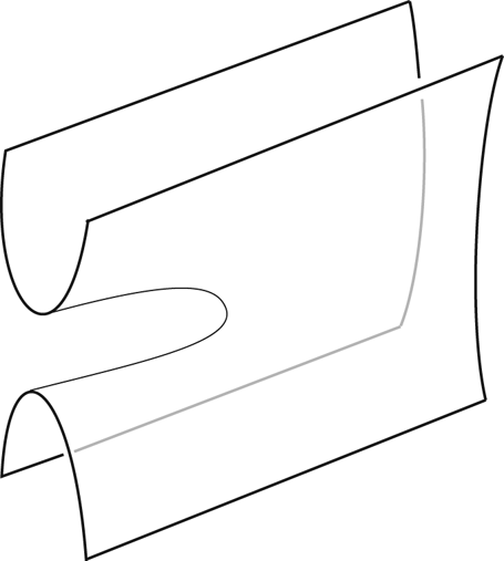
The cobordism  $U$ from two copies of an interval
 $I$ to another two.
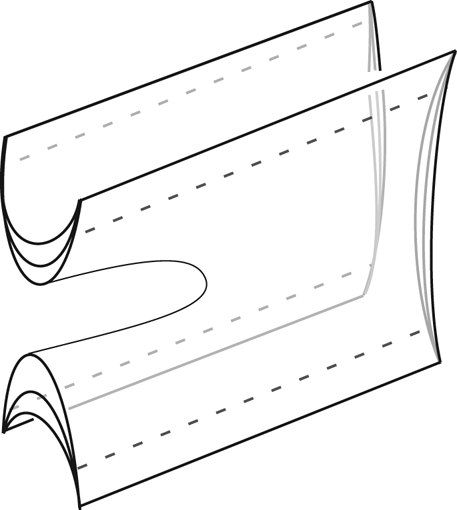
The foam  $\Phi \subset W$ and the four arcs along which the pairs
 $[0,1]\times (Y_{i},K_{i})$ are summed.
By the same construction, a map in the other direction is constructed. The fact that the composite of the two, in either order, is chain-homotopic to the identity is proved by the usual argument, as in [Reference Kronheimer and MrowkaKM19a] for example.
3. Operators on $I^{\sharp }(K;\Gamma )$

We continue with the notation of the previous sections. We write  $Y^{o}\subset Y$ for the complement of a ball around a base point in
 $Y$, and we consider a link
 $K\subset Y^{o}$, along with the union
 $K^{\sharp } = K\cup \theta$ in
 $Y$. The space of connections
 $\mathcal {B}^{\sharp }(K)_{\omega }$ carries a system of local coefficients
 $\Gamma _{\sigma }$, as in Notation 2.3), and
 $I^{\sharp }(K ; \Gamma _{\sigma })_{\omega }$ is the instanton homology for the perturbed Chern–Simons functional on
 $\mathcal {B}^{\sharp }(K)_{\omega }$, with coefficients in the local system.
3.1 Operators from characteristic classes of the base-point bundle
Given a point  $y$ in the smooth part of the orbifold
 $(Y, K)$, there is a base-point
 $\mathop {{SO}}(3)$-bundle
 $\mathbb{E}_{y}$ on the configuration space, with Stiefel–Whitney classes
 \[ \mathsf{w}_{1} , \mathsf{w}_{2}, \mathsf{w}_{3} \in H^{*}\big(\mathcal{B}^{\sharp}(K)_{\omega}; \mathbb{Z}/2\big). \]
(See [Reference Kronheimer and MrowkaKM19a, § 4].) For the instanton homology  $I^{\sharp }(K ;\Gamma _{\sigma })$, these characteristic classes give rise to linear operators,
 \[ w_{i} : I^{\sharp}(K ; \Gamma_{\sigma})_{\omega} \to I^{\sharp}(K ; \Gamma_{\sigma})_{\omega}. \]
The definition of these for the similar case of  $J^{\sharp }(K ; \Gamma _{\theta })$ is presented in [Reference Kronheimer and MrowkaKM19a] and needs essentially no change. As in [Reference Kronheimer and MrowkaKM19a], we have the following result.
Lemma 3.1 On  $I^{\sharp }(K;\Gamma _{\sigma })_{\omega }$, the operators
 $w_{1}$ and
 $w_{3}$ are zero, while
 $w_{2}$ is multiplication by
 $\sigma (P)\in \mathcal {S}$, where
 $P\in \mathcal {R}$ is the element given by the expression in (5).
3.2 A two-dimensional cohomology class
Let  $a$ be an arc in
 $Y$ with end points
 $\{p,q\}$ on
 $K\cup \theta$. The interesting case will be when
 $p$ and
 $q$ lie on different components, for example on
 $K$ and
 $\theta$, respectively. We require that
 $p$ and
 $q$ lie on the interior of edges, not at the vertices of the graph. We also require that
 $p$ and
 $q$ do not lie at end points of
 $\omega$ (if any). There is a universal
 $\mathbb{R}^{3}$ bundle
 \[ \mathbb{E} \to a \times \mathcal{B}^{\sharp}(K)_{\omega}. \]
The restriction,  $\mathbb{E}_{p}$, of
 $\mathbb{E}$ to the end point
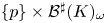 $\{p\} \times \mathcal {B}^{\sharp }(K)_{\omega }$ carries an involution on the
 $\mathbb{R}^{3}$ fibers, because of the
 $\mathbb{Z}/2$ stabilizer at this singular point of the orbifold, so
 $\mathbb{E}_{p}$ contains a distinguished real line subbundle, the
 $+1$ eigenspace of the involution:
 \[ \mathbb{L}_{p} \subset \mathbb{E}_{p} \to \mathcal{B}^{\sharp}(K)_{\omega}. \]
This line bundle is trivial. Indeed, we have the following result.
Lemma 3.2 Given the condition that  $p$ is not a boundary point of
 $\omega$, a choice of orientation
 $o_{p}$ for
 $\mathbb{L}_{p}$ is determined by an orientation of
 $K$ at
 $p$. If
 $p_{1}$ and
 $p_{2}$ lie either side of a single end point of
 $\omega$ on
 $K$, and if
 $K$ is given the same orientation at
 $p_{1}$ and
 $p_{2}$, then the corresponding orientations
 $o_{p_{1}}$,
 $o_{p_{2}}$ of
 $\mathbb{L}_{p_{1}} \cong \mathbb{L}_{p_{2}}$ are opposite.
Proof. We use the characterization of  $\mathcal {B}^{\sharp }(K)_{\omega }$ in Lemma 2.2. The connection
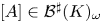 $[A]\in \mathcal {B}^{\sharp }(K)_{\omega }$ has a preferred lift to an
 $\mathop {{SU}}\nolimits (2)$ connection
 $\hat {A}$ in
 $U_{p}{\setminus} K$ for some neighborhood
 $U_{p}$ of
 $p$ in
 $Y$. After orienting (the normal bundle to)
 $K$, we can consider the limiting holonomy of
 $\hat {A}$ around small circles linking
 $p\in K$, which is an element of order
 $4$ in
 $\mathop {{SU}}\nolimits (2)$. The 2-sphere which parametrizes elements of order
 $4$ is identified with the unit sphere in the
 $\mathbb{R}^{3}$ bundle, and under this identification the limiting holonomy is an element of
 $\mathbb{L}_{p}$.
With the lemma in mind, we introduce the following notation.
Definition 3.3 A dot on  $K$ is a chosen point
 $p$ on
 $K$, not a boundary point of
 $\omega$, together with a choice of orientation
 $o_{p}$ for the line bundle
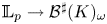 $\mathbb{L}_{p}\to \mathcal {B}^{\sharp }(K)_{\omega }$. We may omit explicit mention of
 $o_{p}$ and simply refer to
 $p$ as a dot. If
 $p$ is a dot, we write
 $\bar {p}$ for a dot with the same underlying point and the opposite orientation for the line bundle. We note that a choice of orientation of
 $\mathbb{L}_{p}$ is equivalent to a choice of orientation of
 $K$ near
 $p$.
Suppose now that  $p$ and
 $q$ are dots; let us return to the arc
 $a$ joining them as introduced above. The dot
 $p$ determines a distinguished section of
 $\mathbb{L}_{p}$ and hence a distinguished section
 $i_{p}$ of the
 $\mathbb{R}^{3}$ bundle
 $\mathbb{E}_{p}$. Similarly, using the dot
 $q$, we obtain a distinguished section
 $i_{q}$. Changing the sign of the second one, we obtain a distinguished section
 \[ I = (i_{p} , -i_{q}) \]
of the restriction of  $\mathbb{E}$ to
 $\partial a \times \mathcal {B}^{\sharp }(K)$.
The distinguished section on the boundary allows us to define a relative Euler class or a top Stiefel–Whitney class
 \begin{align*} {\mathbb w}_{3} &= w_{3}(\mathbb{E} , I) \\ & \in H^{3} ((a, \partial a ) \times \mathcal{B}^{\sharp}(K) ; \mathbb{F}_{2} ). \end{align*}
We now take the slant product with the relative fundamental class of the arc to obtain a class on  $\mathcal {B}^{\sharp }(K)_{\omega }$.
Definition 3.4 For an arc  $a$ as above whose end points
 $p$ and
 $q$ are dots, we define a two-dimensional cohomology class with
 $\mathbb{F}_{2}$ coefficients on
 $\mathcal {B}^{\sharp }(K)_{\omega }$ as
 \begin{align} \lambda &= {\mathbb w}_{3} / [a, \partial a] \nonumber\\ &\in H^{2} ( \mathcal{B}^{\sharp}(K) ; \mathbb{F}_{2} ). \end{align}
The next lemma shows that the arc  $a$ itself plays only an auxiliary role in this construction.
Lemma 3.5 In the above construction, the class  $\lambda$ depends only on the dots
 $p$,
 $q$. It does not otherwise depend on the arc
 $a$.
Proof. Consider the universal  $\mathbb{R}^{3}$ bundle
 \[ \mathbb{E} \to (Y{\setminus} K) \times \mathcal{B}^{\sharp}(K)_{\omega}. \]
The assertion to be proved is equivalent to the statement that
 \begin{align*} w_{3}(\mathbb{E}) / [b] & = 0 \\ &\in H^{2} ( \mathcal{B}^{\sharp}(K)_{\omega} ; \mathbb{F}_{2} ) \end{align*}
for any 1-cycle  $b$ in
 $Y{\setminus} K$. The bundle has trivial
 $w_{2}$ on
 $Y{\setminus} K$, so each irreducible connection lifts to an
 $\mathop {{SU}}\nolimits (2)$ connection with stabilizer
 $\pm 1$. This means that
 $w_{2}(\mathbb{E})$ can be represented by a
 $2$-cocycle which is pulled back from
 $\mathcal {B}^{\sharp }(K)_{\omega }$. The class
 $w_{3}$ is obtained by applying a Bockstein homomorphism to
 $w_{2}$. So, the class
 $w_{3}(\mathbb{E})$ is also pulled back from
 $\mathcal {B}^{\sharp }(K)_{\omega }$. It follows that
 $w_{3}(\mathbb{E}) / [b]$ is zero for all
 $1$-cycles
 $b$ in
 $Y{\setminus} K$ (and incidentally all
 $2$-cycles also).
The lemma allows us to write the class as a function of the two dots,
 \begin{equation} \lambda_{pq} \in H^{2}\big(\mathcal{B}^{\sharp}(K) ; \mathbb{F}_{2} \big). \end{equation}
The next lemma asks how  $\lambda _{pq}$ changes if we change the orientation
 $o_{q}$ at one end point: that is, we replace
 $q$ by
 $\bar {q}$. We introduce the following notation: we write
 \[ \lambda'_{pq} = \lambda_{p\bar{q}}. \]
Lemma 3.6 Let  $p$ and
 $q$ be dots, and let
 $\lambda _{pq}$ and
 $\lambda '_{pq}$ be the resulting classes, as above. Then these classes satisfy the relations
 \begin{equation} \begin{aligned} \lambda_{pq} + \lambda'_{pq} & = w_{2}(\mathbb{E}_{q}), \\ \lambda_{pq} \lambda'_{pq} & = 0. \end{aligned} \end{equation}
Proof. Because of the independence of the choice of arc, and the way the signs are used in the definition of  $I$ above, the first relation is equivalent to saying that
 \[ \lambda_{qq} = w_{2}(\mathbb{E}_{q}), \]
where the left-hand side can be computed using the constant arc from  $q$ to
 $q$.
The general statement at the level of characteristic classes is the following. Suppose that we have an  $\mathbb{R}^{3}$ bundle
 $E\to T$ with a section
 $i_{0}$. Consider the pull-back
 $\pi ^{*}(E)$ to
 $[0,1]\times T$ with a section
 $I$ which is equal to
 $i_{0}$ on
 $\{0\}\times T$ and
 $-i_{0}$ on
 $\{1\}\times T$. Then the result of slanting
 $w_{3}(\pi ^{*}(E), I)$ with the fundamental class of
 $[0,1]$ is
 $w_{2}(E)$:
 \[ w_{3}(\pi^{*}(E), I)/ [0,1] = w_{2}(E). \]
This can be verified by pulling back  $E$ to
 $S^{1}\times T$ and tensoring by the Möbius bundle
 $\mu$ on
 $S^{1}$, in which case the assertion is
 \[ w_{3}(\pi^{*}(E)\otimes \mu )/ [S^{1}] = w_{2}(E). \]
In this form, the verification is straightforward, using the splitting principle. This completes the proof of the first relation.
To set the second relation in a more general context, consider again an  $\mathbb{R}^{3}$ bundle
 $E\to T$ with two non-vanishing sections
 $i_{0}$ and
 $i_{1}$. Let
 $I$ be a path of sections, from
 $i_{0}$ to
 $-i_{1}$, through sections which may vanish: we take explicitly
 \[ I(t) = (1-t) i_{0} - t i_{1}. \]
Similarly, let  $I'(s)$ be the path from
 $i_{0}$ to
 $i_{1}$ given by
 \[ I'(s) = (1-s) i_{0} + s i_{1}. \]
We have cohomology classes by
 \begin{align*} \lambda&=w_{3}(E,I)/[0,1]\\ & \in H^{2}(T;\mathbb{F}_{2}), \\ \lambda'&= w_{3}(E, I')/[0,1]\\ & \in H^{2}(T;\mathbb{F}_{2}), \end{align*}
where we now interpret  $I$ and
 $I'$ as sections on
 $[0,1]\times T$ that are non-zero at the boundaries. To show that
 $\lambda \lambda '=0$, it is sufficient to show that there is no
 $(t,s)$ in the interior of
 $[0,1]\times [0,1]$ for which the sections
 $I(t)$ and
 $I'(s)$ have a common zero in
 $T$. A necessary condition for a common zero is that the determinant of the matrix
 \[ \begin{pmatrix} (1-t) & -t \\ (1-s) & s \end{pmatrix} \]
is zero. But the determinant is  $s+t-2st$, which is strictly positive on the interior of
 $[0,1]\times [0,1]$. The result follows.
Corollary 3.7 The class  $\lambda _{pq}$ satisfies the relation
 \[ \lambda^{2}_{pq} + w_{2}(\mathbb{E}_{q}) \lambda_{pq} = 0. \]
Proof. This is an immediate corollary of the two relations in the lemma.
3.3 Operators from the two-dimensional classes
In the usual way, and following the exposition in [Reference Kronheimer and MrowkaKM19a], the cohomology class  $\lambda _{pq}$ gives rise to an operator
 \begin{equation} \Lambda_{pq} : I^{\sharp}(Y, K ; \Gamma_{\sigma})_{\omega} \to I^{\sharp}(Y, K ; \Gamma_{\sigma})_{\omega}. \end{equation}
In a little more detail, let  $a$ be the chosen arc joining the two dots, regarded as subset of the cylinder
 $\check X = \mathbb{R}\times \check Y$, in the slice where the
 $\mathbb{R}$ coordinate is zero. Following [Reference Kronheimer and MrowkaKM19a, § 4.3], let
 $Z\subset \check X$ be a subset of
 $\check X$ which includes a neighborhood of
 $a$ and such that the restriction map
 \[ H^{1}(Y{\setminus} K; \mathbb{F}_{2}) \to H^{1}(Z{\setminus} K; \mathbb{F}_{2}) \]
is injective. The latter condition means that there is a well-defined restriction map for marked connections,
 \[ M(\alpha, \beta) \to \mathcal{B}^{*}(Z ; \mu_{Z}), \]
where  $\mu _{Z}$ is the intersection with
 $Z$ of the marking data
 $\mathbb{R}\times \mu _{\omega }$. Because
 $Z$ contains a neighborhood of
 $a$, the class
 $\lambda _{pq}$ can be defined on
 $\mathcal {B}^{*}(Z ; \mu _{Z})$, where it is dual to a stratified codimension-2 subvariety
 $V$. The matrix entries of
 $\Lambda _{pq}$ at the chain level are defined by counting points of the intersections
 \[ M(\alpha, \beta) \cap V \]
and weighting them using the local system. As in [Reference Kronheimer and MrowkaKM19a], the necessary compactness results hold because the cohomology class has dimension  $2$ and
 $Z$ can be chosen so that it meets the foam only in the faces (at neighborhoods of
 $p$ and
 $q$).
Using notation that is parallel to the notation for  $\lambda _{pq}$ and
 $\lambda '_{pq}$, we write
 $\Lambda '_{pq}$ for the operator of the same form as (29), but using
 $\bar {q}$ in place of
 $q$. The relations in Lemma 3.6, satisfied by
 $\lambda _{pq}$ and
 $\lambda '_{pq}$, give rise to relations satisfied by the corresponding operators on Floer homology.
Lemma 3.8 Let  $\Lambda _{pq}$ and
 $\Lambda '_{pq}$ be the operators on
 $I^{\sharp }(K;\Gamma _{\sigma })_{\omega }$ arising from a pair of dots
 $\{p,q\}$ as above. Then these operators satisfy the relations
 \begin{equation} \begin{aligned} \Lambda_{pq} + \Lambda'_{pq} & = \sigma(P), \\ \Lambda_{pq} \Lambda'_{pq} & = \sigma(Q_{pq}), \end{aligned} \end{equation}
where  $P$ is the element of
 $\mathcal {R}$ given by (5), and
 \[ Q_{pq} = \big(T_{m_{p}}^{2} + T_{m_{p}}^{{-}2}\big) + \big(T_{m_{q}}^{2} + T_{m_{q}}^{{-}2}\big). \]
In the above formula,  $T_{m_{p}}$ and
 $T_{m_{q}}$ are the variables from
 $\{T_{0}, T_{1}, T_{2}, T_{3}\}$ associated to the edges of
 $K \cup \theta$ on which
 $p$ and
 $q$ lie. Thus,
 $m_{p}=1, 2$ or
 $3$ if
 $p$ lies on the edge
 $e_{1}$,
 $e_2$ or
 $e_{3}$ of
 $\theta$, and
 $m_{p}=0$ if
 $p$ lies on
 $K$.
Proof. By an excision argument [Reference Kronheimer and MrowkaKM12], it is sufficient to prove this in the case that  $\omega$ is empty. It is then sufficient to consider the case that the base change
 $\sigma$ is the identity.
The first of the two relations follows from the corresponding formula for  $\lambda _{pq} + \lambda '_{pq}$ in Lemma 3.6, together with the formula
 $w_{2}=P$ from Lemma 3.1.
The second relation, for the product, is more subtle, because it involves a four-dimensional moduli space, and there is a contribution from codimension-4 bubbling which may occur at the end points  $p$ and
 $q$ of the arc
 $a \subset Z$.
As in [Reference XieXie16] and [Reference Kronheimer and MrowkaKM19a], the contributions from the bubbles at  $p$ and
 $q$ are universal quantities, so that the relation for the product has the general shape
 \[ \Lambda_{pq} \Lambda'_{pq} = F(T_{m_{p}}) + F(T_{m_{q}}), \]
where  $F$ is universal and is a finite Laurent series in one variable. To compute
 $F$, we take as a special case the situation that
 $K$ is empty and
 $p$ and
 $q$ lie on the edges
 $e_{2}$ and
 $e_{1}$ of
 $\theta$, respectively. In the ring
 $\mathbb{F}_{2}[T_{1}^{\pm 1}, T_{2}^{\pm 1}, T_{3}^{\pm 1}]$, we then have elements
 $\Lambda$ and
 $\Lambda '$ with relations
 \begin{align*} \Lambda + \Lambda' &= P \\ &= T_{1}T_{2}T_{3} + T_{1}T_{2}^{{-}1}T_{3}^{{-}1} + T_{2}T_{3}^{{-}1}T_{1}^{{-}1} + T_{3}T_{1}^{{-}1}T_{2}^{{-}1} \end{align*}
and
 \[ \Lambda \Lambda' = F(T_{2}) + F(T_{1}). \]
The only way to solve the constraint that  $\Lambda \Lambda '$ is a function of
 $T_{1}$ and
 $T_{2}$ only is to have the general shape
 \begin{align*} \Lambda & = T_{3}^{a} G(T_{1}, T_{2}), \\ \Lambda'& = T_{3}^{{-}a} H(T_{1}, T_{2}) \end{align*}
for some Laurent polynomials  $G$ and
 $H$ in two variables. The shape of the formula for
 $\Lambda +\Lambda '$ tells us that
 $a$ must be
 $\pm 1$ and that
 $\Lambda$ and
 $\Lambda '$ must consist of the corresponding monomials from the formula for
 $P$. Thus,
 \begin{equation} \begin{aligned} \Lambda & = T_{3}\big(T_{1}T_{2} + T_{1}^{{-}1}T_{2}^{{-}1}\big), \\ \Lambda' & = T_{3}^{{-}1}\big(T_{1}^{{-}1}T_{2} + T_{1}T_{2}^{{-}1}\big) \end{aligned} \end{equation}
or vice versa. Either way, we have  $F(T)= T^{2} + T^{-2}$.
As with the cohomology classes themselves, we have an immediate corollary of the lemma, for the operator  $\Lambda _{pq}$.
Corollary 3.9 The operator  $\Lambda _{pq}$ satisfies the relation
 \[ \Lambda^{2}_{pq} +\sigma( P) \Lambda_{pq} + \sigma(Q_{pq}) = 0. \]
To create an operator that treats the three edges of  $\theta$ symmetrically, we make the following definition.
Definition 3.10 Fix once and for all a dot  $p_{m}$ on each edge
 $e_{m}$ of
 $\theta$ for
 $m=1,2,3$. Then, given a dot
 $q$ on the link
 $K$, we define
 \[ \Lambda_{q} = \Lambda_{p_{1}q} + \Lambda_{p_{2}q} + \Lambda_{p_{3}q}, \]
with  $\Lambda '_{q}$ defined similarly.
Corollary 3.11 The operator  $\Lambda _{q}$ above satisfies the relation
 \[ \Lambda^{2}_{q} + \sigma(P) \Lambda_{q} +\sigma( Q) = 0, \]
where  $P$ and
 $Q$ are given by the formulae in (5). Furthermore,
 $\Lambda _{q} + \Lambda '_{q}= \sigma (P)$.
Proof. We are in characteristic  $2$, where squaring is linear. The
 $Q$ that appears in the quadratic relations is now the sum of the terms
 $Q_{p_{m} q}$ for
 $m=1,2,3$.
3.4 Surfaces with dots
The operators  $\Lambda _{q}$ on
 $I^{\sharp }(K;\Gamma _{\sigma })_{\omega }$ that we have defined can be combined, in the usual way, with the functorial maps obtained from cobordisms
 $S$ between knots and links. Thus, suppose that we are given a cobordism
 $(X,S)$ from
 $(Y_{0},K_{0})$ to
 $(Y_{1}, K_{1})$ as in (23), and let
 $q$ be a dot on
 $S$. As before, this means a point with a choice of orientation
 $o_{q}$ of the line bundle
 $\mathbb{L}_{q}$. We then obtain a map
 \begin{equation} I^{\sharp}((S;q) ; \Gamma_{\sigma})_{\omega} : I^{\sharp}( K_{0}; \Gamma_{\sigma})_{\omega_{0}} \to I^{\sharp}( K_{1}; \Gamma_{\sigma})_{\omega_{1}}. \end{equation}
If  $q$ can be joined by a path on
 $S$ to a point
 $q_{0}\in K_{0}$ (respectively, a point
 $q_{1}\in K_{1}$), then this map is equal to the composite,
 \[ I^{\sharp}(S ; \Gamma_{\sigma})_{\omega} \circ \Lambda_{q_{0}}, \]
respectively,
 \[ \Lambda_{q_{1}} \circ I^{\sharp}(S ; \Gamma_{\sigma})_{\omega}. \]
The functorial properties of  $I^{\sharp }$ extend to this larger category in which the morphisms are ‘cobordisms with dots’. We note that, as with the case of dots on a link
 $K$, an orientation of the line bundle
 $\mathbb{L}_{q}$ is equivalent to a choice of orientation for a neighborhood of
 $q$ in
 $S$. So, a dot can be regarded as point in
 $S$ together with an orientation of
 $T_{q}S$.
4. Double points and handles
As in § 2.4, let  $Y_{0}$,
 $Y_{1}$ be 3-manifolds with base points, containing links
 $K_{0}$,
 $K_{1}$, and let
 $\omega _{0}$,
 $\omega _{1}$ be representatives for the Stiefel–Whitney class. We continue to use
 $\Gamma _{\sigma }$ to denote
 $\Gamma \otimes _{\sigma } \mathcal {S}$, and we consider again a map
 \begin{equation} I^{\sharp}(X, S; \Gamma_{\sigma})_{\omega} : I^{\sharp}(K_{0}; \Gamma_{\sigma})_{\omega_{0}} \to I^{\sharp}(K_{1} ; \Gamma_{\sigma})_{\omega_{1}} \end{equation}
arising from a bifold cobordism  $(X,S)$ and a choice of Stiefel–Whitney class represented by a surface
 $\omega$ with boundary. We continue to assume that
 $S$ is a surface rather than a more general foam, and we recall that
 $\omega$ is allowed to have part of its boundary on
 $S$ if
 $\sigma (T_{0})=1$. Implicit in our notation is an embedding of
 $[0,1]\times B^{3}$ in
 $X$, containing the cylindrical foam
 $[0,1]\times \theta$, disjoint from
 $S$ and
 $\omega$.
As in [Reference Kronheimer and MrowkaKM12, Reference Kronheimer and MrowkaKM19b, Reference Kronheimer and MrowkaKM19a], we can consider how the map 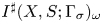 $I^{\sharp }(X,S ; \Gamma _{\sigma })_{\omega }$ changes when we modify the topology of
 $S$ in standard ways.
4.1 Connect sum with $\mathbb{R}\mathbb{P}^{2}$

In  $S^{4}$, there are two standard copies of
 $\mathop {\mathbb{R}\mathbb{P}}\nolimits ^{2}$ (see [Reference Kronheimer and MrowkaKM12], for example), which we call
 $R_{+}$ and
 $R_{-}$. These have self-intersection numbers
 \begin{align*} R_{+} \cdot R_{+} &={+}2, \\ R_{-} \cdot R_{-} &= -2. \end{align*}
From  $(X,S)$, we can form a new cobordism as a connected sum,
 \[ (X,\tilde{S})= (X,S) \mathbin{\#} (S^{4}, R_{{\pm} }). \]
Lemma 4.1 In the case  $\tilde {S} = S\mathbin {\#} R_{+}$, or
 $\tilde {S} = S \mathbin {\#} R_{-}$, we have
 \[ I^{\sharp}(X,\tilde{S} ; \Gamma_{\sigma})_{\omega} = 0. \]
We postpone the proof until after the statement of the next lemma.
If  $\sigma (T_{0})=1$, then we can use more general representatives for classes
 $w_{2}$. In particular, a circle representing the generator of
 $H_{1}(R_{\pm })$ bounds a disk in the complement of
 $R_{\pm }$ in
 $S^{4}$. Let us write
 $\pi$ for this disk. It represents a non-zero mod-2 class in the homology of the complement. In the complement of
 $\tilde {S} = S \mathbin {\#} R_{\pm }$, we can then use the Stiefel–Whitney class represented by
 $\omega +\pi$.
Lemma 4.2 Suppose that  $\sigma (T_{0})=1$ in the ring
 $\mathcal {S}$. Then, in the case that
 $\tilde {S} = S\mathbin {\#} R_{+}$, we have
 \[ I^{\sharp}(X,\tilde{S} ; \Gamma_{\sigma})_{\omega+\pi} = I^{\sharp}(X,S;\Gamma_{\sigma})_{\omega}. \]
In the case that  $\tilde {S} = S\mathbin {\#} R_{-}$, we have
 \[ I^{\sharp}(X,\tilde{S} ; \Gamma_{\sigma})_{\omega+\pi} = \sigma(P)\, I^{\sharp}(X,S;\Gamma_{\sigma})_{\omega}, \]
where  $P \in \mathcal {R}$ is the element given by the formula (5).
Proofs of the two lemmas. Proofs of the two lemmas
There are four assertions altogether: two surfaces  $R_{\pm }$ and two choices of Stiefel–Whitney class. In each case, we have a connected sum with
 $(S^{4}, R_{\pm })$ along
 $(S^{3}, S^{1})$. We apply the usual stretching argument and we consider the possible weak limit on
 $(S^{4}, R_{\pm })$. The gluing parameter in the connected sum is
 $S^{1}$, so we will have non-zero contributions only when the weak limit on
 $(S^{4}, R_{\pm })$ is an anti-self-dual connection with
 $S^{1}$ stabilizer. However, there are no non-zero harmonic 2-forms on these orbifolds, so the only possibility is a flat connection. There is a unique flat
 $SO(3)$ bifold connection
 $[A_{\pm }]$ on
 $(S^{4}, R_{\pm })$ because the fundamental group of the complement is cyclic of order
 $2$. Its Stiefel–Whitney class is represented by
 $\pi$. This proves the first lemma: there is no contribution for the Stiefel–Whitney class
 $\omega$.
The anti-self-dual connection  $[A_{\pm }]$ is unobstructed in the case of
 $R_{+}$ and has a two-dimensional obstruction space in the case of
 $R_{-}$, as explained in [Reference Kronheimer and MrowkaKM12, § 2.7]. So, for
 $R_{+}$, we have
 \[ I^{\sharp}(X,S \mathbin{\#} R_{+} ; \Gamma_{\sigma})_{\omega+\pi} = I^{\sharp}(X,S;\Gamma_{\sigma})_{\omega}. \]
In the case of  $R_{-}$, we can identify the two-dimensional gluing obstruction with the 2-plane bundle
 $\eta$, and the effect of gluing is the same as cutting down by
 $w_{2}(\eta )$. Lemma 3.1 tells us that this is multiplication by
 $\sigma (P)$.
4.2 Connect sum with $T^{2}$

Let  $T$ be a standard unknotted torus in
 $\mathbb{R}^{3}$ and regard
 $T$ by inclusion as a submanifold of
 $S^{4}$. We may form a connected sum
 \[ \big(X, \tilde{S}\big) = (X,S) \mathbin{\#} \big(S^{4}, T\big). \]
Lemma 4.3 When  $(X,\tilde {S})$ is formed from
 $(X,S)$ by a connected sum with the standard torus
 $T$ as above, we have
 \[ I^{\sharp}\big(X,\tilde{S} ; \Gamma_{\sigma}\big)_{\omega} = \sigma( P)\, I^{\sharp}(X,S;\Gamma_{\sigma})_{\omega}. \]
Proof. As with the previous two proofs, we are forming a sum along  $(S^{3}, S^{1})$ and non-zero contributions arise from anti-self-dual bifold connections on
 $(S^{4}, T)$. These in turn come from reducible anti-self-dual connections on the branched double cover,
 $S^{2}\times S^{2}$, which are invariant under the involution which fixes the torus
 $S^{1}\times S^{1}$. As in the previous lemma, the contributions come only from the flat bifold bundle
 $[E,A]$ on
 $(S^{4}, T)$ corresponding to the trivial bundle
 $[\tilde {E}, \tilde {A}]$ on
 $S^{2}\times S^{2}$, because there are no non-zero harmonic 2-forms on the orbifold. The obstruction space for
 $[E,A]$ is again two dimensional, because it arises from
 $\mathcal {H}^{+}(S^{2}\times S^{2} ; \tilde {E}_{-})$, where
 $\tilde {E}_{-}$ is the two-dimensional summand of the trivial bundle on which the involution acts as
 $-1$. In the gluing, the obstruction bundle is again
 $\eta$ and the calculation is the same as the case
 $S\mathbin {\#} R_{-}$ from Lemma 4.2.
4.3 Double points and blowing up
As in [Reference Kronheimer and MrowkaKM11] and [Reference Kronheimer and MrowkaKM13], we can extend the definition of the maps 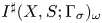 $I^{\sharp }(X,S;\Gamma _{\sigma })_{\omega }$ induced by cobordisms to include also the case that
 $S$ is a normally immersed surface in
 $X$. Our approach in the present paper is a slight variant of what was done in the two previous cited papers: what we will do here is better adapted to the case of an unoriented surface
 $S$.
So, let  $f : S \looparrowright X$ be an ‘immersed cobordism’ from
 $(Y_{0}, K_{0})$ to
 $(Y_{1}, K_{1})$. We always assume, as in [Reference Kronheimer and MrowkaKM11], that
 $f$ has only transverse double points, and that these are in the interior of
 $X$. That is, the surface is normally immersed. We also assume that the double points do not lie on the surface
 $\omega$ which represents
 $w_{2}$. We do not want to orient
 $S$, and we therefore do not give a sign
 ${\pm }1$ to the double points of the immersion. At a double point
 $x\in f(S)$, we may choose the metric on
 $X$ so that the two branches of the immersion have orthogonal tangent planes,
 $\pi$ and
 $\pi '$, in
 $T_{x}X$. There are then exactly two complex structures
 $J$ and
 $-J$ on
 $T_{x}X$ such that:
(i) the complex structure is compatible with the metric and orientation of
$T_{x}X$;(ii)
$\pi$ and $\pi '$ are $J$-invariant.


The blow-ups of  $X$ at
 $x$ with respect to the complex structures
 $J$ and
 $-J$ are canonically identified: in both blow-ups, the exceptional set
 $\epsilon \subset \tilde {X}$ is the set of
 $J$-invariant 2-planes in
 $T_{x}X$. When identified with
 $\mathbb{C}\mathbb{P}^{1}$, however, the complex orientation of the exceptional set is different in the two cases. The proper transform
 $\tilde {f} : \tilde {S} \looparrowright \tilde {X}$ has one fewer double point than
 $f$.
In the above situation, we define  $I^{\sharp }(X, S ; \Gamma )_{\omega }$ for the immersed cobordism by requiring that
 \begin{equation} I^{\sharp}\big(X, S ; \Gamma_{\sigma}\big)_{\omega} = I^{\sharp}\big(\tilde{X}, \tilde{S} ; \Gamma_{\sigma}\big)_{\omega} + I^{\sharp}\big(\tilde{X}, \tilde{S} ; \Gamma_{\sigma}\big)_{\omega+\epsilon}. \end{equation}
On the right, we see the proper transform, equipped with two different Stiefel–Whitney classes, differing by the exceptional set  $\epsilon$ of the blow-up. By applying the definition to each double point in turn, we arrive at a definition that reduces to the standard case of embedded cobordisms.
Before proceeding further, we make some remarks about this definition. The proper transform is being used here to construct a functor from a category in which the morphisms are immersed cobordisms to one in which the morphisms are embedded cobordisms. In the previous papers [Reference Kronheimer and MrowkaKM11, Reference Kronheimer and MrowkaKM13, Reference KronheimerKro97], such a construction was used with only the first of the two terms on the right. The reason for using the two terms, involving both  $\omega$ and
 $\omega +\epsilon$, is to provide a deformation invariance that would otherwise be absent, in the case that
 $\omega$ has boundary on
 $S$. To understand this, consider a local model for a double point of
 $S$, consisting of a pair of disks
 $D_{1}\cup D_{2}$ in the product
 $D_{1}\times D_{2}$, and let coordinates
 $(x_{i}, y_{i})$ be standard coordinates on
 $D_{i}$, so that the disks meet at the origin. Let
 $\omega$ be described in this neighborhood by
 \[ \omega = \{y_{1} = 1/2, \; y_{2} = 0, \; x_{2}\ge 0\}, \]
so that  $\partial \omega$ is the line
 $y_{1}=1/2$ on the disk
 $D_{1}$. Let
 $\omega '$ be obtained from
 $\omega$ by deforming
 $\omega$ in this neighborhood in such a way that (i)
 $\partial \omega '$ is the line
 $y=-1/2$ on
 $D_{1}$; and (ii)
 $\omega '$ intersects
 $D_{2}$ transversely at a point. Let
 $(\tilde {X}, \tilde {S}$ be obtained by blowing up the double point
 $D_{1}\cap D_{2}$, and regard
 $\omega$,
 $\omega '$ as lying in
 $\tilde {X}$. In this situation (assuming that this local picture is just part of cobordism of pairs), we have
 \[ I^{\sharp}(\tilde{X}, \tilde{S} ; \Gamma_{\sigma})_{\omega} \ne I^{\sharp}(\tilde{X}, \tilde{S} ; \Gamma_{\sigma})_{\omega'} \]
in general, because  $\omega$ and
 $\omega '$ are representatives of Stiefel–Whitney classes of different orbifold bundles. Instead, we have
 \[ I^{\sharp}(\tilde{X}, \tilde{S} ; \Gamma_{\sigma})_{\omega} = I^{\sharp}(\tilde{X}, \tilde{S} ; \Gamma_{\sigma})_{\omega'+\epsilon} \]
and similarly
 \[ I^{\sharp}(\tilde{X}, \tilde{S} ; \Gamma_{\sigma})_{\omega+\epsilon} = I^{\sharp}(\tilde{X}, \tilde{S} ; \Gamma_{\sigma})_{\omega'}. \]
So, if we wish to define 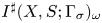 $I^{\sharp }( X, S ; \Gamma _{\sigma })_{\omega }$ when
 $S$ is normally immersed, and if we wish the result to be independent of the choice of
 $\omega$, in this way, we should take the two terms together, as we have done in (34).
With that said, if we impose the restriction that we consider only  $\omega$ without boundary along
 $S$, then we are free to modify the definition of the functor: for any fixed choice of
 $\xi \in \mathcal {S}$, we can define a functor
 $I^{\sharp }_{\xi }$ by leaving everything unchanged except for the rule for dealing with double points, where we substitute the variant
 \begin{equation} I^{\sharp}_{\xi}\big(X, S ; \Gamma_{\sigma}\big)_{\omega} = I^{\sharp}_{\xi}\big(\tilde{X}, \tilde{S} ; \Gamma_{\sigma}\big)_{\omega} + \xi \,I^{\sharp}_{\xi}\big(\tilde{X}, \tilde{S} ; \Gamma_{\sigma}\big)_{\omega+\epsilon}. \end{equation}
For the rest of this paper, we shall remain with the more restricted case  $\xi =1$, with only occasional comments about the more general version.
4.4 Twist moves and finger moves
We now follow the strategy from [Reference Kronheimer and MrowkaKM11] to see how  $I^{\sharp }(X, S ; \Gamma _{\sigma })$ changes when the immersion is changed in three standard ways (introducing additional double points). These are the ‘twist move’, which comes in two oriented flavors, and the ‘finger move’.
Proposition 4.4 (cf. [Reference Kronheimer and MrowkaKM11, Proposition 5.2] and [Reference Kronheimer and MrowkaKM13, Proposition 3.1])
Let  $S^{*}$ be obtained from
 $S$ by either a positive twist move or a finger move (introducing a canceling pair of double points). Then we have
 \[ I^{\sharp}(X, S^{*} ; \Gamma_{\sigma})_{\omega} = \sigma(L)\, I^{\sharp}(X, S ; \Gamma_{\sigma})_{\omega}, \]
where
 \[ L = P + T_{0}^{2} + T_{0}^{{-}2}. \]
For the negative twist move, on the other hand, the map  $I^{\sharp }$ is unchanged:
 \[ I^{\sharp}(X, S^{*} ; \Gamma_{\sigma})_{\omega} = I^{\sharp}(X, S ; \Gamma_{\sigma})_{\omega}. \]
Remark If we put  $T_{1}=T_{2}=T_{3} = 1$, the formulae in the above proposition are essentially the same as those in [Reference Kronheimer and MrowkaKM11, Proposition 5.2], but with the ‘
 $t$’ from that earlier paper now replaced by
 $T_{0}^{2}$. The factor of
 $2$ in the exponent again arises because we have used the
 $\mathop {{SO}}(3)$ connection rather than the
 $\mathop {{SU}}\nolimits (2)$ connection in defining the local system. Formulae of this sort go back to [Reference KronheimerKro97]. The case of the finger move is also formally similar to crossing-change results in Heegaard–Floer homology [Reference Ozsváth, Stipsicz and SzabóOSS15, Reference Alishahi and EftekharyAE20] and in Bar-Natan homology [Reference AlishahiAli19].
We prove the various parts of this proposition in the paragraphs. Our exposition describes just the case of  $\Gamma$, because the results are local, and the general
 $\Gamma _{\sigma }$ is obtained by base change.
4.4.1 Twist moves
We begin with the positive twist move. In this case, as explained in [Reference Kronheimer and MrowkaKM11] and [Reference KronheimerKro97], the result of the positive twist move followed by taking the proper transform in the blow-up is to replace  $(X,S)$ with
 \[ (X' , S') = (X, S) \mathbin{\#} (\overline{\mathbb{C}\mathbb{P}}^{2} , C), \]
where  $C$ is a smooth conic curve. According to our definition (34), we must therefore compute
 \[ I^{\sharp}(X', S' ; \Gamma)_{\omega} + I^{\sharp}(X', S' ; \Gamma)_{\omega+\epsilon}. \]
Once again, we compute by a connected-sum argument. A dimension count shows that the weak limit  $[E,A]$ on
 $(\overline {\mathbb{C}\mathbb{P}}^{2} , C)$ lies in a moduli space of formal dimension
 $d_{0} \le -1$, which means that its action
 $\kappa _{0}$ satisfies the bound
 $\kappa _{0} \le 1/4$. Since the formal dimension is negative, the connection must be reducible, to
 $\pm 1$, to
 $\mathop {{SO}}(2)$ or to
 $O(2)$. The double cover is
 $S^{2}\times S^{2}$, with the involution
 $\tau (x,y) = (-y,-x)$. The fixed-point set is the anti-diagonal
 $\Delta ^{-}$. The pull-back
 $[\tilde {E}, \tilde {A}]$ on
 $S^{2}\times S^{2}$ must be reducible, either to
 $\mathop {{SO}}(2)$ or to the trivial group, so this
 $\mathop {{SO}}(3)$ bundle has the form
 \[ \mathbb{R} \oplus K, \]
where  $e(K)$ can be taken to be
 $\tau$-invariant in the case that
 $[E,A]$ reduces to
 ${\pm }1$, and
 $\tau$-anti-invariant in the case that
 $[E,A]$ reduces to
 $O(2)$. In the standard basis,
 $e(K)$ has the form
 $(\delta , -\delta )$ or
 $(\delta , \delta )$, respectively. A class of the second sort is not represented by an anti-self-dual form, however. So,
 $e(K)=(\delta , -\delta )$ and
 $[E,A]$ reduces either to
 $\pm 1$ or to
 $\mathop {{SO}}(2)$. The bound on
 $\kappa _{0}$ means that
 $e(K)^{2} \ge -2$, so
 $\delta ^{2}\le 1$.
If  $\delta =0$, then
 $w_{2}(\tilde {E}) = 0$, which means that
 $w_{2}(E) = \epsilon$ in the neighborhood of the blow-up. If
 $\delta =\pm 1$, then
 $w_{2}(E)$ is zero in the neighborhood. The dimension count shows that the two cases
 $\delta ={\pm }1$ are unobstructed, and these contribute the terms
 $T_{0}^{2} + T_{0}^{-2}$. (The calculation here is just as in [Reference Kronheimer and MrowkaKM11].) So, we have
 \[ I^{\sharp}(X', S' ; \Gamma)_{\omega} = (T_{0}^{2} + T_{0}^{{-}2}) I^{\sharp}(X, S ; \Gamma)_{\omega}. \]
The case  $\delta =0$ is the case of the flat bifold connection on
 $(\overline {\mathbb{C}\mathbb{P}}^{2}, C)$ and it contributes to the term
 $I^{\sharp }( X', S' ; \Gamma )_{\omega +\epsilon }$. The obstruction space is again two dimensional, and just as the case of a connected sum with either
 $(S^{4}, R_{-})$ or
 $(S^{4}, T^{2})$, we obtain
 \[ I^{\sharp}(X', S' ; \Gamma)_{\omega+\epsilon} = P I^{\sharp}(X, S ; \Gamma)_{\omega}. \]
This concludes the proof for the positive twist move.
The negative twist move is straightforward. In this case we must consider  $(X', S')$ obtained from
 $(X,S)$ by forming the connect sum with
 $(\overline {\mathbb{C}\mathbb{P}}^{2}, \emptyset )$. The term with
 $\epsilon$ does not contribute, and the term
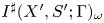 $I^{\sharp }(X', S' ; \Gamma )_{\omega }$ is equal to
 $I^{\sharp }(X, S ; \Gamma )_{\omega }$ as in [Reference Kronheimer and MrowkaKM11].
4.4.2 Finger moves
Let  $S^{*}$ be obtained from
 $S$ by a finger move, and let
 $S'$ be obtained from
 $S^{*}$ by blowing up at the two double points and taking the proper transform. Let
 $\epsilon _{1}$ and
 $\epsilon _{2}$ be the exceptional sets of the two blow-ups. From the definition in (34), we see that what we must compute is a sum of four terms
 \begin{equation} \mathop{{I}}\nolimits^{\sharp}(X', S' ; \Gamma)_{\omega} + \mathop{{I}}\nolimits^{\sharp}(X', S' ; \Gamma)_{\omega + \epsilon_{1}} + \mathop{{I}}\nolimits^{\sharp}(X', S' ; \Gamma)_{\omega + \epsilon_{2}} + \mathop{{I}}\nolimits^{\sharp}(X', S' ; \Gamma)_{\omega + \epsilon_{1} + \epsilon_{2}} \end{equation}
and the desired answer is 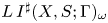 $L \,I^{\sharp }(X, S; \Gamma )_{\omega }$, where
 $L$ is as in the proposition.
To focus on the region where the change occurs, let us write
 \[ (X,S) = (X_{1}, S_{1}) \cup (X_{2}, S_{2}), \]
where  $(X_{2}, S_{2})$ is a standard 4-ball containing a standard pair of disks, and
 $(X_{1}, S_{1})$ is the closure of the complement. The two pairs meet along a pair
 $(S^{3}, U_{2})$, where
 $U_{2}\subset$ is a standard two-component unlink. Let
 $(X_{2}', S_{2}')$ be obtained from
 $(X_{2}, S_{2})$ by the finger move and proper transform. So, we have
 \[ (X', S') = (X_{1}, S_{1}) \cup (X_{2}' , S_{2}'). \]
The manifold  $(X_{2}' , S_{2}')$ has boundary
 $(S^{3}, U_{2})$, and we can form from it a closed pair by attaching a 4-ball and a standard pair of disks. We write
 $(Z, \Sigma )$ for the resulting pair:
 \begin{equation} (Z, \Sigma) = \big(X_{2}', S_{2}'\big) \cup \big(B^{4}, D^{2}\amalg D^{2}\big). \end{equation}
The manifold  $Z$ is a connected sum of two copies of
 $\overline {\mathbb{C}\mathbb{P}}^{2}$, and we write
 $E_{1}$,
 $E_{2}$ for the two exceptional curves. The surface
 $\Sigma$ is a union of two spheres,
 \[ \Sigma = \Sigma_{1} \amalg \Sigma_{2}, \]
each of which has square  $-2$. The two components
 $\Sigma _{1}$ and
 $\Sigma _{2}$ have the same mod-2 homology class, but over the integers we have (depending on choices made)
 \begin{align*} [\Sigma_{1}] &={-} [E_{1}] - [E_{2}],\\ [\Sigma_{2}] &={-} [E_{1}] + [E_{2}]. \end{align*}
The proof of the formula for the finger move depends on understanding the moduli spaces on  $(Z,\Sigma )$ for small energy
 $\kappa$, namely
 $\kappa =0$ and
 $\kappa =1/4$. As in (36) above, we will need to understand these moduli spaces
 \[ M(Z,\Sigma)_{\nu} \]
for four different values of the Stiefel–Whitney class  $\nu$, namely
 \[ \nu = 0, \quad \nu =\epsilon_{1}, \quad \nu =\epsilon_{2} \quad \text{and}\quad \nu =\epsilon_{1} + \epsilon_{2}, \]
where  $\epsilon _{i}$ is a representative in the class of
 $E_{i}$. Let us write
 \[ M(Z, \Sigma)_{*} \]
for the union of  $M(Z,\Sigma )_{\nu }$ over these four values of
 $\nu$.
Because we are working with  $I^{\sharp }$, our interpretation of
 $M(Z,\Sigma )_{*}$ is that it parametrizes
 $\mathop {{SU}}\nolimits (2)$ gauge equivalence classes of anti-self-dual
 $\mathop {{SU}}\nolimits (2)$ connections on the complement of the four spheres
 $E_{1}$,
 $E_{2}$,
 $\Sigma _{1}$ and
 $\Sigma _{2}$, such that the limiting holonomy around the links of the spheres
 $\Sigma _{i}$ is order 4, and the holonomy around the links of the spheres
 $E_{i}$ are each
 $1$ or
 $-1$, depending on the value of
 $\nu$. The metric on
 $Z$ is an orbifold metric as usual, with singular set
 $\Sigma$.
Consider a flat line bundle  $\xi$ on
 \[ Z' = Z{\setminus} \big( \Sigma_{1}, \Sigma_{2}, E_{1}, E_{2}\big). \]
Write 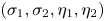 $(\sigma _{1}, \sigma _{2}, \eta _{1}, \eta _{2})$ for the holonomy of
 $\xi$ around the links of these four spheres, and require that these are
 $({\pm }1, {\pm }1, {\pm }1, {\pm }1)$. A push-off of
 $E_{1}$ meets
 $\Sigma _{1}$,
 $\Sigma _{2}$ and
 $E_{1}$ once each. Similarly with
 $E_{2}$. So,we have relations
 \[ \eta_{1}= \eta_{2} = \sigma_{1} + \sigma_{2}. \]
So, there are four possibilities for  $\xi$, including the trivial bundle, and their possible holonomies are
 \begin{align*} (\sigma_{1}, \sigma_{2}, \eta_{1}, \eta_{2}) & = (1,1,1,1), \quad\text{or} \\ & = (1,-1,-1,-1), \quad\text{or} \\ & = ({-}1,1,-1,-1), \quad\text{or} \\ & = ({-}1,-1,1,1). \end{align*}
They form the group isomorphic to  $V_{4}$.
The flat line bundles act  $\xi$ act on
 $M(Z,\Sigma )_{*}$ by tensor product. So, we have an action of
 $V_{4}$ on this moduli space. Tensoring by
 $\xi$ either leaves
 $\nu$ unchanged (if
 $\sigma _{1}=\sigma _{2}$) or adds
 $\epsilon _{1} + \epsilon _{2}$. So, the subset
 \begin{equation} M(Z,\Sigma)_{0} \cup M(Z,\Sigma)_{\epsilon_{1} + \epsilon_{2}} \end{equation}
is closed under the Klein 4-group action, as is the complementary subset,
 \begin{equation} M(Z,\Sigma)_{\epsilon_{1}} \cup M(Z,\Sigma)_{\epsilon_{2}}. \end{equation}
The quotient
 \[ M(Z,\Sigma)_{*} / V_{4} \]
parametrizes  $\mathop {{SO}}(3)$ anti-self-dual connections
 $[B]$ on the complement of the four spheres with the property that the holonomy around the links of the
 $\Sigma _{i}$ has order
 $2$ and the holonomy around the links of the
 $E_{i}$ is
 $1$ in
 $\mathop {{SO}}(3)$. This is the same as the space of bifold
 $\mathop {{SO}}(3)$ connections (without marking) on
 $(Z,\Sigma )$:
 \[ M(Z,\Sigma)_{*} / V_{4} = M_{\mathop{{SO}}(3)}(Z,\Sigma). \]
The next lemma (and the notation ‘twisted reducibles’) is from [Reference Kronheimer and MrowkaKM95].
Lemma 4.5 The action of the Klein 4-group is free except at ‘twisted reducibles’. That is, the  $\mathop {{SU}}\nolimits (2)$ connection
 $A$ is gauge equivalent to
 $A\otimes \xi$ if and only if the holonomy of
 $[\mathrm {ad}(A)]$ is contained in
 $O(2)\subset \mathop {{SO}}(3)$ and the associated real line bundle to the
 $O(2)$ connection is isomorphic to
 $\xi$.
The situation described in the lemma above can happen only if  $\xi$ either trivial or has
 \[ \big(\sigma_{1}, \sigma_{2}, \eta_{1}, \eta_{2}\big) =({-}1,-1,1,1). \]
We are now ready to describe the small-action moduli spaces, beginning with a description of the quotients 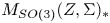 $M_{\mathop {{SO}}(3)}(Z,\Sigma )_{*}$.
Lemma 4.6 The space of bifold connections 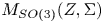 $M_{\mathop {{SO}}(3)}(Z,\Sigma )$ with
 $\kappa =0$ consists of a single point, with
 $\mathbb{Z}/2$ monodromy and
 $O(2)$ stabilizer.
For generic metrics, the space of bifold connections 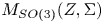 $M_{\mathop {{SO}}(3)}(Z,\Sigma )$ with
 $\kappa =1/4$ consists of a single arc and possibly some additional circles. Except for the end points of the arc, these bifold connections with
 $\kappa =1/4$ are irreducible (i.e. have trivial stabilizer in
 $\mathop {{SO}}(3)$). The end points of the arc have
 $\mathop {{SO}}(2)$ holonomy and therefore
 $\mathop {{SO}}(2)$ stabilizer.
Proof. For  $\kappa =0$, we are looking at flat orbifold bundles, or
 $\mathop {{SO}}(3)$ representations of the orbifold fundamental group. The fundamental group of
 $Z{\setminus} \Sigma$ is
 $\mathbb{Z}/2$, because this space is
 $(0,1)\times \mathop {\mathbb{R}\mathbb{P}}\nolimits ^{3}$. The two links of
 $S$ are non-zero elements. So, there is a unique bifold connection.
For  $\kappa =1/4$, consider the branched double cover of
 $\tilde {Z} \to Z$ along
 $\Sigma$. Let
 $\tilde {\Sigma }$ be the inverse image of
 $\Sigma$. This consists of two spheres
 $\tilde {\Sigma }_{i}$, each of self-intersection
 $-1$. The manifold
 $\tilde {Z}$ itself is diffeomorphic to a connected sum of two copies of
 $\overline {\mathbb{C}\mathbb{P}}^{2}$. On
 $\tilde {Z}$, we seek
 $\mathop {{SO}}(3)$ connections with action
 $\tilde \kappa =1/2$, which requires
 $w_{2}^{2} = 2$ mod
 $4$. So,
 $w_{2}=(1,1)$ in the standard basis. This is the sort of one-dimensional moduli space considered in [Reference Fintushel and SternFS84], from which we learn that the moduli space on
 $\tilde {Z}$ with
 $w_{2}=(1,1)$ and
 $\kappa =1/2$ is one dimensional and compact. Its end points correspond to pairs of integer classes
 $\pm \lambda$ where
 $\lambda ^{2}=-2$ and
 $\lambda =w_{2}$ mod
 $2$. The only possibilities are
 $\pm (1,1)$ and
 $\pm (1,-1)$. So, the moduli space has two end points. The end points correspond to reducible connections.
Returning to  $Z$, the covering transformation preserves the classes
 $\lambda =(1,1)$ and
 $(1,-1)$, so the corresponding
 $\mathop {{SO}}(2)$ connections on
 $\tilde {Z}$ descend to
 $\mathop {{SO}}(2)$ connections on
 $Z$. The moduli space on
 $Z$ is one dimensional, so must include an arc joining these two points. That is, the arc which is contained in the moduli space of
 $\tilde {Z}$ consists of invariant connections which descend to
 $Z$.
Lemma 4.5, together with the description of the  $\mathop {{SO}}(3)$ moduli space in last lemma above, gives us a description of the low-dimensional parts of
 $M(Z,\Sigma )_{*}$.
Proposition 4.7 The  $\kappa =0$ part of
 $M(Z,\Sigma )_{*}$ consists of two points, each of which has monodromy group the cyclic group
 $\langle \mathbf {i} \rangle \subset \mathop {{SU}}\nolimits (2)$ of order
 $4$. Under the Klein 4-group action (tensoring by flat line bundles), these are each fixed up to gauge equivalence by the action of tensoring by the line bundle
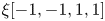 $\xi [-1,-1,1,1]$ (in the obvious notation from above). The two connections are interchanged by tensoring with
 $\xi [1,-1,-1,-1]$. These two points belong to the moduli spaces
 $M(Z,\Sigma )_{\epsilon _{1}}$ and
 $M(Z, \Sigma )_{\epsilon _{2}}$.
The  $\kappa =1/4$ part of
 $M(Z,\Sigma )_{*}$ consists of four arcs, together perhaps with some circles. The Klein 4-group acts transitively on the four arc components of the moduli space. Two of the arcs belong to
 $M(Z,\Sigma )_{0}$ and two belong to
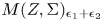 $M(Z,\Sigma )_{\epsilon _{1}+\epsilon _{2}}$.
Proof. From the previous lemma, the  $\kappa =0$ part of the moduli space
 $M(Z,\Sigma )_{*}$ consists of a single orbit of
 $V_{4}$. From Lemma 4.5, we also learn that the stabilizer of the orbit is the two-element subgroup consisting of the trivial line bundle and the line bundle
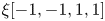 $\xi [-1,-1,1,1]$. Since the fundamental group of the complement of
 $\Sigma$ is
 $\mathbb{Z}/2$, there is no flat
 $\mathop {{SU}}\nolimits (2)$ bundle on
 $Z{\setminus} \Sigma$ whose holonomy on the links of
 $\Sigma$ is conjugate to the element
 $\mathbf {i}$ of order
 $4$. So, the flat
 $\mathop {{SU}}\nolimits (2)$ connection exists only on
 $Z{\setminus} (\Sigma \cup E_{1} \cup E_{2})$ and must have holonomy
 $-1$ on the link of exactly one
 $E_{i}$. These flat connections therefore belong to
 $M(Z,\Sigma )_{\epsilon _{1}}$ and
 $M(Z,\Sigma )_{\epsilon _{2}}$.
We now turn to the  $\kappa =1/4$ part of the moduli space. The previous lemmas again tell us that the Klein 4-group acts freely and the quotient is a 1-manifold containing a single arc. Therefore,
 $M(Z,\Sigma )_{*}$ contains four arcs. We are left to determine which of the four parts of
 $M(Z,\Sigma )_{\nu }$ (
 $\nu =*$) these belong to. An instanton
 $[A] \in M(Z,\Sigma )_{*}$ belonging to one of these arcs pulls back to an
 $\mathop {{SU}}\nolimits (2)$ instanton
 $[\tilde {A}]$ on
 \[ \tilde{Z} {\setminus} \big(\tilde{\Sigma} \cup \tilde{E}_{1} \cup \tilde{E}_{2}\big) \]
with limiting holonomy  $-1$ on the links of
 $\tilde {\Sigma }$. The limiting holonomy on the links of the sphere
 $\tilde {E}_{i}$ will be
 $(-1)^{\delta _{i}}$, where
 $\delta _{i}=1$ or
 $0$ according to whether
 $\epsilon _{i}$ appears in
 $\nu$. Because
 $[\tilde {E}_{i}]=[\tilde {\Sigma }_{1}]+[\tilde {\Sigma }_{2}]$ in mod-2 homology, we then obtain
 \[ w_{2}( \mathrm{ad}(\tilde{A}) ) = (1 + \delta_{1}+\delta_{2})([\tilde{\Sigma}_{1}] + [\tilde{\Sigma}_{2}]). \]
However, the previous lemma tells us that the Stiefel–Whitney class of  $[\mathrm {ad}(\tilde {A})]$ is dual to
 $[\tilde {\Sigma }_{1}]+[\tilde {\Sigma }_{2}]$. Therefore, the possibilities are only
 $(\delta _{1}, \delta _{2})=(0,0)$ or
 $(1,1)$. The four arcs therefore belong to the components
 $M(Z,\Sigma )_{0}$ and
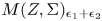 $M(Z,\Sigma )_{\epsilon _{1}+\epsilon _{2}}$. Two lie in each, because of the symmetry that arises from the
 $V_{4}$ action.
Corollary 4.8 If  $A$ and
 $A'$ are the two (abelian) connections which comprise the zero-dimensional part of
 $M(Z,\Sigma )_{*}$, and if
 $m_{1}$ and
 $m_{2}$ are links of the two components of
 $\Sigma$, oriented so that
 $A$ has monodromy
 $\mathbf {i}$ around both links, then the monodromies of
 $A'$ around
 $m_{1}$ and
 $m_{2}$ are
 $\mathbf {i}$ and
 $-\mathbf {i}$, up to overall conjugacy.
Let us return now to the pair  $(X'_{2}, \Sigma '_{2})$, which we equip with a cylindrical end
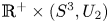 $\mathbb{R}^{+}\times (S^{3}, U_{2})$. With notation adapted from the discussion of
 $(Z,\Sigma )$, we examine the moduli space
 \[ M(X'_{2}, S'_{2})_{*} \]
on the cylindrical end moduli spaces, with Stiefel–Whitney class  $\nu =*$ running over the same four values. The
 $\mathop {{SU}}\nolimits (2)$ representation variety of
 $(S^{3}, U_{2})$ is an interval, which we denote by
 $[-1,1]$, so we have a map
 \[ r : M(X'_{2}, S'_{2})_{*} \to [{-}1,1]. \]
From Proposition 4.7 and a stretching argument, we learn that the  $\kappa =0$ part
 $M(X'_{2}, S'_{2})_{*}$ consists of two points which are mapped by
 $r$ to end points of the interval
 $[-1,1]$. From Corollary 4.8 we learn that the two points map to opposite ends of the moduli space.
Similarly, we learn that the  $\kappa =1/4$ part of
 $M(X'_{2}, S'_{2})_{*}$ contains four arcs, and that these are each mapped to
 $[-1,1]$ in such a way that the two end points of each arc map to opposite ends of
 $[-1,1]$.
Having described these moduli spaces on the cylindrical-end manifold, we now describe how these give rise to the formula in Proposition 4.4 for the case of the finger move. We can break the formula up into:
(i) terms coming from the classes
$\nu =0$ and $\nu =(\epsilon _{1} + \epsilon _{2})$ on the one hand; and(ii) terms coming from the classes
$\nu =\epsilon _{1}$ and $\nu =\epsilon _{2}$


(cf. (38) and (39) above). The first case is that of the four arcs that comprise the  $\kappa =1/4$ moduli space. Here the discussion closely mirrors the argument for the finger move in [Reference KronheimerKro97] and [Reference Kronheimer and MrowkaKM11]. Each of the four arcs will contribute a term to the formula having the shape
 \[ T_{0}^{x} T_{0}^{y} I^{\sharp}(X, S; \Gamma)_{\omega}, \]
where  $x$ and
 $y$ are curvature integrals for
 $\mathop {{SO}}(2)$ connections on the components
 $\Sigma '_{1}$,
 $\Sigma '_{2}$ of the singular set in the cylindrical-end bifold
 $(X_{2}',S'_{2})$. The action of the group
 $V_{4}$ is by tensoring with real line bundles, the effect of which is to change the signs of
 $x$ and
 $y$. So, the formula for the four arcs together has the form
 \[ \big( T_{0}^{x}T_{0}^{y} + T_{0}^{{-}x}T_{0}^{y} + T_{0}^{x}T_{0}^{{-}y} + T_{0}^{{-}x}T_{0}^{{-}y}\big) I^{\sharp}(X, S; \Gamma)_{\omega}. \]
By symmetry, we have  $x=y$ up to sign. So, the formula simplifies to
 \[ ( T_{0}^{2x} + T_{0}^{{-}2x}) I^{\sharp}(X, S; \Gamma)_{\omega}. \]
A special case of the finger move is a pair of twist moves, one positive and one negative. So, by comparing this formula to the case of the twist moves, we see that  $x=\pm 1$. So, the contribution of the
 $\kappa =1/4$ moduli spaces to the formula for
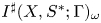 $I^{\sharp }(X,S^{*};\Gamma )_{\omega }$ is
 \begin{equation} ( T_{0}^{2} + T_{0}^{{-}2}) I^{\sharp}(X, S; \Gamma)_{\omega}. \end{equation}
Turning finally to the contributions from the classes  $\nu =\epsilon _{1}$ and
 $\nu =\epsilon _{2}$, we have seen that the
 $\kappa =0$ moduli spaces
 \[ M(X_{2}, S_{2}')_{\epsilon_{1}} \quad\text{and}\quad M(X_{2}, S_{2}')_{\epsilon_{2}} \]
each consist of a single point and these map to the two end points of  $[-1,1]$. We can compare this to the moduli space
 $M(X_{2}, S_{2})$ with
 $\kappa =0$ (where
 $(X_{2}, S_{2})$ is now a ball with two disks, equipped with a cylindrical end). For the latter moduli space, the map
 \[ r: M(X_{2}, S_{2})_{\kappa=0} \to [{-}1,1] \]
is a homeomorphism. Let us pick points  $p$ and
 $q$ on the two disks and orientations
 $o_{p}$ and
 $o_{q}$ nearby. The flat connections on the orbifold
 $(X_{2}, S_{2})$ are determined by the holonomies around oriented meridians at this point, as in § 3.2, or equivalently by unit vectors
 $i_{p}$ and
 $i_{q}$ in the
 $\mathbb{R}^{3}$ fibers
 $\mathbb{E}_{p}$ and
 $\mathbb{E}_{q}$. Under the homeomorphism
 $r$, the end points of the interval correspond to flat connections with
 $i_{p}=i_{q}$ and
 $i_{p}=-i_{q}$ (when we identify
 $\mathbb{E}_{p}$ with
 $\mathbb{E}_{q}$ via paths to the base point). If we work with the based moduli space of flat connections on
 $(X_{2}, S_{2})$, then we instead obtain a map
 \[ r: \tilde{M}(X_{2},S_{2})_{\kappa=0} \to [{-}1,1], \]
where the domain is now  $S^{2}\times S^{2}$ and the preimage of the end points is the union of the diagonal and anti-diagonal. This is precisely the intersection of
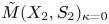 $\tilde {M}(X_{2},S_{2})_{\kappa =0}$ with the standard representatives of the two-dimensional cohomology classes
 $\lambda _{pq}$ and
 $\lambda '_{pq}$ from (27). If we recall the relation
 $\lambda _{pq} + \lambda '_{pq}= w_{2}(\mathbb{E}_{p})$ from Lemma 3.6, then we learn that the preimage of the two end points comprises a standard representative for the Poincaré dual of
 $w_{2}$. From Lemma 3.1 and a stretching argument, it then follows that for the original closed pair
 $(X,S)$ and the pair
 $(X,S^{*})$ obtained by the finger move, the contribution to
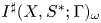 $I^{\sharp }(X,S^{*} ; \Gamma )_{\omega }$ coming from these moduli spaces is
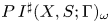 $P \, I^{\sharp }(X, S; \Gamma )_{\omega }$. This formula and the terms (40) together give the formula in Proposition 4.4 for the finger move:
 \begin{equation} I^{\sharp}(X, S^{*}; \Gamma)_{\omega} = ( P + T_{0}^{2} + T_{0}^{{-}2}) \,I^{\sharp}(X, S ; \Gamma)_{\omega} \end{equation}
or more succinctly
 \begin{equation} I^{\sharp}(X, S^{*}; \Gamma)_{\omega} =L \,I^{\sharp}(X, S ; \Gamma)_{\omega}. \end{equation}
Remark As discussed in § 4.3 above, we can choose to change our definition for the blow-ups and use the formula (35). A little extra book-keeping is then required, but the final result needs only slight modification. For the resulting functor  $I^{\sharp }_{\xi }$, the statement of Proposition 4.4 is unchanged except for the formula for the factor
 $L$. We record this as a proposition.
Proposition 4.9 As in Proposition 4.4, let  $S^{*}$ be obtained from
 $S$ by either a positive twist move or a finger move. Let the modified functor
 $I^{\sharp }_{\xi }$ be defined using the blow-up rule (34). Then we have
 \[ I^{\sharp}_{\xi}(X, S^{*} ; \Gamma_{\sigma})_{\omega} = \sigma(L_{\xi})\quad I^{\sharp}_{\xi}(X, S ; \Gamma_{\sigma})_{\omega}, \]
where
 \[ L_{\xi} = \xi P + T_{0}^{2} + T_{0}^{{-}2}. \]
For the negative twist move, the map  $I^{\sharp }_{\xi }$ is again unchanged:
 \[ I^{\sharp}(X, S^{*} ; \Gamma_{\sigma})_{\omega} = I^{\sharp}(X, S ; \Gamma_{\sigma})_{\omega}. \]
4.5 Regular homotopies
Recall that if  $f_{0}$ and
 $f_{1}$ are two smooth embeddings of a closed surface
 $S$ in a 4-manifold
 $X$, and if
 $f_{0} \simeq\, f_{1}$ as maps, then one can find a homotopy which is a composite of steps, each of which is one of:
– the introduction of a transverse double point by a twist move;
– the introduction of two transverse double points by a finger move;
– the inverse to one of the above; and
– an ambient isotopy.
The same applies to surfaces  $S$ which arise as cobordisms between knots or links, when the homotopy is relative to the boundary. As in [Reference KronheimerKro97, Reference Kronheimer and MrowkaKM11, Reference Kronheimer and MrowkaKM13], this observation can be combined with the formulae in Proposition 4.4, to obtain the following result (among others).
Proposition 4.10 Let  $S \subset \mathbb{R}^{4}$ be a closed embedded surface, not necessarily connected. Regard
 $S$ as a cobordism from the empty link in
 $\mathbb{R}^{3}$ to itself, optionally equipped with dots
 $q_{1}$,…,
 $q_d$. Then the resulting map
 \[ I^{\sharp}((S; q_{1}, \ldots, q_{d}) ; \Gamma_{\sigma}) : \mathcal{S} \to \mathcal{S} \]
depends only on the topology of the components of  $S$, the number of dots on each and the local orientations.
5. The unknot and unlinks
The instanton homology  $I^{\sharp }(K; \Gamma _{\sigma })$ is a free
 $\mathcal {S}$-module of rank
 $2$ when
 $K$ is the unknot, and it is a free module of rank
 $2^{n}$ for the
 $n$-component unlink. Although establishing these statements is not hard, we will need a little more for application in our spectral sequence in the following section: we need to make these isomorphisms canonical, to the extent that is possible. For this task, our exposition will follow [Reference Kronheimer and MrowkaKM12] to begin with. However, there is a little more subtlety now, even in the case of the unknot. This stems in part from the fact that
 $I^{\sharp }(K ;\Gamma )$ is only
 $\mathbb{Z}/2$ graded (there is no
 $\mathbb{Z}/4$ grading as there was in [Reference Kronheimer and MrowkaKM12]), and the two generators for the unknot are in the same grading mod
 $2$, so we cannot use the grading decomposition to pick out canonical generators.
5.1 Spheres with dots
Let  $S \subset \mathbb{R}^{4}$ be an embedded sphere. Choose one orientation and let
 $q_{1}, \ldots, q_{d}$ be dots on
 $S$ whose orientation agrees with the chosen orientation of
 $S$. We wish to evaluate the corresponding map on the homology of the empty link, which we regard as defining an element
 \[ I^{\sharp}((S; q_{1}, \ldots, q_{d}); \Gamma_{\sigma}) \in \mathcal{S}, \]
where  $\Gamma _{\sigma } = \Gamma \otimes _{\sigma } \mathcal {S}$. By Proposition 4.10, the evaluation is independent of the embedding.
Lemma 5.1 The evaluation  $\epsilon _{d}$ of the sphere with
 $d$ dots is
 $0$ for
 $d=0$, and
 $1$ for
 $d=1$. For
 $d\ge 2$, it satisfies the recurrence relation
 \[ \epsilon_{d} = \sigma(P) \epsilon_{d-1} + \sigma(Q) \epsilon_{d-2}. \]
Proof. The formal dimension of the relevant moduli space is positive when the Yang–Mills action  $\kappa$ is zero, so for
 $d=0$ the evaluation is zero. For
 $d=1$, we use the fact that the
 $\kappa =0$ moduli space parametrizes flat connections and is a
 $2$-sphere when
 $S$ has the standard embedding. The cohomology class
 $\lambda _{q}$ is set up so that it evaluates to
 $1$ on this
 $2$-sphere. For
 $d\ge 2$, the recurrence relation follows from Lemma 3.9.
5.2 The empty knot and the unknot
As in [Reference Kronheimer and MrowkaKM12], we write  $U_{n}$ for a standard unlink in
 $\mathbb{R}^{3}$ with
 $n$ components, so that
 $U_{0}$ is the empty link and
 $U_{1}$ is the unknot. We take
 $U_{n}$ to be the union of standard circles in the
 $(x,y)$ plane, each of diameter
 $1/2$, and centered on the first
 $n$ integer lattice points along the
 $x$ axis. We orient the circles of
 $U_{n}$ by a standard choice, say anti-clockwise in the
 $(x,y)$ plane.
For the empty link,  $I^{\sharp }(U_{0};\Gamma _{\sigma })$ is free of rank
 $1$ and we can canonically choose an identification with
 $\mathcal {S}$ or equivalently a generator
 \[ \mathbf{u}_{0} \in I^{\sharp}(U_{0};\Gamma_{\sigma}). \]
Lemma 5.2 For the unknot  $U_{1}$, the instanton homology
 $I^{\sharp }(U_{1}; \Gamma _{\sigma })$ is free of rank
 $2$. As generators, we can take the image of
 $\mathbf {u}_{0}$ under the two maps
 \[ I^{\sharp}(U_{0};\Gamma_{\sigma}) \to I^{\sharp}(U_{1};\Gamma_{\sigma}) \]
given by (a) a standard disk  $D^{+}$ with boundary
 $U_{1}$; or (b) the disk
 $D^{+}$ decorated with a dot
 $q$ whose local orientation arises from our choice of orientation for the knot.
Proof. The Chern–Simons functional has a perturbation with just two critical points. So, the rank is at most  $2$; and equality can hold only if it is a free module. Let
 $D^{-}$ be a disk providing a cobordism from
 $U_{1}$ to
 $U_{0}$ and let
 $q'$ be a dot on
 $D^{-}$. Using Lemma 5.1, we can compute the pairings between the cobordisms
 $D^{+}$,
 $(D^{+}, q)$ on the one side and the cobordisms
 $D^{-}$,
 $(D^{-}, q')$ on the other. The result is the matrix
 \[ \begin{pmatrix} 0 & 1 \\ 1 & P \end{pmatrix}, \]
whose determinant is  $1$. It follows that the rank of the module is
 $2$, the images of
 $D^{+}$ and
 $(D^{+}; q)$ are generators.
Definition 5.3 We write  $V$ for the rank-2
 $\mathcal {S}$-module
 $I^{\sharp }(U_{1}; \Gamma _{\sigma })$. Define
 \[ \mathbf{x}_{+}, \; \mathbf{x}_{-} \in I^{\sharp}(U_{1}; \Gamma_{\sigma}) \]
to be the images of  $\mathbf {u}_{0}$ under the maps arising from the cobordisms
 $D^{+}$ and
 $(D^{+}; q)$. They form a basis for this free module, by the lemma. In the dual module, we define
 \[ \mathbf{y}_{+} , \; \mathbf{y}_{-}: V \to \mathcal{S} \]
using respectively the cobordisms  $D^{-}$ and
 $(D^{-}, q)$.
The proof of the previous lemma gives the pairings between  $\mathbf {x}_{\pm }$ and
 $\mathbf {y}_{\pm }$, and from the knowledge of those pairings we obtain the following result.
Lemma 5.4 The dual basis to the basis  $(\mathbf {x}_{+}$,
 $\mathbf {x}_{-})$ for the free module
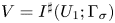 $V=I^{\sharp }(U_{1};\Gamma _{\sigma })$ is the basis
 $(\mathbf {y}_{-} + \sigma (P) \,\mathbf {y}_{+}, \mathbf {y}_{+})$.
5.3 The homology of the unlink
Having identified  $I^{\sharp }(U_{1}; \Gamma _{\sigma })$ as the free module
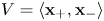 $V=\langle \mathbf {x}_{+}, \mathbf {x}_{-}\rangle$, we can examine the
 $n$-component unlink
 $U_{n}$ using the strategies from [Reference Kronheimer and MrowkaKM12].
Lemma 5.5 Corollary 8.5 of [Reference Kronheimer and MrowkaKM12]
We have an isomorphism of  $\mathcal {S}$-modules,
 \[ \Phi_{n}: V^{{\otimes} n} \to I^{\sharp}(U_{n};\Gamma_{\sigma}), \]
for all  $n$, with the following properties. First, if
 $D^{+}_{n}$ denotes the cobordism from
 $U_{0}$ to
 $U_{n}$ obtained from standard disks as in the previous lemma, then
 \[ I^{\sharp}(D^{+}_{n};\Gamma_{\sigma})(\mathbf{u}_{0}) = \Phi_{n}\big( \mathbf{x}_{+}\otimes \cdots \otimes \mathbf{x}_{+}\big). \]
Second, the isomorphism is natural for split cobordisms, perhaps with dots, from  $U_{n}$ to itself. Here, a ‘split’ cobordism means a cobordism from
 $U_{n}$ to
 $U_{n}$ in
 $[0,1]\times \mathbb{R}^{3}$ which is the disjoint union of
 $n$ cobordisms from
 $U_{1}$ to
 $U_{1}$, each contained in a standard ball
 $[0,1]\times B^{3}$.
Proof. This is essentially the same as the version in [Reference Kronheimer and MrowkaKM12]. Note that the trivial cobordism from  $U_{1}$ to
 $U_{1}$, equipped with a dot
 $q$ and an appropriate local orientation, gives the map
 $\Lambda _{q}:V\to V$ which maps
 $\mathbf {x}_{+}$ to
 $\mathbf {x}_{-}$.
The next lemma and its corollary are also drawn directly from [Reference Kronheimer and MrowkaKM12], and establish that the isomorphism of the previous lemma is canonical, once the unlink has been oriented.
Lemma 5.6 Let  $S$ be an oriented concordance from the standard unlink
 $U_{n}$ to itself, consisting of
 $n$ oriented annuli in
 $[0,1]\times \mathbb{R}^{3}$. Let
 $\tau$ be the permutation of
 $\{1,\ldots ,n\}$ corresponding to the permutation of the components of
 $U_{n}$ arising from
 $S$. Then the standard isomorphism
 $\Phi _{n}$ of Lemma 5.5 intertwines the map
 \[ I^{\sharp}(S;\Gamma_{\sigma}) : I^{\sharp}(U_{n};\Gamma_{\sigma}) \to I^{\sharp}(U_{n};\Gamma_{\sigma}) \]
with the permutation map
 \[ \tau_{*} : V\otimes \cdots\otimes V \to V\otimes \cdots \otimes V. \]
In particular, if the permutation  $\tau$ is the identity, then
 $I^{\sharp }(S;\Gamma _{\sigma })$ is the identity.
Proof. The proof leverages Proposition 4.10, and is the same as the proof in [Reference Kronheimer and MrowkaKM12], with the dot operator  $\Lambda _{q}$ replacing the operator
 $\sigma$ ((56) in [Reference Kronheimer and MrowkaKM12]).
Corollary 5.7 Let  $\mathcal {U}_{n}$ be any oriented link in the link type of
 $U_{n}$ and let its components be enumerated. Then there is a canonical isomorphism
 \[ \Psi_{n} : V\otimes \cdots \otimes V \to I^{\sharp}(\mathcal{U}_{n};\Gamma_{\sigma}) \]
which can be described as 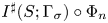 $I^{\sharp }(S;\Gamma _{\sigma }) \circ \Phi _{n}$, where
 $\Phi _{n}$ is the standard isomorphism of Lemma 5.5 and
 $S$ is any cobordism from
 $U_{n}$ to
 $\mathcal {U}_{n}$ arising from an isotopy from
 $U_{n}$ to
 $\mathcal {U}_{n}$, respecting the orientations and the enumeration of the components.
If the enumeration of the components of  $\mathcal {U}_{n}$ is changed by a permutation
 $\tau$, then the isomorphism
 $\Psi _{n}$ is changed simply by composition with the corresponding permutation of the factors in the tensor product.
The corollary tells us that the homology of the unlink is canonically isomorphic to the tensor product once an orientation of the components has been chosen. It is worth noting that the isomorphism does depend on the choice of orientation, as the following proposition shows.
Proposition 5.8 Let  $S: U_{1} \to U_{1}$ be a cobordism arising from an isotopy of the standard unknot to itself which reverses the orientation. Then the resulting map
 $\iota =I^{\sharp }(S; \Gamma _{\sigma }) : V \to V$ is given by
 \begin{align*} \iota : \mathbf{x}_{+} &\mapsto \mathbf{x}_{+}, \\ \iota : \mathbf{x}_{-} &\mapsto \sigma(P) \,\mathbf{x}_{+} + \mathbf{x}_{-}. \end{align*}
Proof. Recall that  $\mathbf {x}_{-}=\Lambda _{q}\mathbf {x}_{+}$. The cobordism
 $S$ intertwines the operator
 $\Lambda _{q}$ with
 $\Lambda '_{q}$. The formula for
 $\iota$ therefore follows from the relation
 $\Lambda _{q} + \Lambda _{q}'=\sigma (P)$ in Corollary 3.11.
5.4 Pants and copants
Recall the standard cobordism called ‘pants’, from the two-component unlink to the one-component unknot:
 \[ \mathord{\Pi}: U_{2} \to U_{1}. \]
Its mirror image is ‘copants’,
 \[ \mathord{\amalg}: U_{1} \to U_{2}. \]
If we identify  $I^{\sharp }(U_{1};\Gamma _{\sigma })$ and
 $I^{\sharp }(U_{2};\Gamma _{\sigma })$ with
 $V$ and
 $V\otimes V$ by the canonical isomorphisms of Corollary 5.7, then pants and copants give rise to maps
 \begin{equation} \begin{aligned} & I^{\sharp}(\mathord{\Pi}; \Gamma_{\sigma}) : V\otimes V \to V, \\ & I^{\sharp}(\mathord{\amalg}; \Gamma_{\sigma}) : V \to V\otimes V. \end{aligned} \end{equation}
Proposition 5.9 Under the above identification, the maps arising from the pants cobordism  $\mathord {\Pi }$ are given by
 \begin{equation} \begin{aligned} \mathbf{x}_{+} \otimes \mathbf{x}_{+} & \mapsto \mathbf{x}_{+}, \\ \mathbf{x}_{+} \otimes \mathbf{x}_{-} & \mapsto \mathbf{x}_{-}, \\ \mathbf{x}_{-} \otimes \mathbf{x}_{+} & \mapsto \mathbf{x}_{-}, \\ \mathbf{x}_{-} \otimes \mathbf{x}_{-} & \mapsto \sigma(P) \mathbf{x}_{-} + \sigma(Q) \mathbf{x}_{+}. \end{aligned} \end{equation}
The map arising from the copants cobordism  $\mathord {\amalg }$ is
 \begin{equation} \begin{aligned} \mathbf{x}_{+} & \mapsto \mathbf{x}_{+}\otimes \mathbf{x}_{-} + \mathbf{x}_{-}\otimes \mathbf{x}_{+} + \sigma( P)\mathbf{x}_{+}\otimes \mathbf{x}_{+},\\ \mathbf{x}_{-} & \mapsto \mathbf{x}_{-}\otimes \mathbf{x}_{-} + \sigma(Q) \mathbf{x}_{+} \otimes \mathbf{x}_{+}. \end{aligned} \end{equation}
Proof. Using the standard basis elements  $\mathbf {x}_{\pm }$ and dual basis
 $\mathbf {y}_{\pm }$, we can reduce this to the evaluation of a 2-sphere with dots, for which we have the formulae in Lemma 5.1.
5.5 The reduced homology of the unlink
Let  $\sigma : \mathcal {R}\to \mathcal {S}$ be a base change with
 $\sigma (T_{0})=\sigma (T_{1})$, so that the reduced instanton homology
 $I^{\natural }(K ; \Gamma _{\sigma })$ is defined for a link
 $K$ with base point. As with other ‘reduced’ versions of knot homologies, from the definitions,
 $I^{\natural }(U_{1} ; \Gamma _{\sigma }) \cong I^{\sharp }(U_{0}; \Gamma _{\sigma }) \cong \mathcal {S}$ and
 \begin{equation} \begin{aligned} I^{\natural}(U_{n}; \Gamma_{\sigma}) & \cong I^{\natural}(U_{1} ; \Gamma_{\sigma}) \otimes_{\mathcal{S}} I^{\sharp}(U_{n-1} ; \Gamma_{\sigma} )\\ & \cong I^{\sharp}(U_{n-1} ; \Gamma_{\sigma}). \end{aligned} \end{equation}
In particular,  $I^{\natural }(U_{n}; \Gamma _{\sigma })$ is a free module of rank
 $2^{n-1}$. We would like to compute the maps on
 $I^{\natural }(U_{n}; \Gamma _{\sigma })$ given by the pants and copants cobordisms, particularly when one the incoming components of the cobordisms carries the base point.
As a first step, we consider again the operator  $\Lambda _{q}$, for
 $q\in K$, now as an operator on
 $I^{\natural }(K;\Gamma _{\sigma })$. We define this as before, as in Definition 3.10,
 \[ \Lambda_{q} = \Lambda_{p_{1}q } + \Lambda_{p_{2}q } + \Lambda_{p_{3}q }, \]
where the three  $p_{i}$ are dots chosen near the vertex, so that
 $p_{2}$ and
 $p_{3}$ lie on the two edges that form the bigon in
 $K^{\natural }$.
If it happens that  $q$ lies on the component of
 $K$ where the bigon is attached, we can take
 $q=p_{1}$, in which case the first term
 $\Lambda _{p_{1}p_{1}}$ is
 $P$. In this setting, to compute the operator, it is sufficient to examine the case that
 $K$ is the unknot, by excision; so
 $K^{\natural }$ can be taken to be the theta graph. Each of the three terms is then an operator
 $\mathcal {S}\to \mathcal {S}$, so altogether
 $\Lambda _{q}$ is a multiplication operator,
 \[ \Lambda_{q} = A : \mathcal{S} \to \mathcal{S}. \]
To compute  $A$, we seek to compute
 \begin{equation} \Lambda_{q} = P + \Lambda_{p_{2} p_{1} } + \Lambda_{p_{3}p_{1} }. \end{equation}
The operator  $\Lambda _{p_{2}p_{1}}$ for the theta graph was computed in (31), up to a choice of two possibilities, differing by
 $P$. The same ambiguity is present twice in (47), for
 $\Lambda _{p_{2} p_{1} }$ and for
 $\Lambda _{p_{3} p_{1} }$, and it is resolved in the same way in both terms. So, the ambiguity cancels and we are left with a unique formula,
 \[ \Lambda_{q} = P + T_{3}\big(T_{1}T_{2} + T_{1}^{{-}1}T_{2}^{{-}1}\big) + T_{2}\big(T_{1}T_{3} + T_{1}^{{-}1}T_{3}^{{-}1}\big), \]
which simplifies to
 \[ A = T_{1} \big(T_{2}T_{3} + T_{2}^{{-}1}T_{3}^{{-}1}\big). \]
(We have omitted the base change  $\sigma$ in our notation.) To summarize this calculation in the case of the unknot, we have the following result.
Proposition 5.10 For the unknot  $U_{1}$, the reduced homology
 $I^{\natural }(U_{1}; \Gamma _{\sigma })$ is a free
 $\mathcal {S}$-module of rank
 $1$, on which the operator
 $\Lambda _{q}$ (
 $q\in U_{1}$) acts as multiplication by
 $A$, where
 $A$ is the element above.
What lies behind the algebra here is the following observation. The operator  $\Lambda$ on the un-reduced homology
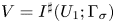 $V = I^{\sharp }(U_{1}; \Gamma _{\sigma })$ has minimum polynomial
 \[ x^{2} + \sigma(P)x + \sigma(Q). \]
When the base change has  $\sigma (T_{0})=\sigma (T_{1})$, the minimum polynomial factorizes as
 \[ (x + A)(x + A'), \]
where  $A$ is as above and
 $A'=A+P$. This is the same observation as we made in the introduction to this paper, at (11). Let us define
 $V^{\natural } \subset V$ as
 \begin{align*} V^{\natural} &= \ker( \Lambda+A) \\ &= \mathrm{im} (\Lambda+A'). \end{align*}
So,  $V^{\natural }$ is the rank-1
 $\mathcal {S}$-submodule generated by the element
 \[ \mathbf{m}=\mathbf{x}_{-} + A' \mathbf{x}_{+}. \]
Then we have the following result.
Corollary 5.11 The reduced homology  $I^{\natural }(U_{1}; \Gamma _{\sigma })$ is isomorphic as a module for
 $\mathcal {S}[\Lambda ]$ to the submodule
 $V^{\natural } \subset V$ generated by
 $\mathbf {m}$ above.
We can consider next the pants and copants cobordisms in the reduced context. Let  $U_{2}$ be the standard two-component unlink with a base point on the first component. We have, by excision,
 \[ I^{\natural}(U_{2} ;\Gamma_{\sigma}) = V^{\natural} \otimes_{\mathcal{S}} V. \]
The pants and copants cobordisms provide maps
 \begin{align*} I^{\natural}(\mathord{\Pi}; \Gamma_{\sigma}) : V^{\natural}\otimes V \to V^{\natural}, \\ I^{\natural}(\mathord{\amalg}; \Gamma_{\sigma}) : V^{\natural} \to V^{\natural} \otimes V. \end{align*}
It is straightforward to verify that these coincide with the restriction of the un-reduced versions (43) to the  $\mathcal {S}$-submodule
 $V^{\natural }$ generated by
 $\mathbf {m}$. We can write these maps out, in terms of the basis
 $\{ \mathbf {x}_{+}, \mathbf {m}\}$ for the rank-2
 $\mathcal {S}$-module
 $V$.
Proposition 5.12 When  $\sigma (T_{0})=\sigma (T_{1})$, so that the reduced theory is defined, the map
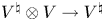 $V^{\natural }\otimes V \to V^{\natural }$ arising from the pants cobordism is
 \begin{equation} \begin{aligned} \mathbf{m} \otimes \mathbf{x}_{+} & \mapsto \mathbf{m}, \\ \mathbf{m} \otimes \mathbf{m} & \mapsto P \, \mathbf{m}. \end{aligned} \end{equation}
The map 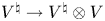 $V^{\natural }\to V^{\natural }\otimes V$ arising from copants is
 \begin{equation} \mathbf{m} \mapsto \mathbf{m} \otimes \mathbf{m}. \end{equation}
Returning again to  $V$ in the unreduced case, we have a description of it as an algebra over
 $\mathcal {R}$ with a single generator
 $\mathbf {n} = \mathbf {x}_{-}$ in the form
 \[ V = \mathcal{R}[\mathbf{n}] / (\mathbf{n}^{2} + P \mathbf{n} + Q). \]
As in the introduction, after a base change to a ring  $\mathcal {S}$ where
 $T_{0}=T_{1}$, the characteristic polynomial
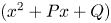 $(x^{2} + Px +Q)$ factorizes as
 $(x+A)(x+A')$ and over
 $\mathcal {S}$ we have a presentation
 \[ V = \mathcal{S}[\mathbf{m}] / (\mathbf{m}(\mathbf{m} + P)). \]
The full comultiplication of the Frobenius algebra  $V$, arising from the copants cobordism, in this presentation is
 \begin{align*} \Delta: \mathbf{1} &\mapsto \mathbf{m}\otimes \mathbf{1} + \mathbf{1}\otimes \mathbf{m} + P \mathbf{1}\otimes \mathbf{1}, \\ \Delta: \mathbf{m} &\mapsto \mathbf{m}\otimes\mathbf{m}. \end{align*}
This is the Frobenius algebra that gives rise to the graded Bar-Natan variant of Khovanov homology, tensored by  $\mathcal {S}$.
6. The spectral sequence
6.1 Families of metrics
Relevant to the construction of our spectral sequence are also the maps that arise from a cobordism equipped with a family of metrics. The material of [Reference Kronheimer and MrowkaKM12, § 3.9] again adapts to local coefficients without change. We equip  $(X,S)$ with cylindrical ends and a family of Riemannian metrics
 $G$ which vary only in a compact region. The parameter space
 $G$ should be a compact manifold with boundary. After choosing perturbations, the moduli spaces over
 $G$ define homomorphisms of
 $\mathcal {S}$-modules,
 \[ m_{G} : C^{\sharp}(Y_{0}, K_{0}; \Gamma_{\sigma}) \to C^{\sharp}(Y_{1}, K_{1}; \Gamma_{\sigma}), \]
where the complexes 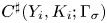 $C^{\sharp }(Y_{i}, K_{i}; \Gamma _{\sigma })$ are those that compute
 $I^{\sharp }$. The map
 $m_{G}$ is a chain map if
 $G$ has no boundary. Otherwise, there is an extra term in the chain formula,
 \[ m_{\partial G} + m_{G}\circ \partial = \partial \circ m_{G}. \]
(See [Reference Kronheimer and MrowkaKM12, § 3.9] and [Reference Kronheimer and MrowkaKM19a].)
6.2 Skein exact triangle
Fix again a  $3$-manifold
 $Y$ with base point
 $y_{0}$ and a theta graph
 $\theta \subset B(y_{0})$. We again write
 $Y^{o} \subset Y$ for the complement of the neighborhood of
 $y_{0}$. Consider three webs
 $K_{2}$,
 $K_{1}$,
 $K_{0}$ in
 $Y^{o}$ which are all identical outside a ball
 $B\subset Y^{o}$ and which differ inside
 $B$ by the skein moves as shown in Figure 4. There are standard cobordisms
 $S_{ij}$ from
 $K_{i}$ to
 $K_{j}$, each of which is the addition of a standard
 $1$-handle in
 $[0,1]\times B$. Although the webs may have vertices, there are no vertices in the ball
 $B$, and the picture coincides with that of [Reference Kronheimer and MrowkaKM12, § 6]. As in [Reference Kronheimer and MrowkaKM12, Reference Kronheimer and MrowkaKM19a], the cobordisms
 $S_{21}$,
 $S_{10}$ and
 $S_{02}$ give rise to the maps in a 3-periodic long exact sequence of
 $\mathcal {S}$-modules:
 \[ \cdots \to I^{\sharp}(K_{2}; \Gamma_{\sigma}) \to I^{\sharp}(K_{1}; \Gamma_{\sigma}) \to I^{\sharp}(K_{0}; \Gamma_{\sigma}) \to I^{\sharp}(K_{2}; \Gamma_{\sigma}) \to \cdots. \]
Links or webs  $K_{2}$,
 $K_{1}$ and
 $K_{0}$ differing by the unoriented skein moves, in two different views.
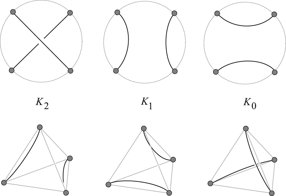
6.3 Cubes of resolutions
The above skein sequence can be seen as a consequence of the fact that the chain complex  $C^{\sharp }_{2}$ that computes
 $I^{\sharp }(K_{2}; \Gamma _{\sigma })$ is quasi-isomorphic to the mapping cone of a chain map
 $C^{\sharp }_{1}\to C^{\sharp }_{0}$. As in [Reference Kronheimer and MrowkaKM12], the skein sequence generalizes as follows. Suppose that
 $Y^{o}$ contains
 $N$ disjoint balls
 $B_{1}$, …,
 $B_{N}$. For each
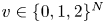 $v\in \{0,1,2\}^{N}$, let there be given a web
 $K_{v}\subset Y^{o}$. Outside the balls, all the
 $K_{v}$ are the same. Inside the ball
 $B_{i}$, the web
 $K_{v}$ coincides with one of the models in Figure 4, according to the value of the coordinate
 $v_{i}$. We write
 $(C^{\sharp }_{v}, d_{v})$ for the standard chain complex that computes
 $I^{\sharp }(K_{v} ; \Gamma _{\sigma })$. (A choice of metric and perturbation is involved.)
Among the  $K_{v}$, we pick out as distinguished the web
 $K_{\mathbf {2}}$, where
 \[ \mathbf{2} = (2,2,\ldots, 2). \]
We also introduce the ‘cube’
 \[ \mathbf{C}^{\sharp} = \bigoplus_{v\in \{0,1\}^{N}} C^{\sharp}_{v}. \]
For each  $v > u$ in
 $\{0,1\}^{N}$, there is a standard cobordism
 $S_{vu}$ from
 $K_{v}$ to
 $K_{u}$, obtained by adding
 $1$-handles in each of the balls
 $B_{i}$ where the coordinates of
 $v$ and
 $u$ differ. If there are
 $n$ such coordinates, then
 $S_{vu}$ carries a standard family
 $G_{vu}$ of metrics, of dimension
 $n-1$, as described in [Reference Kronheimer and MrowkaKM12], which give rise to
 $\mathcal {S}$-module homomorphisms
 \[ f_{vu} : C^{\sharp}_{v} \to C^{\sharp}_{u}. \]
As a special case, we also define  $f_{vv}=d_{v}$. We then define
 \[ \mathbf{F} : \mathbf{C}^{\sharp} \to \mathbf{C}^{\sharp} \]
as
 \[ \mathbf{F} = \bigoplus_{v\ge u}\, f_{vu}. \]
Theorem 6.1 (Theorem 6.8 of [Reference Kronheimer and MrowkaKM12])
The square of  $\mathbf {F}$ is zero, so
 $(\mathbf {C}^{\sharp }, \mathbf {F})$ is a complex of
 $\mathcal {S}$-modules. Furthermore, there is a chain map
 \[ \big(C^{\sharp}_{\mathbf{2}}, d_{\mathbf{2}}\big) \to (\mathbf{C}^{\sharp}, \mathbf{F}) \]
inducing an isomorphism in homology. In particular, the homology of the ‘cube’ complex  $(\mathbf {C}^{\sharp }, \mathbf {F})$ is isomorphic to
 $I^{\sharp }(K_{\mathbf {2}} ; \Gamma _{\sigma })$.
As is standard in Khovanov homology, the cube  $\mathbf {C}^{\sharp }$ has a filtration (increasing, with our conventions),
 \[ \mathcal{F}_{n} \mathbf{C}^{\sharp} = \bigoplus_{ \substack{v\in\{0,1\}^{N} \\ |v| \le n}} C^{\sharp}_{v}. \]
There is a corresponding spectral sequence, just as in [Reference Kronheimer and MrowkaKM12, Corollary 8.1].
Corollary 6.2 For webs  $K_{v}$ as above, there is a spectral sequence of
 $\mathcal {S}$-modules whose
 $E_{1}$ term is
 \[ \bigoplus_{v \in \{0,1\}^{N}} I^{\sharp}(K_{v} ;\Gamma_{\sigma}) \]
and which abuts to the instanton Floer homology  $I^{\sharp }(K_{v} ; \Gamma _{\sigma })$ for
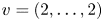 $v=(2,\ldots ,2)$. The differential
 $d_{1}$ is the sum of the maps induced by the cobordisms
 $S_{vu}$ with
 $v>u$ and
 $|v-u|=1$.
6.4 Pants and the $E_{2}$ page

The spectral sequence in Corollary 6.2 is set up quite generally for webs in a fixed 3-manifold, differing by skein moves inside fixed balls. The standard application for this setup is to consider a plane projection and have the fixed balls correspond to the crossings in the projection.
So, let  $K$ be a link in
 $\mathbb{R}^{3}\subset S^{3}$ with a planar projection giving a diagram
 $D$ in
 $\mathbb{R}^{2}$. Let
 $N$ be the number of crossings in the diagram. As in [Reference KhovanovKho00], we can consider the
 $2^{N}$ possible smoothings of
 $D$, indexed by the points
 $v$ of the cube
 $\{0,1\}^{N}$. The conventions we use for the labels
 $\{0,1\}$ is the same as the convention in [Reference KhovanovKho00, Reference RasmussenRas10] and is also consistent with the convention illustrated in Figure 4. The smoothings give
 $2^{N}$ different unlinks
 $K_{v}$ in the plane of the projection. For each
 $v\ge u$ in
 $\{0,1\}^{N}$, we have our standard cobordism
 $S_{vu}$ from
 $K_{v}$ to
 $K_{u}$, with its family of metrics.
We apply Corollary 6.2 to this situation. We learn that there is a spectral sequence abutting to  $I^{\sharp }(K ; \Gamma _{\sigma })$ whose
 $E_{1}$ term is
 \[ E_{1}= \bigoplus_{v\in \{0,1\}^{N}} I^{\sharp}(K_{v} ; \Gamma_{\sigma}) \]
and whose differential  $d_{1}$ is
 \begin{equation} d_{1} = \sum_{|v-u|=1} I^{\sharp}(S_{vu} ; \Gamma_{\sigma}). \end{equation}
In this situation, unlike the general case considered previously, each cobordism  $S_{vu}$ with
 $|v-u|=1$ is a cobordism between planar unlinks, obtained from a ‘pair of pants’ that either joins two components into one, or splits one component into two. Because the unlinks are planar, and the cobordisms
 $S_{vu}$ can be naturally embedded in
 $\mathbb{R}^{3}$, we can consistently orient all the
 $K_{v}$ so that the cobordisms between them are also oriented cobordisms. We have already computed
 $I^{\sharp }(U_{n};\Gamma _{\sigma })$ for an oriented planar unlink
 $U_{n}$ (Corollary 5.7) as well as the maps that arise from the oriented pants and copants cobordisms (§ 5.4). So, we completely understand the
 $E_{1}$ page and its differential
 $d_{1}$. We have
 \[ E_{1}= \bigoplus_{v\in \{0,1\}^{N}} V^{{\otimes} n(v)}, \]
where  $V$ is a free
 $\mathcal {S}$-module of rank
 $2$, admitting a standard basis
 $\mathbf {x}_{+}$,
 $\mathbf {x}_{-}$, and
 $n(v)$ indexes the components of the unlink
 $K_{v}$. Whenever
 $v> u$ and
 $|v-u|=1$, the corresponding summand of
 $d_{1}$ in (50) involves only the factors
 $V$ of the tensor product that are adjacent to the vertex at which
 $v$ and
 $u$ differ, where it is given by
 \begin{equation} I^{\sharp}(\mathord{\Pi}; \Gamma_{\sigma}) : V\otimes V\to V \end{equation}
or
 \begin{equation} I^{\sharp}(\mathord{\amalg}; \Gamma_{\sigma}) :V \to V\otimes V \end{equation}
depending on whether two components of  $K_{v}$ merge in
 $K_{u}$, or one component splits.
In the language of [Reference KhovanovKho06], the  $\mathcal {S}$-module
 $V$ equipped with the multiplication
 $I^{\sharp }(\mathord {\Pi }; \Gamma _{\sigma })$ and comultiplication
 $I^{\sharp }(\mathord {\amalg }; \Gamma _{\sigma })$ is a self-dual, rank-2 Frobenius system
 $\mathcal {F}_{\sigma }$. As an algebra, its unit element is
 $\mathbf {x}_{+}$, and its co-unit is
 $\mathbf {y}_{+}$ (Definition 5.3). The multiplication is described completely by giving the square of the element
 $x=\mathbf {x}_{-}$, the formula for which is in (44). So, we can write it as
 \[ \mathcal{S}[x] \big/ \big( x^{2} + \sigma(P) x + \sigma(Q) \big). \]
Our description of  $(E_{1}, d_{1})$ above coincides with Khovanov's definition of the complex that computes the knot homology group corresponding to this Frobenius system. There is only the slight change of conventions, because of the historically reversed roles of the two smoothings
 $\{0,1\}$. With that understood, we can identify the
 $E_{2}$ page of the spectral sequence.
Proposition 6.3 In the special case that the cube of resolutions is the one obtained from a planar diagram of a knot or link  $K$, the
 $E_{2}$ page of the spectral sequence in Corollary 6.2 is isomorphic to the knot homology
 $H(\bar {K}; \mathcal {F}_{\sigma })$ in the notation of [Reference KhovanovKho06], where
 $\mathcal {F}_{\sigma }$ is the rank-2 Frobenius system over
 $\mathcal {S}$ given by the multiplication (51) and comultiplication (52). Here
 $\bar {K}$ denotes the mirror image of
 $K$.
Corollary 6.4 For a knot or link  $K$ in
 $\mathbb{R}^{3}$, there is a spectral sequence whose
 $E_{2}$ page is Khovanov's homology
 $H(\bar {K}; \mathcal {F}_{\sigma })$ corresponding to the Frobenius system
 $\mathcal {F}_{\sigma }$ and which abuts to the instanton homology with local coefficients,
 $I^{\sharp }(K; \Gamma _{\sigma })$.
Theorem 1.1 in the introduction, along with its two corollaries, are obtained directly from Corollary 6.4 by identifying the Frobenius system  $\mathcal {F}_{\sigma }$ in each case, to compare it with those described in the notation of [Reference KhovanovKho06]. We begin with the case that
 $\mathcal {S}=\mathcal {R}$ and
 $\sigma =1$ (i.e. the case of the local system
 $\Gamma$). Here the resulting Frobenius system
 $\mathcal {F}$ corresponds to
 \[ \mathcal{R}[x] \big/ \big( x^{2} + P x + Q \big). \]
As explained in the introduction, the universal example from [Reference KhovanovKho06], when reduced mod  $2$, is a Frobenius system
 $F_{5}$ over
 \[ R_{5} = \mathbb{F}_{2}[h,t]. \]
Its multiplication is given by
 \[ R_{5}[x] / ( x^{2} + h x + t ). \]
Since the comultiplications can be compared similarly, we see that the Frobenius system  $\mathcal {F}$ arising from
 $I^{\sharp }$ with coefficient system
 $\Gamma$ is
 $F_{5}\otimes _{r} \mathcal {R}$, where
 $r$ maps
 $h$ to
 $P$ and
 $t$ to
 $Q$. Theorem 1.1 is therefore a consequence of Corollary 6.4.
Corollaries 1.2 and 1.3 follow from this universal version by base change, as explained in the introduction.
6.5 The spectral sequence for reduced homologies
There is also a version of Corollaries 1.2 and 1.3 for the reduced homology theories. Given a link with a base point, and given a diagram for the link such that the base point does not lie at a crossing, we may form again the cube of resolutions and, for each vertex of the cube, we now have a planar unlink with a single marked point. Let  $\sigma :\mathcal {R}\to \mathcal {S}$ be a base change with
 $\sigma (T_{0}) = \sigma (T_{1})$, so that the reduced theory
 $I^{\natural }$ is defined. The basic spectral sequence described in Corollary 6.2 has a reduced counterpart, whose statement and proof are essentially the same.
Proposition 6.5 There is a spectral sequence of  $\mathcal {S}$-modules whose
 $E_{1}$ term is
 \[ \bigoplus_{v \in \{0,1\}^{N}} I^{\natural}(K_{v} ;\Gamma_{\sigma}) \]
and which abuts to the instanton Floer homology  $I^{\sharp }(K_{v} ; \Gamma _{\sigma })$ for
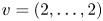 $v=(2,\ldots ,2)$. The differential
 $d_{1}$ is the sum of the maps induced by the cobordisms
 $S_{vu}$ with
 $v>u$ and
 $|v-u|=1$.
The condition that  $\sigma (T_{0})=\sigma (T_{1})$ implies that the Frobenius system
 $\mathcal {F}_{\sigma }$ has a description in which the algebra is
 \[ \mathcal{S}[M] / (M^{2} + \sigma(P) M) \]
and the comultiplication is given by
 \begin{align*} 1&\mapsto 1\otimes M + M\otimes 1 + \sigma(P)(1\otimes 1), \\ M& \mapsto M\otimes M. \end{align*}
In such a situation, there is a reduced link homology  $\tilde {H} (\bar {K} ; \mathcal {F}_{s})$ obtained from the cube of resolutions. It is defined from a complex
 $\tilde {C}$ for which the contribution
 $\tilde {C}_{v}$ from a vertex of the cube is
 \[ \tilde{\mathcal{A}} \otimes_{\mathcal{S}} \mathcal{A} \otimes_{\mathcal{S}} \cdots \otimes_{\mathcal{S}} \mathcal{A}, \]
where  $\mathcal {A}$ is the Frobenius algebra of
 $\mathcal {F}_{\sigma }$ and
 $\tilde {\mathcal {A}}$ is the
 $\mathcal {S}$-submodule generated by
 $m$. The tensor product is over all components of the unlink
 $K_{v}$ and the factor
 $\tilde {\mathcal {A}}$ corresponds to the component with the base point. The edge maps as usual come from the multiplication and comultiplication, restricted to
 $\tilde {\mathcal {A}} \subset \mathcal {A}$ if necessary.
Using Proposition 5.10 and Corollary 5.11 for the edges involving the component with the base point, we can match up the differential  $d_{1}$ in Proposition 6.5 with the multiplication and comultiplication maps of
 $\tilde {\mathcal {A}}\otimes \mathcal {A} \to \tilde {\mathcal {A}}$ and
 $\tilde {\mathcal {A}} \to \tilde {\mathcal {A}} \otimes \mathcal {A}$.
We obtain in this way a reduced counterpart to Corollary 1.2.
Corollary 6.6 There is a spectral sequence of modules over the Laurent series ring  $\mathcal {S}_{\mathop {\mathsf {BN}}\nolimits }$ in three variables, from the reduced version of graded Bar-Natan homology in characteristic
 $2$,
 \[ \widetilde{\mathop{\mathsf{BN}}\nolimits}(\bar{K}) \otimes_{r_{1}} \mathcal{S}_{\mathop{\mathsf{BN}}\nolimits} \implies I^{\natural}(K ; \Gamma_{\mathop{\mathsf{BN}}\nolimits}), \]
to the reduced instanton homology group with coefficients in the local system  $\Gamma _{\mathop {\mathsf {BN}}\nolimits }= \Gamma \otimes _{\sigma _{{bn}}}\mathcal {S}_{\mathop {\mathsf {BN}}\nolimits }$, where the base change
 $\sigma _{bn}$ is given by (10).
The reduced version of Corollary 1.3, for filtered Bar-Natan homology, can be formulated in the same way.
Corollary 6.7 For a knot or link  $K$, let
 $\widetilde {\mathop {\mathsf {fBN}}\nolimits }(K)$ denote the reduced version of filtered Bar-Natan homology over
 $\mathbb{F}_{2}$. Then there is a spectral sequence of vector spaces over
 $\mathbb{F}_{4}$,
 \[ \widetilde{\mathop{\mathsf{fBN}}\nolimits}(\bar{K})\otimes \mathbb{F}_{4} \implies I^{\natural}(K ; \Gamma_{\mathop{\mathsf{fBN}}\nolimits}), \]
where  $\Gamma _{\mathop {\mathsf {fBN}}\nolimits }$ is the local system of
 $\kern0.05em \mathbb{F}_{4}$ vector spaces obtained from
 $\Gamma$ by the base change (12).