


1 Introduction
Since the discovery of pulsars in 1967 (Hewish et al. Reference Hewish, Bell, Pilkington, Scott and Collins1968), and the realization of the basic nature of pulsar-wind nebulae shortly thereafter, pulsars and PWNe have served as fertile fields for the study of relativistic flows and particle acceleration. The problems posed by these objects include the mechanism of generating a relativistic outflow; the nature of that outflow and even its composition; the distribution of energy between particles and magnetic field and the energy distribution among the particles; the nature of highly relativistic shock waves; and many others. PWNe exhibit a broadband spectrum which may range over 20 orders of magnitude in photon energy from radio to TeV gamma rays, whose interpretation casts light on the nature of particle energization in the pulsar–PWN system.
A defining characteristic of PWNe from the original recognition of the class (Weiler & Panagia Reference Weiler and Panagia1978) has been a flat radio spectrum (energy index
 $\unicode[STIX]{x1D6FC}_{r}\sim -0.4{-}0$
, where
 $S_{\unicode[STIX]{x1D708}}\propto \unicode[STIX]{x1D708}^{\unicode[STIX]{x1D6FC}}$
, so
 $\unicode[STIX]{x1D6FC}=1-\unicode[STIX]{x1D6E4}$
,
 $\unicode[STIX]{x1D6E4}$
the photon index). Some spectra were so flat that they could have been mistaken for optically thin thermal bremsstrahlung (
 $\unicode[STIX]{x1D6FC}_{r}=-0.1$
), were it not for the detection of strong polarization, another defining characteristic of the class, and confirming the synchrotron interpretation – although indicating a population of relativistic leptons with a far harder energy distribution
 $N(E)\propto E^{-s}$
, with
 $s\sim 1{-}1.8$
, than seen in most other synchrotron sources such as radio galaxies or shell supernova remnants (SNRs), where
 $s\sim 2{-}3$
. That synchrotron spectrum is observed in a few cases to extend from low radio frequencies where interstellar free–free absorption cuts it off, all the way to the highest photon energies producible by synchrotron emission: in the absence of special conditions, of order
 ${\sim}30$
MeV (e.g. de Jager et al.
Reference de Jager, Harding, Michelson, Nel, Nolan, Sreekumar and Thompson1996).
Gamma-ray emission from the Crab Nebula was originally predicted by Gould (Reference Gould1965) as inverse-Compton upscattering of the primary synchrotron spectrum of radio through X-rays. Virtually all models since that time (notably, de Jager & Harding Reference de Jager and Harding1992) have recognized that inverse-Compton (IC) emission is unavoidable and probably responsible for any emission detectable above a few hundred MeV, although the seed-photon sources may vary: IC from the source’s own synchrotron photons is known as synchrotron self-Compton (SSC), and scattering from cosmic microwave background (CMB) photons is known as ICCMB. It is also possible that local infrared (IR) fields provide the dominant photon energy density from which to produce GeV to TeV photons. However, in a few cases (e.g. Li, Chen & Zhang Reference Li, Chen and Zhang2010), hadronic contributions to GeV–TeV emission (decay of
 $\unicode[STIX]{x03C0}^{0}$
mesons created in inelastic collisions between relativistic protons and thermal gas) may be important.
A critical question in high-energy astrophysics in most of its manifestations involves the maximum energies to which non-thermal particles can be accelerated. This is an important issue for the interpretation of quasar spectra, of supernova remnants and PWNe, of cosmic rays and of cosmic neutrino observations. The best observational constraints on the acceleration processes can be found in well-characterized sources, spatially resolved if possible, for which various important parameters such as shock speeds, densities and magnetic-field strengths can be determined independently. One of the best motivations for the detailed study of PWN emission at all energies is the hope of obtaining generally applicable insights into the particle acceleration process.
The synchrotron/IC interpretation of the broadband spectral energy distribution (SED) of PWNe gives us two opportunities to study the electron distribution at the highest energies. The synchrotron component turns over (in
 $E^{2}F_{E}$
space) in the X-ray regime, showing the steepening spectrum as it cuts off. Those electrons upscatter whatever photons are available, so (modulo Klein–Nishina effects) the resulting GeV/TeV emission also reflects the cutoff in the electron spectrum. Comparing the two not only gives a clearer picture of the shape of the spectrum, but may allow the inference of the magnetic-field strength.
However, these effects can be blurred by spatial inhomogeneities. Until recently, the hard X-ray part of the spectrum was inaccessible or poorly known for all PWNe except the Crab, and even there, imaging was not available. The launch of the NuSTAR mission in 2012 made available, for the first time, true imaging in the energy range above 10 keV, allowing detailed investigation of the synchrotron spectrum and, at the
 ${\sim}1^{\prime }$
level, the spatial structure, of several bright PWNe. The results provide additional insight into the behaviour of the electron spectrum in the 10–100 TeV range, and constrain the interpretation of the GeV/TeV emission seen from these objects.
2 Observations
The NuSTAR mission (Harrison et al.
Reference Harrison, Craig, Christensen, Hailey, Zhang, Boggs, Stern, Cook, Forster and Giommi2013) has opened the hard X-ray sky to true imaging since July 2012. The two independent telescopes and charge-coupled device (CCD) detectors (focal plane mirror assemblies A and B, or FPMA and FPMB) provide spectral coverage between 3 and 79 keV. The angular resolution (50 % enclosed energy diameter) is approximately
 $1^{\prime }$
. (However, the full width at half maximum (FWHM) is only
 ${\sim}18^{\prime \prime }$
, roughly independent of energy above 10 keV.) The time resolution is
 $2~\unicode[STIX]{x03BC}\text{s}$
. The spectral coverage below 10 keV overlaps with that of Chandra and XMM-Newton, whose much higher angular resolution complements the higher-energy response of NuSTAR.
Observations of PWNe with NuSTAR are ongoing. Here I will summarize results on three prominent PWNe: the Crab Nebula, G21.5–0.9 and MSH 15–52. Table 1 lists the basic observational properties. More details on each can be found in primary publications referenced in the table. All three objects contain radio pulsars and have been detected at TeV wavelengths, as described below. For the Crab and MSH 15–52, the pulsar contributes a significant fraction of the flux in the NuSTAR band, so phase-resolved spectroscopy is necessary to recover the spectrum of the nebula, as the pulsar spectrum is quite distinct. G21.5–0.9 contains a 62 ms radio pulsar with a very high energy-loss rate (
 ${\dot{E}}=3.3\times 10^{37}~\text{erg}~\text{s}^{-1}$
; Gupta et al.
Reference Gupta, Mitra, Green and Acharyya2005; Camilo et al.
Reference Camilo, Ransom, Gaensler, Slane, Lorimer, Reynolds, Manchester and Murray2006). A central compact X-ray source, presumably the pulsar, has less than 3 % of the flux between 2 and 8 keV of the entire nebula (Matheson & Safi-Harb Reference Matheson and Safi-Harb2010), and is not observed to pulse in X-rays.
Throughout this paper, all quoted NuSTAR errors are 90 % confidence intervals.
Summary of NuSTAR PWN observations.

2.1 Crab Nebula
The Crab Nebula, in spite of its iconic status, continues to surprise. Its brightness at soft X-ray wavelengths, and apparent simplicity of spectrum, well described by a power law with photon index
 $\unicode[STIX]{x1D6E4}=2.1\pm 0.03$
(Kirsch et al.
Reference Kirsch, Schönherr, Kendziorra, Freyberg, Martin, Wilms, Mukerjee, Breitfellner, Smith and Staubert2006), have led to its status as a primary calibrator for X-ray instruments. However, efforts to confirm, rather than simply assume, its stability have led to discoveries of variations on year time scales. Wilson-Hodge et al. (Reference Wilson-Hodge, Cherry, Case, Baumgartner, Beklen, Narayana Bhat, Briggs, Camero-Arranz, Chaplin and Connaughton2011) conducted an exhaustive cross-comparison study of various hard X-ray missions, and found flux variations of 3–4 %
 $\text{yr}^{-1}$
, with a systematic decrease of 7 % between 2008 and 2010. More spectacularly, gamma-ray flares have been observed, with remarkable properties posing significant challenges to theorists. See Bühler & Blandford (Reference Bühler and Blandford2014) for a review.
The Crab is a relatively small source (about
 $5^{\prime }\times 7^{\prime }$
) compared to angular resolutions of instruments sensitive above 10 keV. For many years, the only information on the Crab’s morphology above that energy came from lunar occultation measurements made with a sounding rocket (Kestenbaum et al.
Reference Kestenbaum, Ku, Novick and Wolff1975; Ku et al.
Reference Ku, Kestenbaum, Novick and Wolff1976), which were fit with a Gaussian in several energy ranges, to obtain a dependence of FWHM with energy of (FWHM)
 $\propto E^{m}$
with
 $m=-0.148\pm 0.012$
. This rate of shrinkage is quite consistent with the prediction of
 $m=-1/9$
based on energy-loss-limited advection in a spherical magnetohydrodynamic (MHD) flow (Kennel & Coroniti Reference Kennel and Coroniti1984a
,Reference Kennel and Coroniti
b
; KC84).
NuSTAR observed the Crab as a calibrator 16 times between 2012 September 20 and 2013 November 11, mostly for observations of 2–5 ks (Madsen et al. Reference Madsen, Harrison, Markwardt, An, Grefenstette, Bachetti, Miyasaka, Kitaguchi, Bhalerao and Boggs2015a ). The high time resolution allowed the division of these data into 13 equal phase bins across the pulse period of 33 ms. Significant pulsed emission can be seen in all but three bins (10–12), so nebular spectral analysis was confined to those. The full analysis of these observations is contained in Madsen et al. (Reference Madsen, Reynolds, Harrison, An, Boggs, Christensen, Craig, Fryer, Grefenstette and Hailey2015b ); here I provide a summary.
Crab images, after maximum-likelihood deconvolution (Madsen et al. Reference Madsen, Reynolds, Harrison, An, Boggs, Christensen, Craig, Fryer, Grefenstette and Hailey2015b , figure 11). Note more rapid shrinkage of the northwest counter-jet, and narrowing of the torus.

(a) Contours of the half-width at half maximum (HWHM) for various energy bands (Madsen et al. Reference Madsen, Reynolds, Harrison, An, Boggs, Christensen, Craig, Fryer, Grefenstette and Hailey2015b , figure 12). From the outside in, 3–5, 5–6, 6–8, 8–12, 12–20, 20–35 and 35–78 keV. (b) HWHM in arcseconds, measured from the pulsar location along the torus and jet axis in the directions (a–b) northeast (NE), southwest (SW), northwest (NW), southeast (SE) (Madsen et al. Reference Madsen, Reynolds, Harrison, An, Boggs, Christensen, Craig, Fryer, Grefenstette and Hailey2015b , figure 14). The torus extends along the NE–SW axis. The NW counter-jet shrinks at a rate considerably faster than the other three directions.

2.1.1 Spatial analysis
A subset of the observations, those with off-axis angles less than
 $2^{\prime }$
and well away from detector gaps, was selected for imaging analysis. The small spatial variations in the point-spread function (PSF) are minimized for this subset. Again, only phase bins 10–12 were used to minimize pulsar contamination. Vignetting corrections were applied, appropriate to each of the energy bins shown in figure 1.
Clear morphological trends with energy are apparent in figure 1. The central torus oriented NE–SW shows only slight shrinkage along the (projected) major axis as energy increases, but the ‘counter-jet’ that extends to the NW shrinks much more markedly. The shrinkage rates are illustrated in figure 2 (Madsen et al.
Reference Madsen, Reynolds, Harrison, An, Boggs, Christensen, Craig, Fryer, Grefenstette and Hailey2015b
). The power-law fits to those extents (
 $\text{HWHM}\propto E^{m}$
) give
 $m=-0.086\pm 0.025$
,
 $-0.073\pm 0.028$
, and
 $-0.218\pm 0.040$
for the NE, SW and NW directions respectively. (The SE measurements are consistent with zero.) The torus rates are slightly smaller than the prediction of the MHD model of Kennel & Coroniti (Reference Kennel and Coroniti1984a
) (
 $m=-1/9$
) and the earlier measurements summarized in Ku et al. (Reference Ku, Kestenbaum, Novick and Wolff1976) of
 $m=-0.148\pm 0.012$
. However, the NW ‘counter-jet’ clearly shrinks much more rapidly. In the standard interpretation, this size shrinkage, coupled with spectral steepening, is due to ‘synchrotron burnoff’, the loss of higher-energy electrons due to synchrotron losses, whose rate is proportional to the square of the electron energy. In a homogeneous source, the electron energy distribution will steepen by one power above an energy at which the source lifetime equals the radiative lifetime (Kardashev Reference Kardashev1962), and the synchrotron spectrum will steepen by 0.5. That is, for an injected
 $E^{-s}$
spectrum of electron energies,
 $s\rightarrow s+1$
, and for the emitted photon power law
 $(h\unicode[STIX]{x1D708})^{-\unicode[STIX]{x1D6E4}}$
,
 $\unicode[STIX]{x1D6E4}$
steepens to
 $\unicode[STIX]{x1D6E4}+0.5$
above that energy. However, if source gradients are present, the steepening may be larger or smaller (see below). In the KC84 spherical model, which does not attempt to address the radio portion of the Crab’s spectrum, the injected electron spectrum
 $N(E)=KE^{-2.2}$
accounts for the optical emission, steepening somewhere in the ultraviolet (UV) so that at X-ray energies, electrons are not able to advect as far as the edge of the remnant. This shrinking of the effective source size gives rise to the steeper spectrum. However, our results show the highly anisotropic nature of the shrinkage, so that a more sophisticated model is clearly required.
Crab Nebula spectrum within
 $13^{\prime \prime }$
of the pulsar, for off-source bins 10–12 (Madsen et al.
Reference Madsen, Reynolds, Harrison, An, Boggs, Christensen, Craig, Fryer, Grefenstette and Hailey2015b
, figure 6). The black and red data are the same, but divided by different models. The red curve shows the best-fit broken power law, with
 $\unicode[STIX]{x1D6E4}_{1}=1.91\pm 0.01$
to a break energy
 $E_{b}=8.7\pm 0.9$
keV and above that
 $\unicode[STIX]{x1D6E4}_{2}=2.03\pm 0.01$
. The black curve has
 $\unicode[STIX]{x1D6E4}=\unicode[STIX]{x1D6E4}_{2}$
at all energies, and is scaled to be the same at high energies.

Break energy
 $E_{b}$
(a,b) and change in photon index
 $\unicode[STIX]{x0394}\unicode[STIX]{x1D6E4}\equiv \unicode[STIX]{x1D6E4}_{2}-\unicode[STIX]{x1D6E4}_{1}$
(c,d) for the Crab Nebula (Madsen et al.
Reference Madsen, Reynolds, Harrison, An, Boggs, Christensen, Craig, Fryer, Grefenstette and Hailey2015b
, figure 7). Colours are NuSTAR data, and are the same in the two columns; the left two images show NuSTAR intensity contours, while the right two show Chandra contours. The cross on the left indicates the pulsar position. The pixels represent central values of boxes
 $24.5^{\prime \prime }$
on a side slid across the nebula in increments of
 $2.45^{\prime \prime }$
, a NuSTAR pixel, so they are highly correlated.

2.1.2 Spectral analysis
While the spatially and phase-integrated spectrum of the Crab Nebula plus pulsar has been calibrated to the standard
 $\unicode[STIX]{x1D6E4}=2.1$
power law, our results show that closer to the pulsar (within an extraction radius of
 $50^{\prime \prime }$
), a simple power law is not adequate to describe the data for the nebular (off-pulse; phase bins 10–12) spectrum. Instead, we require steepening in the NuSTAR range between 3 and 78 keV. The effect is not large; many parameterizations are available to describe a slow steepening. We chose one of the simplest, a broken power law whose three free parameters are the two power-law indices and the ‘break’ energy
 $E_{b}$
where they meet. Figure 3 compares the observed fluxes to a single power law for a subset of the data within approximately
 $13^{\prime \prime }$
of the pulsar, with
 $\unicode[STIX]{x1D6E4}_{1}=1.91\pm 0.01$
,
 $\unicode[STIX]{x1D6E4}_{2}=2.03\pm 0.01$
, and
 $E_{b}=8.7\pm 0.9$
keV.
Figure 4 shows that the required steepening is a strong function of position, with considerably greater steepening to the northwest of the pulsar, consistent with the spatial analysis. However, the
 ${\sim}1^{\prime }$
PSF of NuSTAR mixes regions of different spectral shape, so that figure 4 underestimates the actual breaks. In an attempt to correct for this smoothing, we adopted a spatial model for the Crab based on Chandra data (Mori et al.
Reference Mori, Burrows, Hester, Pavlov, Shibata and Tsunemi2004), dividing the nebula into five different regions as shown in figure 5. We found that, after convolution with NuSTAR’s PSF, a reasonably good match to figure 4 could be obtained with a steepening
 $\unicode[STIX]{x0394}\unicode[STIX]{x1D6E4}$
of approximately 0.25 at 9 keV, integrated over the torus structure. Further work is underway to refine this conclusion, but substantial spectral steepening at small radii is clearly necessary. It is not terribly surprising that this steepening was not obvious previously; first, it would not be apparent for CCD imaging missions like Chandra and XMM-Newton whose response only extends to approximately 10 keV; and second, the harder-spectrum pulsar will contaminate nebular observations that are not restricted to pulse-off phases.
Input model for spectral steepening estimate. The brightness normalizations for the different regions were set in the 2–10 keV range using Chandra observations (Mori et al. Reference Mori, Burrows, Hester, Pavlov, Shibata and Tsunemi2004).

2.2 G21.5–0.9
This object consists of a bright PWN approximately
 $40^{\prime \prime }$
in radius, inside faint diffuse emission with an incomplete shell at a radius of approximately
 $2^{\prime }$
(Safi-Harb et al.
Reference Safi-Harb, Harrus, Petre, Pavlov, Koptsevich and Sanwal2001, see figure 6). The diffuse emission is primarily due to scattering of the bright PWN by intervening dust (Bandiera & Bocchino Reference Bandiera and Bocchino2004), but the brightest knots in the incomplete shell show a thermal spectrum (Bocchino Reference Bocchino2005), with perhaps a non-thermal component. The most straightforward interpretation is that the shell represents the supernova remnant (SNR) blast wave, with the non-thermal component presumably synchrotron emission from shock-accelerated electrons.
At radio frequencies, the PWN has a typical flat spectrum with radio energy index
 $\unicode[STIX]{x1D6FC}_{r}=0.0\pm 0.1$
(Bietenholz et al.
Reference Bietenholz, Matheson, Safi-Harb, Brogan and Bartel2011). The brightest knot in the partial shell (‘North Spur’ in figure 6) is seen at radio wavelengths (Bietenholz et al.
Reference Bietenholz, Matheson, Safi-Harb, Brogan and Bartel2011), but is quite faint. The integrated spectrum begins to steepen above approximately 30 GHz (Salter et al.
Reference Salter, Reynolds, Hogg, Payne and Rhodes1989). G21.5–0.9 has also been detected at TeV wavelengths, by the H.E.S.S. air-Čerenkov telescope (Djannati-Ataï et al.
Reference Djannati-Ataï, deJager, Terrier, Gallant and Hoppe2008).
(a) Chandra image of G21.5–0.9 between 3 and 6 keV (Matheson & Safi-Harb Reference Matheson and Safi-Harb2005). (b)–(f): Deconvolved NuSTAR images in various bands. (b) 3–6 keV; (c) 6–10 keV; (d) 10–15 keV; (e) 15–20 keV; (f) 20–25 keV.

2.2.1 Spectral analysis
Like the Crab, G21.5–0.9 shows progressive steepening in power-law fits to soft X-ray emission at larger radii (Safi-Harb et al.
Reference Safi-Harb, Harrus, Petre, Pavlov, Koptsevich and Sanwal2001). NuSTAR observed G21.5–0.9 on four occasions; the observations are described in detail in Nynka et al. (Reference Nynka, Hailey, Reynolds, An, Baganoff, Boggs, Christensen, Craig, Gotthelf and Grefenstette2014). Our NuSTAR data integrated over the source, show, as for the Crab, a spectral steepening in the vicinity of 10 keV (figure 7). (Interstellar medium (ISM) absorption is low above 3 keV; in the fits we have frozen the column density
 $N_{H}$
to the value
 $2.99\times 10^{22}~\text{cm}^{-2}$
obtained by Tsujimoto et al. (Reference Tsujimoto, Guainazzi, Plucinsky, Beardmore, Ishida, Natalucci, Posson-Brown, Read, Saxton and Shaposhnikov2011) as part of an extensive cross-calibration study using bright compact X-ray sources.) Again, we use a simple parameterization for the steepening, a broken power law, and find
 $\unicode[STIX]{x1D6E4}_{1}=1.996\pm 0.013$
below a break energy
 $E_{b}=9.7_{-1.4}^{+1.2}$
keV, and
 $\unicode[STIX]{x1D6E4}_{2}=2.093\pm 0.013$
above. Effects of dust scattering are expected to be small above 3 keV. While G21.5–0.9 is not much larger than NuSTAR’s PSF, limited spatially resolved spectroscopy was possible, confirming both the progressive spectral steepening with radius, and the requirement for a spectral break. (For radii beyond
 $60^{\prime \prime }$
, a break is not required, but at those radii, the flux is primarily scattered X-rays, heavily contaminated with central PWN emission by the NuSTAR PSF.)
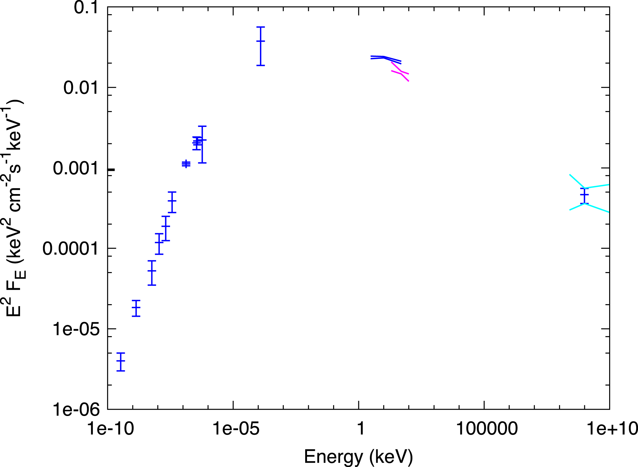
The complete radio–TeV SED is shown in figure 8. The NuSTAR results are marginally inconsistent with those from INTEGRAL (de Rosa et al.
Reference de Rosa, Ubertini, Campana, Bazzano, Dean and Bassani2009), but since G21.5–0.9 is smaller than the INTEGRAL PSF, we regard this difference as insignificant. The H.E.S.S. team (Djannati-Ataï et al.
Reference Djannati-Ataï, deJager, Terrier, Gallant and Hoppe2008) reports a differential photon flux of
 $(4.59\pm 1.00)\times 10^{-13}~\text{cm}^{-2}~\text{s}^{-1}~\text{TeV}^{-1}$
between 0.3 and 40 TeV, with a power-law index of
 $\unicode[STIX]{x1D6E4}=2.08\pm 0.22_{stat}\pm 0.1_{syst}$
. This flux is approximately 2 % of that of the Crab.
NuSTAR spectrum of G21.5–0.9 between 3 and 45 keV (extraction radius
 $165^{\prime \prime }$
) (Nynka et al.
Reference Nynka, Hailey, Reynolds, An, Baganoff, Boggs, Christensen, Craig, Gotthelf and Grefenstette2014, figure 1). Eight spectra (four each from the two mirror assemblies, from the four separate observations) are plotted in different colours, showing the consistency among observations. The requirement of steepening is apparent in (b,c) showing residuals from fits with a single power law (b) and broken power law (c). Neither model is plotted in (a).

G21.5–0.9 spectral energy distribution. Radio-mm points from Salter et al. (Reference Salter, Reynolds, Hogg, Payne and Rhodes1989); IR point from Zajczyk et al. (Reference Zajczyk, Gallant, Slane, Reynolds, Bandiera, Gouiffès, Le Floc’h, Comerón and Koch Miramond2012); blue bowtie, these data (Nynka et al. Reference Nynka, Hailey, Reynolds, An, Baganoff, Boggs, Christensen, Craig, Gotthelf and Grefenstette2014); magenta bowtie, INTEGRAL (de Rosa et al. Reference de Rosa, Ubertini, Campana, Bazzano, Dean and Bassani2009); TeV bowtie in cyan, H.E.S.S. (Djannati-Ataï et al. Reference Djannati-Ataï, deJager, Terrier, Gallant and Hoppe2008).
2.2.2 Spatial analysis
The NuSTAR images of figure 6 show that the structures beyond the central PWN are detected up to at least 20 keV, supporting (but not demanding) the presence of a non-thermal component in the shell emission. Even if the emission is thermal, the required temperature would be substantial, consistent with the identification of these structures with the SNR blast wave (Nynka et al.
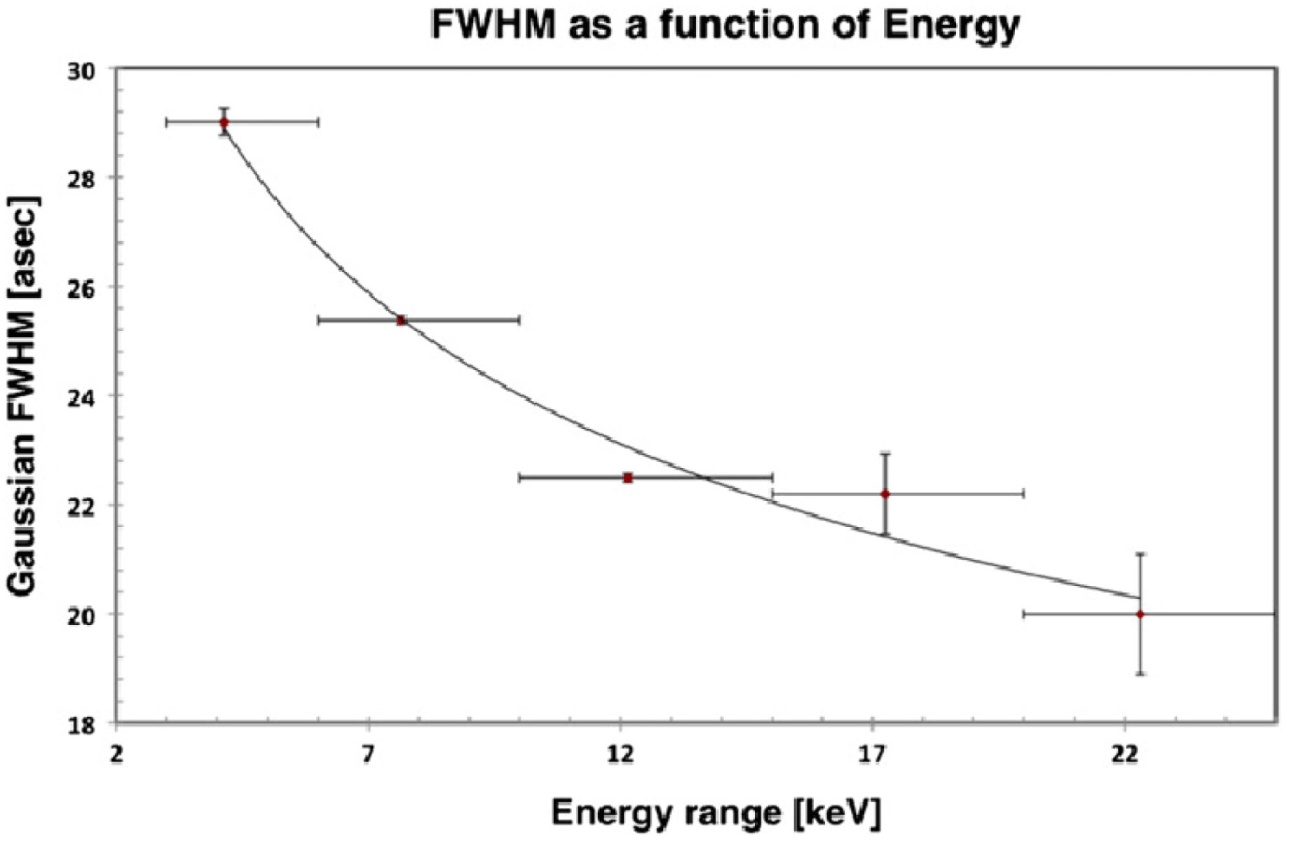
Reference Nynka, Hailey, Reynolds, An, Baganoff, Boggs, Christensen, Craig, Gotthelf and Grefenstette2014). The shrinkage of the PWN is apparent (though overemphasized by the use of a fixed brightness scale), and as for the Crab, can be characterized by a power law in energy, FWHM
 $\propto E^{m}$
with
 $m=-0.21\pm 0.01$
(figure 9).
Two- dimensional Gaussian fit to FWHM of G21.5–0.9 (Nynka et al.
Reference Nynka, Hailey, Reynolds, An, Baganoff, Boggs, Christensen, Craig, Gotthelf and Grefenstette2014, figure 4). The FWHM values shown were measured for the indicated energy bins, with the flux-weighted mean energy for each bin indicated as the data point. The fit gives FWHM
 $\propto E^{m}$
with
 $m=-0.21\pm 0.01$
.
The value of
 $m$
is the same as that determined for the Crab’s NW emission, but substantially larger than for the Crab’s torus diameter (NE–SW). This issue will be discussed below.
2.3 MSH 15–52
By far the most morphologically complex of the three PWNe observed by NuSTAR in its first two years of operation is the peculiar object known commonly by its radio designation MSH 15–52 (or G320.4–1.2) (figure 10). It contains a well-studied pulsar, PSR 1509-58, with a 150-ms period and 1600-year spindown time scale
 $P/2{\dot{P}}$
(Seward & Harnden Reference Seward and Harnden1982), suggesting that MSH 15–52 is quite a young object in spite of its complex appearance. In soft X-rays, a broad somewhat curved structure often called the ‘jet’ extends to the SE. Fainter X-ray emission also extends to the north, eventually meeting an optical nebulosity catalogued as RCW 89. The radio counterpart of MSH 15–52 (Gaensler et al.
Reference Gaensler, Brazier, Manchester, Johnston and Green1999) is faint and poorly correlated with the structure seen by Chandra (Gaensler et al.
Reference Gaensler, Arons, Kaspi, Pivovaroff, Kawai and Tamura2002, figure 11).
The marked absence of an obvious radio PWN is a property MSH 15–52 shares with many PWNe discovered in TeV emission. Figure 11 shows a large field containing all the structure seen in X-rays. The pulsar location is indicated; there is no resemblance between figures 10 and 11. A more violent stretch of the transfer function (figure 11b) shows that if anything, there is an anticorrelation between faint radio and X-ray emission. For modelling purposes, an estimate of radio flux that could be attributed to MSH 15–52 is necessary; Gaensler et al. (Reference Gaensler, Arons, Kaspi, Pivovaroff, Kawai and Tamura2002) make a rough estimate of
 $4\pm 2$
Jy at both 843 and 1400 MHz.
Like the other two targets, MSH 15–52 has also been detected at TeV wavelengths by Aharonian et al. (Reference Aharonian, Akhperjanian, Aye, Bazer-Bachi, Beilicke, Benbow, Berge, Berghaus, Bernlöhr and Boisson2005), who fit observations between 0.3 and 40 TeV with a power-law model. They obtain a differential photon flux of
 $5.7\pm 0.2~\text{(stat)}\pm 1.4~\text{(syst)}\times 10^{-12}~\text{photons}~\text{cm}^{-2}~\text{s}^{-1}~\text{TeV}^{-1}$
, with a photon index of
 $\unicode[STIX]{x1D6E4}=2.27\pm 0.03~\text{(stat)}\pm 0.20~\text{(syst)}$
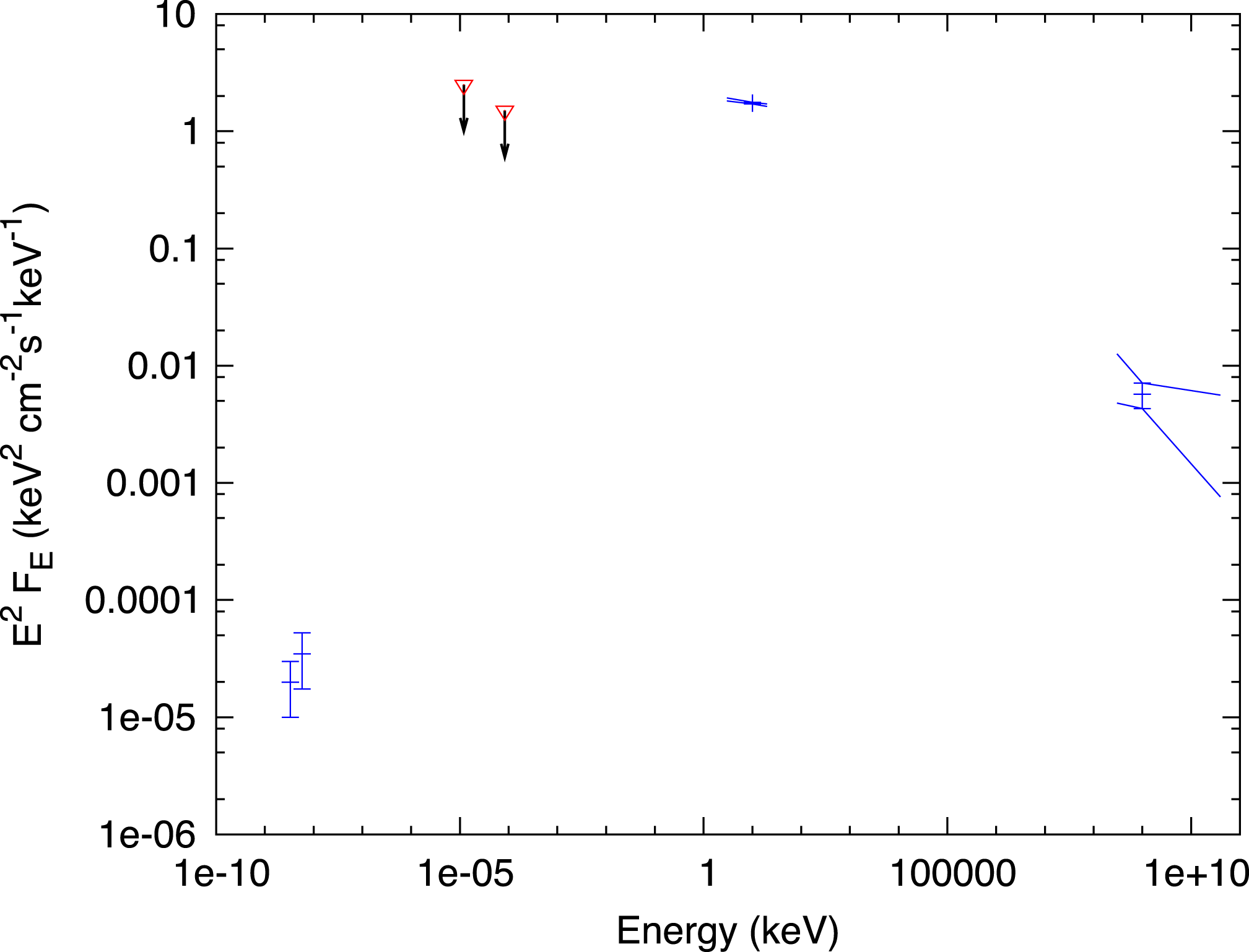
. The full (somewhat sparse) SED of MSH 15–52 is shown in figure 12.
NuSTAR and Chandra images of MSH 15–52 in a
 $10^{\prime }\times 12^{\prime }$
region (An et al.
Reference An, Madsen, Reynolds, Kaspi, Harrison, Boggs, Christensen, Craig, Fryer and Grefenstette2014, figure 2). (a) Combined NuSTAR and Chandra data between 0.5 and 40 keV. (b) Chandra 0.5–2 keV; (c) Chandra 2–4 keV; (d) Chandra 4–7 keV; (e) NuSTAR 3–7 keV; (f) NuSTAR 7–12 keV; (g) NuSTAR 12–25 keV; (h) NuSTAR 25–40 keV; (i) NuSTAR exposure map, with image frame shown. A
 $30^{\prime \prime }$
circle is shown for reference. Colour scales are logarithmic; background levels differ.

Radio images of MSH 15–52. (a) 1344 MHz image made with ATCA (Gaensler et al. Reference Gaensler, Brazier, Manchester, Johnston and Green1999). The brightest structure is the H II region RCW 89, at the top left in figure 10. The pulsar location is marked with a cross. (b) Deeper version of the ATCA radio image (Gaensler et al. Reference Gaensler, Arons, Kaspi, Pivovaroff, Kawai and Tamura2002), with Chandra contours in white (0.5 %, 2 % and 30 % of peak). Note the deficit in radio emission associated with the X-ray jet. Ripples in the radio image are sidelobes from the bright RCW 89 region.

Spectral energy distribution for MSH 15–52. Radio: Gaensler et al. (Reference Gaensler, Arons, Kaspi, Pivovaroff, Kawai and Tamura2002). IR upper limits are from Koo et al. (Reference Koo, McKee, Suh, Moon, Onaka, Burton, Hiramatsu, Bessell, Gaensler and Kim2011), obtained with IRAS (
 $100~\unicode[STIX]{x03BC}\text{m}$
, or
 $E=1.2\times 10^{-5}$
keV) and AKARI (
 $15~\unicode[STIX]{x03BC}\text{m}$
, or
 $E=8.3\times 10^{-5}$
keV). TeV: Aharonian et al. (Reference Aharonian, Akhperjanian, Aye, Bazer-Bachi, Beilicke, Benbow, Berge, Berghaus, Bernlöhr and Boisson2005).
2.3.1 Spectral analysis
All spectral analyses were done for phase intervals 0.7–1.0, to avoid contamination by the bright pulsar. An integrated spectrum from an extraction region with radius
 $5^{\prime }$
centred on the pulsar was well described by a power law with photon index
 $\unicode[STIX]{x1D6E4}=2.06\pm 0.01$
between 3 and 20 keV, with an integrated flux of
 $5.91\pm 0.05\times 10^{-11}~\text{erg}~\text{cm}^{-2}~\text{s}^{-1}$
. This is significantly steeper than a fit to Chandra data between 2 and 7 keV, which gave
 $\unicode[STIX]{x1D6E4}=1.912\pm 0.005$
. An et al. (Reference An, Madsen, Reynolds, Kaspi, Harrison, Boggs, Christensen, Craig, Fryer and Grefenstette2014) offer a thorough analysis of this discrepancy, ultimately deciding that while imperfect cross-calibration could be responsible, a slightly steepening spectrum may also contribute. This issue is not settled at this time.
2.3.2 Spatial analysis
Figure 13 quantifies the effect apparent in figure 10 of shrinkage of the nebula with increasing X-ray energy. Profiles were summed transversely in a box of width
 $100^{\prime \prime }$
perpendicular to the jet axis.
Profiles along the jet and through the pulsar of MSH 15–52, at different energies (An et al.
Reference An, Madsen, Reynolds, Kaspi, Harrison, Boggs, Christensen, Craig, Fryer and Grefenstette2014, figure 4). (a) FWHM of profiles centred on pulsar. (b,c) HWHM of profiles (i.e. with pulsar at one end) for northern and southern nebula, respectively. (d) Energy shrinkage indices
 $m$
(defined by
 $R(E)\propto E^{m}$
).

Spatially resolved spectral steepening is also found, as shown in figures 14 and 15. This is qualitatively consistent with the effective jet shortening found above. The variation in fitted absorption column is substantial; while some degeneracy exists in fitting absorbed power laws between
 $\unicode[STIX]{x1D6E4}$
and
 $N_{H}$
, the observations here do not clearly show the correlations that would indicate that the variations are an artefact (lower inferred unabsorbed
 $\unicode[STIX]{x1D6E4}$
, i.e. harder intrinsic spectrum, with lower
 $N_{H}$
).
Regions of MSH 15–52 selected for spatially resolved spectral analysis (An et al. Reference An, Madsen, Reynolds, Kaspi, Harrison, Boggs, Christensen, Craig, Fryer and Grefenstette2014, figure 7).

Photon indices, and fitted absorption columns
 $N_{H}$
, for the regions in figure 14. All models are absorbed power laws between 3 and 10 keV. (Mean surface brightnesses are quoted, in units of
 $10^{-15}~\text{erg}~\text{s}^{-1}~\text{cm}^{-2}~\text{arcsec}^{-2}$
.) Fits to the northern nebula (annuli in figure 14) are shown in (a) and (c); fits to the southern jet (circular regions in figure 14 are shown in (b) and (d).

3 Discussion
Two of the three targets show clear evidence for a slightly steepening spectrum between 3 and 30 keV, at smaller radii in the case of the Crab. This is not unexpected, but not previously documented. NuSTAR’s spatial resolution allows the examination of the morphological changes that accompany the steepening. These are consistent, qualitatively, with the expectations of radiative losses in a more or less systematic outflow from the pulsar. However, the quantitative measures, such as the amount of integrated spectral steepening, or the degree of source shrinkage as photon energy increases, are not explained by the simplest models of particle transport in PWNe. These slight steepenings in the vicinity of 10 keV require a different type of explanation than the much larger steepenings in the integrated SEDs shown, for instance, in figures 8 and 12, and discussed below. It remains unclear if radiative losses can be responsible for both types of steepening; in the case of G21.5–0.9, the steepening near 10 keV, while statistically significant, is so slight that it may not reflect a fundamental physical process. What is clear, however, is that simple power-law one-zone models for PWNe are no longer adequate, and much more sophisticated modelling will be required to make efficient use of the spatially resolved spectroscopy provided by NuSTAR and future missions.
Particle energization in PWNe may take place in the pulsar magnetosphere, in the ‘dark zone’ between the pulsar light cylinder and the wind termination shock, at that shock or in the nebula proper downstream of the termination shock. In principle, detailed spectral observations give the electron energy distribution, which is the target for modellers of particle acceleration. However, evolutionary processes on the electron distribution also need to be understood so they can be separated from the energization processes. Detailed spectral and morphological observations in the X-ray band, now extended well above 10 keV by NuSTAR, can help with this separation.
Two problems in the understanding of PWN synchrotron SEDs (that is, the portion of the spectrum from radio through MeV energies) can be addressed by these data. One ancient problem concerns the relation of the radio-emitting electrons to those producing optical and higher-energy photons (KC84). In this model for the Crab, there are simply not enough electrons crossing the termination shock to produce the observed spectrum. As a result, KC84 confined their attention to emission at optical and higher energies, injecting a fairly steep electron energy distribution,
 $N(E)\propto E^{-2.2}$
. Then synchrotron losses can account for the additional spectral steepening between optical and X-rays. The KC84 model predicts
 $\unicode[STIX]{x1D6E5}_{ox}\equiv \unicode[STIX]{x1D6E4}_{x}-\unicode[STIX]{x1D6E4}_{o}=0.51$
, nearly the homogeneous steady source value of 0.5 (Kardashev Reference Kardashev1962). Then in this picture, the much flatter radio spectrum with
 $\unicode[STIX]{x1D6FC}_{r}=-0.27$
(Bietenholz et al.
Reference Bietenholz, Kassim, Frail, Perley, Erickson and Hajian1997), implying an
 $E^{-1.54}$
electron distribution, would originate from an entirely different population of electrons, produced presumably by a different acceleration process.
For other PWNe, the argument concerning radio-emitting electrons does not apply. The question of whether a single distribution of electrons might be produced by some universal mechanism in these sources is an important one. If the same process produces electrons radiating from radio to MeV photons, is its structure a signature of that process, or of subsequent evolution of the distribution under radiative and adiabatic losses? Many PWNe, including MSH 15–52 and G21.5–0.9, have SEDs from radio to MeV describable (approximately) as a double power law, suggesting a single injected spectrum steepened by synchrotron losses above some energy. However, in most cases, the amount of the steepening
 $\unicode[STIX]{x1D6E5}_{rx}$
between radio and X-rays is greater than the standard value of 0.5 (see, for instance, the compilation in Chevalier Reference Chevalier2005). Either the assumptions made to obtain the 0.5 value (steady, homogeneous source, uniform injection of electrons) are not correct, or the steepening is not due to radiative losses at all but to some intrinsic property of the acceleration process. For some purposes, such as Chevalier’s (Reference Chevalier2005), the origin of
 $\unicode[STIX]{x1D6E5}_{rx}$
is not essential; that spectrum need only be described, not explained. However, its explanation is important for understanding particle acceleration in PWNe.
Particle transport in PWNe has typically been modelled as primarily due to diffusion (Gratton Reference Gratton1972; Tang & Chevalier Reference Tang and Chevalier2012) or to advection (KC84, Reynolds Reference Reynolds2009). The otherwise very successful spherically symmetric MHD model of KC84 predicts that synchrotron losses should be unimportant in outflowing particles until a sudden cutoff at the radius at which the loss time scale equals the travel time, with a sharp steepening of the emitted spectrum at that radius. However, many observations, including those summarized above, show that spectral steepening is almost universally observed to begin immediately, rising roughly linearly with increasing distance from the pulsar (Bocchino & Bykov Reference Bocchino and Bykov2001). The most straightforward interpretation of this is that particles of different ages have mixed at a given radius. Diffusion is an obvious source of such age dispersion, and smoothly increasing trends of
 $\unicode[STIX]{x1D6E4}$
with radius can be produced by such models (Tang & Chevalier Reference Tang and Chevalier2012). However, advection must certainly be occurring as well. More complex flows, such as found in numerical simulations (Komissarov & Lyubarsky Reference Komissarov and Lyubarsky2004), which are able to reproduce the jet–torus morphology commonly seen in PWNe (Ng & Romani Reference Ng and Romani2004), do include backflows in which particles following very different streamlines can mix.
While the determination of a spectrum as a function of radius requires high spatial resolution and large numbers of counts, a simple determination of source size as a function of photon energy contains much of the same information. The 1975 determination of the Crab Nebula’s shrinkage rate (Ku et al.
Reference Ku, Kestenbaum, Novick and Wolff1976) agreed tolerably well with the KC84 prediction. However, Chandra (Mori et al.
Reference Mori, Burrows, Hester, Pavlov, Shibata and Tsunemi2004) and NuSTAR (Madsen et al.
Reference Madsen, Reynolds, Harrison, An, Boggs, Christensen, Craig, Fryer, Grefenstette and Hailey2015b
) show that there are strong spatial variations in the shrinkage rate. In particular, the torus shrinkage rate agrees fairly well with the earlier measurement and with the KC84 model, while the NW counter-jet shrinks at a considerably greater rate. That rate,
 $E^{m}$
with
 $m\sim -0.2$
, is also roughly the value found for the jet in MSH 15–52 and for the diameter of G21.5–0.9, which lacks a clear jet or torus, though a jet might be present but close to the line of sight.
A simple model of advection in an inhomogeneous jet (Reynolds Reference Reynolds2009) is able to reproduce that value of
 $m$
for those three sources. However, since that model assumes possible gradients in source width, velocity and magnetic field, it is not well constrained by a single value of
 $m$
. Requiring that the observed value of the radio-to-X-ray steepening
 $\unicode[STIX]{x1D6E5}_{rx}$
be reproduced as well does provide substantial constraints, but for MSH 15–52 and G21.5–0.9,
 $\unicode[STIX]{x1D6E5}_{rx}$
is quite large (0.86 and 0.9, respectively). Such large steepenings can be produced by pure advection in a spherical outflow or jet, at the expense of requiring unusual gradients, either mass loading of the wind (e.g. Lyutikov Reference Lyutikov2003) or magnetic flux non-conservation (generation of magnetic flux in the downstream flow). Additional independent evidence of such processes, such as polarimetry suggesting substantial changes in magnetic-field properties or some evidence for evaporation or entrainment of nebular material, would be required to support this picture. However, the similarity in
 $m$
values for the three cases does suggest that the model be taken seriously.
In principle, relativistic MHD calculations should be able to give specific predictions for all the quantities observed by NuSTAR. In practice, detailed spectral modelling, requiring a large overhead of computational resources, is beyond the reach of most efforts. However, the richness of the NuSTAR spectral and spatial results cannot be optimally used until such calculations are possible. Further NuSTAR observations of PWNe may be able to provide additional targets for theorists to aim at.
4 Summary
NuSTAR has added important new information on three pulsar-wind nebulae in the energy range above 10 keV: evidence for spectral steepening in the Crab Nebula and G21.5–0.9, source shrinkage rates with photon energy in all three and spatially resolved spectra in all. Spectral steepening is due to synchrotron losses, whose detailed description gives information on magnetic fields and particle transport. Results for the Crab indicate that a KC84-like MHD model may describe transport in the torus adequately, but that the flow along the NW jet requires a combination of backflows and/or diffusion to explain its shrinkage rate with energy. A similar shrinkage rate is also found for both other objects, suggesting a commonality of source behaviour. Detailed models combining advection and diffusion should be applied to try to reproduce these data, while relativistic MHD simulations need to develop the capabilities of predicting this spatio-spectral structure.
Acknowledgements
I am indebted to all the members of the NuSTAR team who made this outstanding mission possible, and in particular to the first authors of the papers here summarized. Financial support from NASA via the NuSTAR project is also gratefully acknowledged.



