1 Introduction
The periodic motion of particles beneath surface gravity waves is subject to a small Lagrangian-mean velocity in the direction of wave propagation, a phenomenon known as Stokes drift (Stokes Reference Stokes1847). In the ocean, this net motion provides a significant contribution to the trajectories of drifters (Röhrs et al. Reference Röhrs, Christensen, Hole, Broström, Drivdal and Sundby2012), and must be accounted for in search and recovery missions, such as for the 2014 MH370 airplane crash in the Indian Ocean (Trinanes et al. Reference Trinanes, Olascoaga, Goni, Maximenko, Griffin and Hafner2016). Stokes drift can be key in the local modelling of oil spills (Christensen & Terrile Reference Christensen and Terrile2009; Drivdal, Broström & Christensen Reference Drivdal, Broström and Christensen2014; Jones et al. Reference Jones, Dagestad, Breivik, Holt, Röhrs, Christensen, Espeseth, Brekke and Skrunes2016) and plays a potentially important yet largely unexplored role in the near-surface mass transport and dispersion of plastic pollution (e.g. Lebreton et al. Reference Lebreton, Slat, Ferrari, Sainte-Rose, Aitken, Marthouse, Hajbane, Cunsolo, Schwarz and Levivier2018).
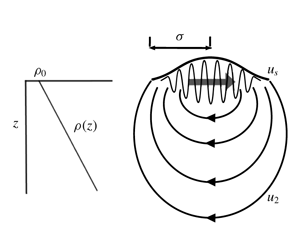
Realistic sea states do not consist of regular waves but are made up of wavepackets (Longuet-Higgins Reference Longuet-Higgins1984), a feature which is equivalent to a linear superposition of waves with different wavenumbers and frequencies. Since Stokes drift depends on the square of the local wave amplitude, its associated mass transport becomes horizontally divergent on the packet scale. Longuet-Higgins & Stewart (Reference Longuet-Higgins and Stewart1962) demonstrated that a deep return flow forms in response to this divergence. The total Lagrangian velocity is given by the sum of the Stokes drift and the induced return flow ( $\boldsymbol{u}_{L}=\boldsymbol{u}_{2}+\boldsymbol{u}_{S}$, e.g. Bühler (Reference Bühler2014)). For surface wavepackets in infinitely deep water, the Lagrangian-mean mass transport is zero (e.g. McIntyre Reference McIntyre1980). The Stokes drift is localised near the surface while the return flow is more persistent with depth, so that packets induce a depth-dependent mass transport (e.g. van den Bremer & Taylor Reference van den Bremer and Taylor2016). Due to directional spreading of the underlying wave spectrum about a peak wavenumber, wavepackets frequently exhibit localisation in the spanwise direction, which may considerably reduce the magnitude of the return flow and its associated displacement (e.g. van den Bremer & Taylor Reference van den Bremer and Taylor2015). Recently, Haney & Young (Reference Haney and Young2017) examined the propagation of a wavepacket on a stratified ocean, showing that density stratification significantly distorts the return flow.
In this paper, we investigate the Lagrangian transport associated with an isolated spanwise-localised (or three-dimensional) non-dissipating surface gravity wavepacket, considering unstratified and stratified oceans in turn, and focussing on the net displacements induced by the return flow. We emphasise that the model of an isolated wavepacket we consider is mainly of theoretical interest and not directly applicable to the real ocean. It is intended to provide general insight into subtle features of the displacements and potentially provide a benchmark against which to test the codes of more realistic sea-state models.
We assume throughout that directional spreading is relatively weak, so that the packet’s width is greater than or equal to its length in the direction of propagation. We examine wavetrains which are quasi-monochromatic, that is, with narrow-banded spectra. We also assume the surface waves have wavelengths much smaller than the water depth (i.e. are deep-water waves). We do not place such a restriction on the packet’s characteristic length scale relative to the depth, and thus on the scale of the return flow. For an unstratified ocean, we use perturbation methods to demonstrate that the net displacement of particles by the return flow is finite and depth-independent for a spanwise-infinite wavepacket (two-dimensional), but vanishes altogether for a spanwise-localised (three-dimensional) packet. In doing so, we correct erroneous numerical predictions by van den Bremer & Taylor (Reference van den Bremer and Taylor2016) of more complex displacement profiles in two dimensions and by van den Bremer & Taylor (Reference van den Bremer and Taylor2015) of small yet non-zero displacements in three dimensions. We resolve this contrast between two dimensions and three dimensions by exploring displacements over finite time intervals. While displacement underneath a 3-D wavepacket is initially two-dimensional-like (increasing in magnitude), an opposing part of the return flow brings a particle back to its original position at later times. This opposing part of the flow forms only in three dimensions, when the flow may return around as well as beneath the packet. Reversal of the particle displacement occurs at a time that is proportional to the packet’s width, hence much later for almost-2-D packets.
For a stratified ocean, we show that the net displacement profile by the return flow is a slowly oscillatory function of depth in two dimensions, with a wavelength depending on the ratio of buoyancy frequency  $N$ to the surface wave group velocity
 $c_{g,0}$. Large net displacements are predicted when the wavenumber
 $N/c_{g,0}$ is close to an integer multiple of
 $\unicode[STIX]{x03C0}/d$ (where
 $d$ is the ocean depth), corresponding to an exact resonance between
 $c_{g,0}$ and the phase velocity of an internal wave with zero horizontal wavenumber. In three dimensions, the net displacement remains zero even in the presence of stratification.
This paper is laid out as follows. First, § 2 examines the unstratified case, distinguishes net displacement in two dimensions (§ 2.2) and three dimensions (§ 2.3) and studies the transition between them over finite times (§ 2.4). Second, § 3 addresses the stratified case. We examine the implications of our results in § 4 and draw conclusions. Appendix A explores the influence of the second-order set-down of the free surface on net displacement, and appendix B considers the otherwise neglected impact of leading-order wave dispersion.
2 Unstratified flow
2.1 Governing equations
We begin by considering the unstratified case. A three-dimensional body of water of depth  $d$ and infinite lateral extent is assumed, with Cartesian coordinates (
 $x$,
 $y$,
 $z$), where
 $x$ and
 $y$ are the horizontal coordinates, and
 $z$ the vertical coordinate measured from the undisturbed water level upwards. Inviscid, incompressible and irrotational flow is assumed; hence the velocity can be written as the gradient of the velocity potential
 $\boldsymbol{u}=\unicode[STIX]{x1D735}\unicode[STIX]{x1D719}$. In addition to the no-flow condition at the bottom (
 $\unicode[STIX]{x2202}_{z}\unicode[STIX]{x1D719}=0$ at
 $z=-d$), the governing equation in the fluid interior (Laplace) and the kinematic and dynamic boundary conditions are
 $$\begin{eqnarray}\displaystyle (\unicode[STIX]{x2202}_{x}^{2}+\unicode[STIX]{x2202}_{y}^{2}+\unicode[STIX]{x2202}_{z}^{2})\unicode[STIX]{x1D719}=0,\quad \unicode[STIX]{x2202}_{z}\unicode[STIX]{x1D719}|_{z=h}=\unicode[STIX]{x2202}_{t}h+\unicode[STIX]{x1D735}_{H}\unicode[STIX]{x1D719}|_{z=h}\boldsymbol{\cdot }\unicode[STIX]{x1D735}_{H}h,\quad \unicode[STIX]{x2202}_{t}\unicode[STIX]{x1D719}|_{z=h}+gh+{\textstyle \frac{1}{2}}|\unicode[STIX]{x1D735}\unicode[STIX]{x1D719}|^{2}|_{z=h}=0, & & \displaystyle \nonumber\\ \displaystyle & & \displaystyle\end{eqnarray}$$
where the free surface elevation is denoted by  $z=h(x,y,t)$,
 $g$ is acceleration due to gravity and
 $\unicode[STIX]{x1D735}_{H}\equiv (\unicode[STIX]{x2202}_{x},\unicode[STIX]{x2202}_{y},0)$ is the horizontal gradient.
The wave amplitude is assumed small:  $\unicode[STIX]{x1D6FC}\equiv a_{0}k_{0}\ll 1$, where
 $a_{0}$ is the peak amplitude of the surface elevation and
 $k_{0}$ the wavenumber of the carrier wave. We solve the set (2.1) using a Stokes expansion and consider the first two orders, so that
 $\unicode[STIX]{x1D719}=\unicode[STIX]{x1D719}_{1}+\unicode[STIX]{x1D719}_{2}+\cdots \!$ and
 $h=h_{1}+h_{2}+\,\cdots \,$, with the subscript denoting the order in
 $\unicode[STIX]{x1D6FC}$.
2.1.1 First-order solutions:  $O(\unicode[STIX]{x1D6FC})$

We assume that the ocean is deep with respect to the waves ( $k_{0}d\gg 1$), and that the packet is quasi-monochromatic, weakly localised in the
 $x$ and
 $y$ directions, and propagates along the
 $x$-axis, so that the first-order solution takes the form
 $$\begin{eqnarray}\displaystyle & \displaystyle h_{1}=\text{Re}[A_{0}(\unicode[STIX]{x1D700}\tilde{x},\unicode[STIX]{x1D700}Ry,\unicode[STIX]{x1D700}^{2}t)\text{e}^{\text{i}\unicode[STIX]{x1D703}(x,t)}]+O(\unicode[STIX]{x1D6FC}\unicode[STIX]{x1D700}), & \displaystyle\end{eqnarray}$$
 $$\begin{eqnarray}\displaystyle & \displaystyle \unicode[STIX]{x1D719}_{1}=\text{Re}\left[-\frac{\text{i}\unicode[STIX]{x1D714}_{0}}{k_{0}}A_{0}(\unicode[STIX]{x1D700}\tilde{x},\unicode[STIX]{x1D700}Ry,\unicode[STIX]{x1D700}^{2}t)\text{e}^{\text{i}\unicode[STIX]{x1D703}(x,t)}\text{e}^{k_{0}z}\right]+O(\unicode[STIX]{x1D6FC}\unicode[STIX]{x1D700}), & \displaystyle\end{eqnarray}$$
 $\unicode[STIX]{x1D703}=k_{0}x-\unicode[STIX]{x1D714}_{0}t$ with
 $\unicode[STIX]{x1D714}_{0}=\sqrt{gk_{0}}$ the angular frequency, and
 $\tilde{x}\equiv x-c_{g,0}t$ is the coordinate in a frame moving at the group velocity
 $c_{g,0}=\unicode[STIX]{x1D714}_{0}/(2k_{0})$. The amplitude scale
 $a_{0}$ is taken as the envelope maximum
 $\sup |A_{0}|$. Wavepacket scales are captured by the bandwidth parameter
 $\unicode[STIX]{x1D700}\equiv (2k_{0}\unicode[STIX]{x1D70E}_{x})^{-1}\ll 1$ and aspect ratio
 $R\equiv \unicode[STIX]{x1D70E}_{x}/\unicode[STIX]{x1D70E}_{y}$, where
 $\unicode[STIX]{x1D70E}_{x}$ and
 $\unicode[STIX]{x1D70E}_{y}$ are the characteristic packet scales in
 $x$ (length) and in
 $y$ (width), respectively. The limit
 $\unicode[STIX]{x1D700}\rightarrow 0$ at fixed
 $R$ recovers the case of a periodic wave. Throughout this paper, we consider only
 $0\leqslant R\leqslant 1$, so that packets are never longer than they are wide; a 2-D packet corresponds to
 $R=0$ and a round packet to
 $R=1$. The
 $O(\unicode[STIX]{x1D6FC}\unicode[STIX]{x1D700})$ terms in (2.2a), (2.2b) are not needed to compute the leading-order wave-induced forcing, but must be examined when assessing effects of wave dispersion arising on a time scale
 $\unicode[STIX]{x1D700}^{2}t=O(1)$ (see appendix B).
The Stokes drift is a wave property in the standard sense that it can be calculated directly from the linear solutions (2.2) as
 $$\begin{eqnarray}\displaystyle \boldsymbol{u}_{S}=\overline{\unicode[STIX]{x0394}\boldsymbol{x}_{1}\boldsymbol{\cdot }\unicode[STIX]{x1D735}\boldsymbol{u}_{1}}=k_{0}\left(\unicode[STIX]{x1D714}_{0}|A_{0}|^{2},0,-{\textstyle \frac{3}{2}}\unicode[STIX]{x1D700}c_{g,0}\unicode[STIX]{x2202}_{\tilde{x}}|A_{0}|^{2}\right)\text{e}^{2k_{0}z}+O(\unicode[STIX]{x1D6FC}^{2}\unicode[STIX]{x1D700}^{2}), & & \displaystyle\end{eqnarray}$$
where the overbar represents an average over the wave phase, and  $\unicode[STIX]{x0394}\boldsymbol{x}_{1}=\int \boldsymbol{u}_{1}\,\text{d}t$.
2.1.2 Second-order solutions: $O(\unicode[STIX]{x1D6FC}^{2})$

The return flow is found by solving the wave-averaged governing equations at second order in steepness. Expanding (2.1b,c) about the undisturbed level  $z=0$ up to quadratic terms and wave averaging yields forcing equations for the Eulerian-mean flow and wave-averaged free surface (cf. Longuet-Higgins & Stewart Reference Longuet-Higgins and Stewart1962; McAllister et al. Reference McAllister, Adcock, Taylor and van den Bremer2018),
 $$\begin{eqnarray}\displaystyle & \displaystyle \left(\frac{1}{g}\unicode[STIX]{x2202}_{t}^{2}+\unicode[STIX]{x2202}_{z}\right)\unicode[STIX]{x1D719}_{2}=\unicode[STIX]{x1D735}_{H}\boldsymbol{\cdot }\overline{(\boldsymbol{u}_{1}h_{1})}\left.-\overline{\frac{1}{g}\unicode[STIX]{x2202}_{t}\left(h_{1}\unicode[STIX]{x2202}_{tz}\unicode[STIX]{x1D719}_{1}+\frac{1}{2}|\unicode[STIX]{x1D735}\unicode[STIX]{x1D719}_{1}|^{2}\right)}\right|_{z=0}, & \displaystyle\end{eqnarray}$$
 $$\begin{eqnarray}\displaystyle & \displaystyle h_{2}=-\frac{1}{g}\left.\left(\unicode[STIX]{x2202}_{t}\unicode[STIX]{x1D719}_{2}+\overline{\left(h_{1}\unicode[STIX]{x2202}_{tz}\unicode[STIX]{x1D719}_{1}+\frac{1}{2}|\unicode[STIX]{x1D735}\unicode[STIX]{x1D719}_{1}|^{2}\right)}\right)\right|_{z=0}, & \displaystyle\end{eqnarray}$$
where we focus on mean quantities only. The  $\unicode[STIX]{x2202}_{t}h_{2}$ term in (2.1b) has been eliminated using
 $\unicode[STIX]{x2202}_{t}$ (2.1c). The first term on the right of (2.4) is the forcing due to the horizontal divergence of the transport associated with the waves. In the Eulerian-mean description used here, the transport is confined to the layer
 $-h\leqslant z\leqslant h$ spanning from the troughs to the crests of the waves, and is given by
 $\overline{\boldsymbol{u}_{1}h_{1}}=\boldsymbol{M}$, say, to leading order. In the Lagrangian-mean description it is distributed over a deeper layer of depth
 ${\sim}k_{0}^{-1}$ as the Stokes drift, again to leading order. Thus
 $$\begin{eqnarray}\displaystyle \boldsymbol{M}\equiv \overline{(\boldsymbol{u}_{1}h_{1})}=\int _{-d}^{0}\boldsymbol{u}_{S}\,\text{d}z. & & \displaystyle\end{eqnarray}$$
We refer to  $\boldsymbol{M}$ in this paper as the Stokes transport. The second term on the right-hand side of (2.4) can be understood as the effect of the set-down of the wave-averaged free surface
 $h_{2}$ on the return flow. In deep water
 $(k_{0}d\gg 1)$, this set-down does not contribute to the forcing of the return flow to leading order, because the linear polarisation relationships for deep-water waves imply that
 $$\begin{eqnarray}\displaystyle \overline{\left(h_{1}\unicode[STIX]{x2202}_{tz}\unicode[STIX]{x1D719}_{1}+{\textstyle \frac{1}{2}}|\unicode[STIX]{x1D735}\unicode[STIX]{x1D719}_{1}|^{2}\right)}=0\quad \text{at }z=0, & & \displaystyle\end{eqnarray}$$
to leading order, as can be seen by substitution from (2.2) after setting  $\unicode[STIX]{x1D700}=0$. Furthermore, the double time derivative on the left of (2.4) can be ignored when
 $k_{0}d\gg 1$, so the return flow arises solely from the divergence of the Stokes transport (a rigid-lid approximation, see also the discussion in appendix A). Equation (2.4) then simplifies to
 $$\begin{eqnarray}\displaystyle \unicode[STIX]{x2202}_{z}\unicode[STIX]{x1D719}_{2}(\tilde{x},y,0)=\unicode[STIX]{x2202}_{\tilde{x}}M+O(\unicode[STIX]{x1D6FC}^{2}\unicode[STIX]{x1D700}^{2}), & & \displaystyle\end{eqnarray}$$
where  $M$ is the
 $x$-component of
 $\boldsymbol{M}$.
2.2 Unstratified flow in two dimensions
For two-dimensional flows induced by spanwise-infinite wavepackets, we make use of the streamfunction  $\unicode[STIX]{x1D713}_{2}$, implicitly defined by
 $\boldsymbol{u}_{2}=\unicode[STIX]{x1D735}\times (\unicode[STIX]{x1D713}_{2}\,\hat{\boldsymbol{y}})$ and satisfying a Laplace boundary-value problem. The surface value of the streamfunction is the Stokes transport, and the ocean floor is a streamline
 $$\begin{eqnarray}\displaystyle (\unicode[STIX]{x2202}_{\tilde{x}}^{2}+\unicode[STIX]{x2202}_{z}^{2})\unicode[STIX]{x1D713}_{2}=0,\quad \unicode[STIX]{x1D713}_{2}(\tilde{x},0)=M,\quad \unicode[STIX]{x1D713}_{2}(\tilde{x},-d)=0. & & \displaystyle\end{eqnarray}$$
We are interested in the net (or long-time) displacement by the return flow, defined at any fixed value of  $x$ by
 $$\begin{eqnarray}\displaystyle \unicode[STIX]{x0394}x=\int _{-\infty }^{\infty }u_{2}\,\text{d}t=\frac{1}{c_{g,0}}\int _{-\infty }^{\infty }u_{2}\,\text{d}\tilde{x}, & & \displaystyle\end{eqnarray}$$
where the second equality makes use of the translating reference frame of the packet. We can compute the net displacement (2.10) without explicitly evaluating  $\unicode[STIX]{x1D713}_{2}$. First, we integrate (2.9) over all
 $\tilde{x}$, noting that the vertical velocity
 $\unicode[STIX]{x2202}_{\tilde{x}}\unicode[STIX]{x1D713}_{2}$ is zero at infinity, which reduces (2.9a) to the ordinary differential equation
 $$\begin{eqnarray}\displaystyle \frac{\text{d}^{2}}{\text{d}z^{2}}\int _{-\infty }^{\infty }\unicode[STIX]{x1D713}_{2}\,\text{d}\tilde{x}=0,\quad \text{with }\left.\int _{-\infty }^{\infty }\unicode[STIX]{x1D713}_{2}\,\text{d}\tilde{x}\right|_{z=0}=\int _{-\infty }^{\infty }M\,\text{d}\tilde{x},\quad \left.\int _{-\infty }^{\infty }\unicode[STIX]{x1D713}_{2}\,\text{d}\tilde{x}\right|_{z=-d}=0, & & \displaystyle \nonumber\\ \displaystyle & & \displaystyle\end{eqnarray}$$
as boundary conditions. The solution is
 $$\begin{eqnarray}\displaystyle \int _{-\infty }^{\infty }\unicode[STIX]{x1D713}_{2}(\tilde{x},z)\,\text{d}\tilde{x}=\left(\frac{z+d}{d}\right)\int _{-\infty }^{\infty }M\,\text{d}\tilde{x}, & & \displaystyle\end{eqnarray}$$
and the net displacement is deduced by dividing by  $c_{g,0}$ and taking the negative
 $z$-derivative (using (2.10) and
 $u_{2}=-\unicode[STIX]{x2202}_{z}\unicode[STIX]{x1D713}_{2}$),
 $$\begin{eqnarray}\displaystyle \unicode[STIX]{x0394}x=-\frac{1}{c_{g,0}}\unicode[STIX]{x2202}_{z}\int _{-\infty }^{\infty }\unicode[STIX]{x1D713}_{2}(\tilde{x},z)\,\text{d}\tilde{x}=-\frac{1}{c_{g,0}d}\int _{-\infty }^{\infty }M\,\text{d}\tilde{x}. & & \displaystyle\end{eqnarray}$$
We thus obtain the perhaps surprising result that the net displacement by the return flow is independent of depth. The displacement is finite and negative, unless the ocean depth is truly infinite (not just  $k_{0}d\gg 1$), when it goes to zero. Note that (2.13) is valid for any narrow-banded, unidirectional Stokes transport
 $M$.
The net Lagrangian displacement  $\unicode[STIX]{x0394}x_{L}\equiv \unicode[STIX]{x0394}x+\unicode[STIX]{x0394}x_{S}$ is depth dependent, and is obtained by integrating (2.3) with respect to time and adding to (2.13),
 $$\begin{eqnarray}\displaystyle \hspace{-5.0pt}\unicode[STIX]{x0394}x_{L}=\frac{\unicode[STIX]{x1D6FC}^{2}\sqrt{\unicode[STIX]{x03C0}}}{k_{0}}\left(2k_{0}\unicode[STIX]{x1D70E}_{x}\text{e}^{2k_{0}z}-\frac{\unicode[STIX]{x1D70E}_{x}}{d}\right), & & \displaystyle\end{eqnarray}$$
where we have assumed a Gaussian packet  $A_{0}=a_{0}\exp (-\tilde{x}^{2}/(2\unicode[STIX]{x1D70E}_{x}^{2}))$, resulting in the Stokes transport
 $M=\unicode[STIX]{x1D714}_{0}a_{0}^{2}\exp (-\tilde{x}^{2}/\unicode[STIX]{x1D70E}_{x}^{2})/2$, and
 $\unicode[STIX]{x1D6FC}=a_{0}k_{0}$ denotes wave steepness, as before. Lagrangian particles are displaced forwards above a certain depth and rearwards beneath it. Depth integrating (2.14) from
 $-d$ to
 $0$ gives the total volume transported by the Lagrangian flow, which vanishes in the limit
 $k_{0}d\gg 1$ considered here. Whenever we assume Gaussian packets, displacements scaled by
 $\unicode[STIX]{x1D6FC}^{2}\sqrt{\unicode[STIX]{x03C0}}/k_{0}$ will be denoted by a star,
 $$\begin{eqnarray}\displaystyle \unicode[STIX]{x0394}x^{\ast }\equiv k_{0}\unicode[STIX]{x0394}x/(\unicode[STIX]{x1D6FC}^{2}\sqrt{\unicode[STIX]{x03C0}}),\quad \unicode[STIX]{x0394}x_{S}^{\ast }\equiv k_{0}\unicode[STIX]{x0394}x_{S}/(\unicode[STIX]{x1D6FC}^{2}\sqrt{\unicode[STIX]{x03C0}}),\quad \unicode[STIX]{x0394}x_{L}^{\ast }\equiv k_{0}\unicode[STIX]{x0394}x_{L}/(\unicode[STIX]{x1D6FC}^{2}\sqrt{\unicode[STIX]{x03C0}}),\quad \qquad & & \displaystyle\end{eqnarray}$$
so that  $\unicode[STIX]{x0394}x^{\ast }=-1/d^{\ast }$ with
 $d^{\ast }=d/\unicode[STIX]{x1D70E}_{x}$.
2.3 Unstratified flow in three dimensions
In three dimensions, we evaluate the net displacement in two different ways. First, we use a double Fourier transform in  $\tilde{x}$ and
 $y$ to obtain the potential
 $$\begin{eqnarray}\displaystyle \unicode[STIX]{x1D719}_{2}(\tilde{x},y,z)=\frac{1}{4\unicode[STIX]{x03C0}^{2}}\text{Re}\iint _{\mathbb{R}^{2}}\frac{\text{i}k\hat{M}}{\sqrt{k^{2}+l^{2}}}\frac{\cosh ((z+d)\sqrt{k^{2}+l^{2}})}{\sinh (d\sqrt{k^{2}+l^{2}})}\text{e}^{\text{i}k\tilde{x}}\text{e}^{\text{i}ly}\,\text{d}k\,\text{d}l, & & \displaystyle\end{eqnarray}$$
where  $\hat{M}(k,l)$ is the Fourier transform of
 $M(\tilde{x},y)$. To find the net displacement, we take the
 $x$-derivative of (2.16) to obtain
 $u_{2}$ and integrate over all time (here
 $\tilde{x}$), resulting in a delta function in
 $k$. This forces the integral to evaluate to zero (unless
 $l=0$),
 $$\begin{eqnarray}\displaystyle \unicode[STIX]{x0394}x=-\frac{1}{2\unicode[STIX]{x03C0}c_{g,0}}\text{Re}\iint _{\mathbb{R}^{2}}\unicode[STIX]{x1D6FF}(k)\frac{k^{2}\hat{M}}{\sqrt{k^{2}+l^{2}}}\frac{\cosh ((z+d)\sqrt{k^{2}+l^{2}})}{\sinh (d\sqrt{k^{2}+l^{2}})}\text{e}^{\text{i}ly}\,\text{d}k\,\text{d}l=0. & & \displaystyle\end{eqnarray}$$
This result is in stark contrast with the negative, depth-independent net displacement in two dimensions (2.13). Second, we can also obtain this result from irrotationality of the return flow,
 $$\begin{eqnarray}\displaystyle \unicode[STIX]{x2202}_{y}w_{2}=\unicode[STIX]{x2202}_{z}v_{2},\quad \unicode[STIX]{x2202}_{z}u_{2}=\unicode[STIX]{x2202}_{x}w_{2},\quad \unicode[STIX]{x2202}_{y}u_{2}=\unicode[STIX]{x2202}_{x}v_{2}. & & \displaystyle\end{eqnarray}$$
Integrating (2.18b,c) over all time (equivalently,  $\tilde{x}$), and assuming the velocity components
 $v_{2}$ and
 $w_{2}$ decay far from the packet
 $(|\tilde{x}|\rightarrow \infty )$, we obtain the conditions
 $$\begin{eqnarray}\displaystyle \unicode[STIX]{x2202}_{z}\unicode[STIX]{x0394}x=0,\quad \unicode[STIX]{x2202}_{y}\unicode[STIX]{x0394}x=0, & & \displaystyle\end{eqnarray}$$
which together imply the net displacement  $\unicode[STIX]{x0394}x$ is at most a constant. As we also require the flow to decay as
 $|y|\rightarrow \infty$, we immediately obtain the result that
 $\unicode[STIX]{x0394}x=0$.
Physical insight into this 2-D–3-D contrast may be obtained from mass balance arguments. Depth integrating the incompressibility condition ( $\unicode[STIX]{x1D735}\boldsymbol{\cdot }\boldsymbol{u}_{2}=0$), and using (2.6) and (2.8), we obtain in three dimensions
 $$\begin{eqnarray}\displaystyle \unicode[STIX]{x2202}_{\tilde{x}}\int _{-d}^{0}(u_{2}+u_{S})\,\text{d}z=-\unicode[STIX]{x2202}_{y}\int _{-d}^{0}v_{2}\,\text{d}z, & & \displaystyle\end{eqnarray}$$
where we have also used the boundary condition for  $w_{2}$ at the bottom and rewritten
 $M$ as the vertical integral of the Stokes drift, as in (2.6). Thus at each time
 $t$, the divergence of the Lagrangian transport in the propagation direction is counterbalanced by a gradient of transport in the
 $y$ direction. In fact, the
 $yz$-area integral of the Lagrangian velocity is zero at each
 $t$, which may be seen by
 $y$-integrating (2.20) and again noting the decay at large
 $|\tilde{x}|$ and
 $|y|$. Despite the net return-flow displacement
 $\unicode[STIX]{x0394}x$ being zero at any point, its
 $yz$-area integral must balance the
 $yz$-area integral of the Stokes drift displacement, which is non-zero since the Stokes drift is depth limited and inherits the envelope decay of the packet, decaying rapidly in both
 $y$ and
 $z$. Mathematically, the time and area integrals do not commute – to put it more starkly,
 $\int \int \unicode[STIX]{x0394}x\,\text{d}y\,\text{d}z$ is essentially zero times infinity, hence undefined. This result is independent of the functional form of
 $M$. We will now explore displacements over finite time intervals.
2.4 Finite-time displacement and the 2-D–3-D transition
We define the symmetric finite-time return-flow displacement (finite-time displacement, for brevity) as the following symmetric time integral evaluated at  $x=y=0$ over the time interval
 $[-t_{\mathit{I}},t_{\mathit{I}}]$:
 $$\begin{eqnarray}\displaystyle \unicode[STIX]{x0394}x(t_{\mathit{I}},z,d)=\int _{-t_{\mathit{I}}}^{t_{\mathit{I}}}u_{2}\,\text{d}t=\frac{1}{c_{g,0}}\int _{-c_{g,0}t_{\mathit{I}}}^{c_{g,0}t_{\mathit{I}}}u_{2}\,\text{d}\tilde{x}, & & \displaystyle\end{eqnarray}$$
thereby examining a particle underneath the centre of the packet at  $t=0$. We display the arguments
 $(t_{\mathit{I}},z,d)$ on the left of (2.21) to distinguish the finite-time displacement from its long-time limit, denoted as before by
 $\unicode[STIX]{x0394}x$ without arguments. Recall that the long-time limit
 $\unicode[STIX]{x0394}x$ has no
 $z$-dependence, either in three dimensions when it is zero at each
 $(y,z)$, or in two dimensions when it is a non-zero constant. In this section we choose the Stokes transport
 $M$, and thereby its Fourier transform
 $\hat{M}$, to be Gaussian,
 $$\begin{eqnarray}\displaystyle M=\frac{\unicode[STIX]{x1D714}_{0}a_{0}^{2}}{2}\text{e}^{-\tilde{x}^{2}/\unicode[STIX]{x1D70E}_{x}^{2}}\text{e}^{-y^{2}/\unicode[STIX]{x1D70E}_{y}^{2}},\quad \hat{M}=\frac{\unicode[STIX]{x1D714}_{0}a_{0}^{2}\unicode[STIX]{x1D70E}_{x}\unicode[STIX]{x1D70E}_{y}\unicode[STIX]{x03C0}}{2}\text{e}^{-k^{2}\unicode[STIX]{x1D70E}_{x}^{2}/4}\text{e}^{-l^{2}\unicode[STIX]{x1D70E}_{y}^{2}/4}. & & \displaystyle\end{eqnarray}$$
Differentiating (2.16) with respect to  $\tilde{x}$ to obtain
 $u_{2}$ and integrating as in (2.21), we obtain after moving to the non-dimensional variables
 $\unicode[STIX]{x1D707}\equiv kc_{g,0}t_{\mathit{I}}$ and
 $\unicode[STIX]{x1D706}\equiv l\unicode[STIX]{x1D70E}_{y}$,
 $$\begin{eqnarray}\displaystyle \unicode[STIX]{x0394}x^{\ast }(\unicode[STIX]{x1D70F},z^{\ast },R,d^{\ast }) & = & \displaystyle \frac{-1}{2\unicode[STIX]{x03C0}^{3/2}\unicode[STIX]{x1D70F}}\text{Re}\iint _{\mathbb{R}^{2}}\frac{\unicode[STIX]{x1D707}\sin (\unicode[STIX]{x1D707})}{\sqrt{\unicode[STIX]{x1D707}^{2}+(R\unicode[STIX]{x1D70F})^{2}\unicode[STIX]{x1D706}^{2}}}\text{e}^{-\unicode[STIX]{x1D707}^{2}/(4\unicode[STIX]{x1D70F}^{2})}\text{e}^{-\unicode[STIX]{x1D706}^{2}/4}\nonumber\\ \displaystyle & & \displaystyle \times \,\frac{\cosh ((z^{\ast }+d^{\ast })\sqrt{\unicode[STIX]{x1D707}^{2}+(R\unicode[STIX]{x1D70F})^{2}\unicode[STIX]{x1D706}^{2}}/\unicode[STIX]{x1D70F})}{\sinh (d^{\ast }\sqrt{\unicode[STIX]{x1D707}^{2}+(R\unicode[STIX]{x1D70F})^{2}\unicode[STIX]{x1D706}^{2}}/\unicode[STIX]{x1D70F})}\,\text{d}\unicode[STIX]{x1D707}\,\text{d}\unicode[STIX]{x1D706},\end{eqnarray}$$
where we have replaced  $z$ by
 $z^{\ast }\equiv z/\unicode[STIX]{x1D70E}_{x}$,
 $d$ by
 $d^{\ast }\equiv d/\unicode[STIX]{x1D70E}_{x}$ and
 $t_{\mathit{I}}$ by
 $\unicode[STIX]{x1D70F}\equiv c_{g,0}t_{\mathit{I}}/\unicode[STIX]{x1D70E}_{x}$, i.e. the half-interval
 $t_{\mathit{I}}$ scaled by the packet translation time
 $\unicode[STIX]{x1D70E}_{x}/c_{g,0}$. As before, the aspect ratio
 $R\equiv \unicode[STIX]{x1D70E}_{x}/\unicode[STIX]{x1D70E}_{y}$ so that
 $R\rightarrow 0$ corresponds to two dimensions; and
 $\unicode[STIX]{x0394}x^{\ast }$ is scaled as in (2.15a).
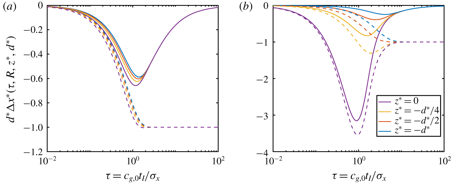
Scaled finite-time displacement at various depths, obtained from numerical integration of (2.23). Solid lines correspond to a 3-D flow with  $R=\unicode[STIX]{x1D70E}_{x}/\unicode[STIX]{x1D70E}_{y}=1/3$, and the dashed lines to a 2-D flow (
 $R=0$). Panel (a) shows the displacement for a shallower return flow (
 $d^{\ast }=0.5$, on the left), and (b) for a deeper return flow (
 $d^{\ast }=5$, on the right).

Figure 1 shows results obtained by numerical integration of (2.23) for particles at various depths in a 3-D flow ( $R=1/3$), and in a 2-D flow (
 $R=0$). We plot the scaled finite-time return-flow displacement
 $d^{\ast }\unicode[STIX]{x0394}x^{\ast }(\unicode[STIX]{x1D70F},R,z^{\ast },d^{\ast })$ (for brevity, we refer to this as the scaled finite-time displacement). The
 $\unicode[STIX]{x1D70F}$-axis is logarithmic to show the behaviour for very small and very large
 $\unicode[STIX]{x1D70F}$. Behaviour for small
 $\unicode[STIX]{x1D70F}$ is two-dimensional-like, while for large
 $\unicode[STIX]{x1D70F}$ the continuous lines (three-dimensional) tend towards zero and the dashed lines (two-dimensional) to
 $-1$, as previously discussed in (2.17) and (2.15a). The two panels compare a shallower return flow (
 $d^{\ast }=0.5$) and a deeper return flow (
 $d^{\ast }=5$). Whereas the 2-D finite-time displacement is very nearly monotonic for shallower return flows, it can overshoot near the surface for deeper return flows, reflecting strong negative displacement underneath the centre of the packet being partly cancelled, subsequently, by positive displacement near the surface at the packet’s leading and trailing edges. We have been unable to convert (2.23) into a more insightful form, so we consider the limiting case of a shallow return flow, corresponding to
 $d^{\ast }=d/\unicode[STIX]{x1D70E}_{x}\ll 1$. In this limit, the return flow’s vertical variation is negligible, and (2.23) takes the form
 $$\begin{eqnarray}\displaystyle \unicode[STIX]{x0394}x^{\ast }(\unicode[STIX]{x1D70F},R)=-\frac{2}{d^{\ast }\unicode[STIX]{x03C0}^{3/2}}\int _{0}^{\infty }\int _{0}^{\infty }\frac{\unicode[STIX]{x1D707}\sin (\unicode[STIX]{x1D707})}{\unicode[STIX]{x1D707}^{2}+(R\unicode[STIX]{x1D70F})^{2}\unicode[STIX]{x1D706}^{2}}\text{e}^{-\unicode[STIX]{x1D707}^{2}/(4\unicode[STIX]{x1D70F}^{2})}\text{e}^{-\unicode[STIX]{x1D706}^{2}/4}\,\text{d}\unicode[STIX]{x1D707}\,\text{d}\unicode[STIX]{x1D706}. & & \displaystyle\end{eqnarray}$$
The integral over  $\unicode[STIX]{x1D706}$ may be performed analytically, yielding a single integral over
 $\unicode[STIX]{x1D707}$,
 $$\begin{eqnarray}\displaystyle \unicode[STIX]{x0394}x^{\ast }(\unicode[STIX]{x1D70F},R)=-\frac{2}{d^{\ast }\sqrt{\unicode[STIX]{x03C0}}}\int _{0}^{\infty }\frac{\sin \unicode[STIX]{x1D707}}{\unicode[STIX]{x1D707}}\text{e}^{-\unicode[STIX]{x1D707}^{2}/(4\unicode[STIX]{x1D70F}^{2})}f(\unicode[STIX]{x1D707}/(2R\unicode[STIX]{x1D70F}))\,\text{d}\unicode[STIX]{x1D707}, & & \displaystyle\end{eqnarray}$$
where the function  $f(\unicode[STIX]{x1D709})\equiv \unicode[STIX]{x1D709}\exp (\unicode[STIX]{x1D709}^{2})\text{erfc}(\unicode[STIX]{x1D709})$ for an arbitrary argument
 $\unicode[STIX]{x1D709}$ captures how the finite-time displacement varies with
 $R$; its relevant small and large
 $R\unicode[STIX]{x1D70F}$ limits are
 $$\begin{eqnarray}\displaystyle \lim _{R\unicode[STIX]{x1D70F}\rightarrow 0}f\left(\frac{\unicode[STIX]{x1D707}}{2R\unicode[STIX]{x1D70F}}\right)=\frac{1}{\sqrt{\unicode[STIX]{x03C0}}},\quad \lim _{R\unicode[STIX]{x1D70F}\rightarrow \infty }f\left(\frac{\unicode[STIX]{x1D707}}{2R\unicode[STIX]{x1D70F}}\right)=0. & & \displaystyle\end{eqnarray}$$
We can split (2.25) into the sum of two integrals
 $$\begin{eqnarray}\displaystyle \unicode[STIX]{x0394}x^{\ast }(\unicode[STIX]{x1D70F},R) & = & \displaystyle -\frac{2}{d^{\ast }\sqrt{\unicode[STIX]{x03C0}}}\int _{0}^{\infty }\text{e}^{-\unicode[STIX]{x1D707}^{2}/(4\unicode[STIX]{x1D70F}^{2})}\frac{\sin \unicode[STIX]{x1D707}}{\unicode[STIX]{x1D707}}\left(f\left(\frac{\unicode[STIX]{x1D707}}{2R\unicode[STIX]{x1D70F}}\right)-\frac{1}{\sqrt{\unicode[STIX]{x03C0}}}\right)\text{d}\unicode[STIX]{x1D707}\nonumber\\ \displaystyle & & \displaystyle -\,\frac{2}{d^{\ast }\unicode[STIX]{x03C0}}\int _{0}^{\infty }\text{e}^{-\unicode[STIX]{x1D707}^{2}/(4\unicode[STIX]{x1D70F}^{2})}\frac{\sin \unicode[STIX]{x1D707}}{\unicode[STIX]{x1D707}}\,\text{d}\unicode[STIX]{x1D707},\end{eqnarray}$$
the latter of which equals the 2-D finite-time shallow return-flow displacement. To examine the long-time behaviour we take  $\unicode[STIX]{x1D70F}\gg 1$, so that the second term approaches
 $-1/d^{\ast }$ (cf. (2.15a), and the Gaussian in the first can be set to
 $1$. We examine the regime
 $R\ll 1$,
 $\unicode[STIX]{x1D70F}\gg 1$, when the displacement becomes a function of a single,
 $O(1)$ parameter,
 $\unicode[STIX]{x1D701}\equiv R\unicode[STIX]{x1D70F}=c_{g,0}t_{\mathit{I}}/\unicode[STIX]{x1D70E}_{y}$, corresponding to the half-interval
 $t_{\mathit{I}}$ scaled on the packet width
 $\unicode[STIX]{x1D70E}_{y}$ rather than its length
 $\unicode[STIX]{x1D70E}_{x}$. We obtain
 $$\begin{eqnarray}\displaystyle \unicode[STIX]{x0394}x^{\ast }(\unicode[STIX]{x1D701})=-\frac{2}{d^{\ast }\sqrt{\unicode[STIX]{x03C0}}}\int _{0}^{\infty }\frac{\sin \unicode[STIX]{x1D707}}{\unicode[STIX]{x1D707}}\left(f\left(\frac{\unicode[STIX]{x1D707}}{2\unicode[STIX]{x1D701}}\right)-\frac{1}{\sqrt{\unicode[STIX]{x03C0}}}\right)\text{d}\unicode[STIX]{x1D707}-\frac{1}{d^{\ast }}. & & \displaystyle\end{eqnarray}$$
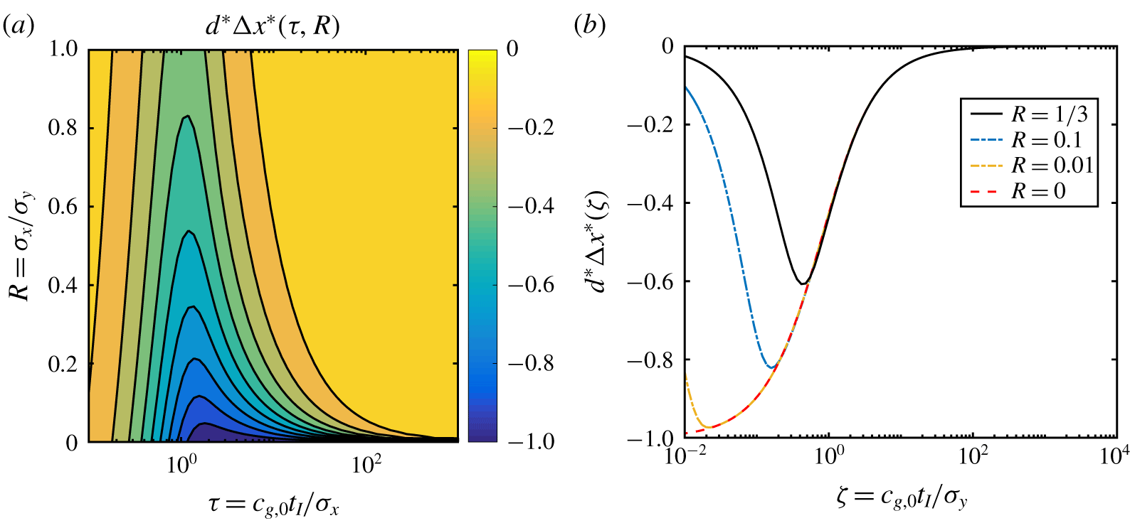
Figure 2(a) shows contours plots of the scaled finite-time displacement by a shallow return flow obtained by numerically integrating (2.21), demonstrating that the maximum negative displacement occurs for  $\unicode[STIX]{x1D70F}\sim 1$. From (2.28) and (2.26), it is clear that a transition between 2-D-like behaviour (
 $\unicode[STIX]{x1D701}\ll 1$) and 3-D-like behaviour (
 $\unicode[STIX]{x1D701}\gg 1$) occurs when
 $\unicode[STIX]{x1D701}\sim 1$ (
 $t_{\mathit{I}}\sim \unicode[STIX]{x1D70E}_{y}/c_{g,0}$). Two-dimensional-like behaviour can thus persist for arbitrarily large
 $\unicode[STIX]{x1D70F}$, given arbitrarily small amounts of localisation in
 $y$ (small
 $R$, or nearly unidirectional packets). Figure 2(b) compares numerical integration of (2.24) with numerical integration of its large-
 $\unicode[STIX]{x1D70F}$ limit (2.28).
Scaled finite-time displacement by shallow unstratified flow: contour plot as a function of aspect ratio  $R$ and half-interval
 $\unicode[STIX]{x1D70F}$, obtained by numerically integrating (2.25) (a), and displacement obtained by numerical integration of (2.25) for three aspect ratios (continuous black and dash-dotted blue and yellow lines, respectively) and (2.28) (red dashed line) as a function of
 $\unicode[STIX]{x1D701}=R\unicode[STIX]{x1D70F}$ (b).

We note in passing that incorrect non-zero values of net return-flow displacements obtained from numerical integration in van den Bremer & Taylor (Reference van den Bremer and Taylor2016) (two-dimensional, infinite depth) and van den Bremer & Taylor (Reference van den Bremer and Taylor2015) (three-dimensional) resulted from insufficiently large limits on the integrals; these limits may need to be as large as  $\unicode[STIX]{x1D70F}\sim 10^{2}{-}10^{3}$ for the small
 $R$ values used therein.
3 Stratified flow
3.1 Governing equations
In this section, we consider propagation of surface waves on a stratified fluid. To include density stratification effects, we decompose the varying density as (Phillips Reference Phillips1977)
 $$\begin{eqnarray}\displaystyle \unicode[STIX]{x1D70C}=\unicode[STIX]{x1D70C}_{0}\left(1+\frac{1}{g}\int _{z}^{0}N^{2}(z^{\prime })\,\text{d}z^{\prime }-\frac{b}{g}\right), & & \displaystyle\end{eqnarray}$$
where  $b(x,y,z,t)=-g\unicode[STIX]{x0394}\unicode[STIX]{x1D70C}/\unicode[STIX]{x1D70C}_{0}$ is the buoyancy perturbation, and
 $N$ is the buoyancy frequency, which we assume to be constant. Invoking the Boussinesq approximation by neglecting density differences unless they result in a body force through multiplication by
 $g$, the governing equations are (e.g. Haney & Young Reference Haney and Young2017)
 $$\begin{eqnarray}\displaystyle \unicode[STIX]{x1D735}\boldsymbol{\cdot }\boldsymbol{u}=0,\quad \unicode[STIX]{x2202}_{t}\boldsymbol{u}+\boldsymbol{u}\boldsymbol{\cdot }\unicode[STIX]{x1D735}\boldsymbol{u}=-\unicode[STIX]{x1D735}p+b\hat{\boldsymbol{z}},\quad \unicode[STIX]{x2202}_{t}b+\boldsymbol{u}\boldsymbol{\cdot }\unicode[STIX]{x1D735}b+wN^{2}=0, & & \displaystyle\end{eqnarray}$$
where  $p$ is the departure from hydrostatic pressure. The system (3.2) must be solved subject to dynamic and kinematic boundary conditions at the surface. Only the dynamic boundary condition (
 $p_{tot}=0$ at
 $z=h(x,y,t)$, where
 $p_{tot}$ is the total pressure) is modified by density stratification, and we have, correct to second order (Haney & Young Reference Haney and Young2017),
 $$\begin{eqnarray}\displaystyle w=\unicode[STIX]{x2202}_{t}h+\boldsymbol{u}_{H}\boldsymbol{\cdot }\unicode[STIX]{x1D735}_{H}h|_{z=0},\quad p+h\unicode[STIX]{x2202}_{z}p=gh+N^{2}h^{2}/2|_{z=0}. & & \displaystyle\end{eqnarray}$$
We solve the set (3.2)–(3.3) using a Stokes expansion as before and consider directly the 3-D case.
3.1.1 First-order solutions: $O(\unicode[STIX]{x1D6FC})$

Following Haney & Young (Reference Haney and Young2017), we neglect the buoyancy force and the vorticity it generates in the first-order equations. From the linearised equation (3.2c) and boundary condition (3.3a), we have  $b_{1}\sim -N^{2}h_{1}$. Taking the curl of the linearised (3.2b), we thus obtain for the non-dimensional vorticity
 $$\begin{eqnarray}\displaystyle \frac{|\unicode[STIX]{x1D735}\times \boldsymbol{u}_{1}|}{k_{0}a_{0}\unicode[STIX]{x1D714}_{0}}\sim \frac{|(\hat{\boldsymbol{z}}\times \unicode[STIX]{x1D735}_{H})b_{1}|}{k_{0}a_{0}\unicode[STIX]{x1D714}_{0}^{2}}\sim \frac{N^{2}}{\unicode[STIX]{x1D714}_{0}^{2}}, & & \displaystyle\end{eqnarray}$$
from which it is evident that vorticity is small provided  $(N/\unicode[STIX]{x1D714}_{0})^{2}$ is small. For surface gravity waves in the ocean,
 $(N/\unicode[STIX]{x1D714}_{0})^{2}$ is at most
 $O(10^{-3})$, and so the linear waves may be treated as irrotational by ignoring the small
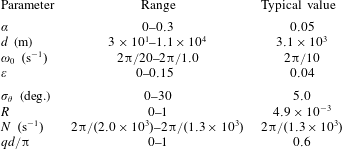
 $b_{1}$ (see table 1 for typical parameter values).
3.1.2 Second-order solutions: $O(\unicode[STIX]{x1D6FC}^{2})$

At second order we retain the wave-averaged buoyancy, and so the Eulerian-mean flow is not irrotational. Wave averaging the set (3.2), and defining the appropriate Bernoulli function to be  $\unicode[STIX]{x1D71B}_{2}\equiv p_{2}+\overline{|\boldsymbol{u}_{1}|^{2}}/2$, the Eulerian-mean flow equations are (Haney & Young Reference Haney and Young2017)
 $$\begin{eqnarray}\displaystyle \unicode[STIX]{x1D735}\boldsymbol{\cdot }\boldsymbol{u}_{2}=0,\quad \unicode[STIX]{x2202}_{t}\boldsymbol{u}_{2}=-\unicode[STIX]{x1D735}\unicode[STIX]{x1D71B}_{2}+b_{2}\hat{\boldsymbol{z}},\quad \unicode[STIX]{x2202}_{t}b_{2}=-w_{2}N^{2}. & & \displaystyle\end{eqnarray}$$
We have neglected  $\overline{\boldsymbol{u}_{1}\boldsymbol{\cdot }\unicode[STIX]{x1D735}b_{1}}$ in (3.5c); by (3.4) this is
 $O((N/\unicode[STIX]{x1D714}_{0})^{2})$ smaller than the other terms. Taking propagation along the
 $x$-axis, and using (2.7) with
 $p_{1}$ in place of
 $-\unicode[STIX]{x2202}_{t}\unicode[STIX]{x1D719}_{1}$ since the waves are irrotational, we may rewrite (3.3b) using the Bernoulli function as
 $$\begin{eqnarray}\displaystyle w_{2}|_{z=0}=\unicode[STIX]{x2202}_{t}h_{2}+\unicode[STIX]{x2202}_{x}M,\quad \unicode[STIX]{x1D71B}_{2}|_{z=0}=gh_{2}+N^{2}\overline{{h_{1}}^{2}}/2, & & \displaystyle\end{eqnarray}$$
where  $M$ is the
 $x$-component of
 $\boldsymbol{M}$ defined in (2.6). After eliminating all variables in favour of the vertical velocity
 $w_{2}$, and making the rigid-lid approximation in (3.6a) (as in (2.8)), the original problem (3.5) reduces to solving an evolution equation for
 $w_{2}$ subject to the surface forcing and no-flow bottom boundary condition,
 $$\begin{eqnarray}\displaystyle ((\unicode[STIX]{x2202}_{\tilde{x}}-\unicode[STIX]{x1D702})^{2}(\unicode[STIX]{x2202}_{x}^{2}+\unicode[STIX]{x2202}_{y}^{2}+\unicode[STIX]{x2202}_{z}^{2})+q^{2}(\unicode[STIX]{x2202}_{x}^{2}+\unicode[STIX]{x2202}_{y}^{2}))w_{2}=0,\quad w_{2}|_{z=0}=\unicode[STIX]{x2202}_{\tilde{x}}M,\quad w|_{z=-d}=0,\quad \qquad & & \displaystyle\end{eqnarray}$$
where  $c_{g,0}\unicode[STIX]{x1D702}$ is a small, positive growth rate which we take to zero from above, ensuring that any radiated internal waves appear in the packet’s wake, and
 $q\equiv N/c_{g,0}$ is the buoyancy wavenumber. By assuming the packet amplitude has been slowly growing from
 $t=-\infty$ (i.e.
 $A_{0}(\tilde{x},y)\text{e}^{c_{g,0}\unicode[STIX]{x1D702}t}$), in the packet’s reference frame we have
 $\unicode[STIX]{x2202}_{t}=-c_{g,0}(\unicode[STIX]{x2202}_{\tilde{x}}+\unicode[STIX]{x1D702})$. Throughout, we take
 $q$ (hence
 $N$) to be constant. The vertical velocity
 $w_{2}$ is obtained from (3.7) as the Fourier transform
 $$\begin{eqnarray}\displaystyle w_{2}(\tilde{x},y,z,d,q)=\frac{1}{4\unicode[STIX]{x03C0}^{2}}\lim _{\unicode[STIX]{x1D702}\rightarrow 0^{+}}\iint _{\mathbb{R}^{2}}\text{i}k\hat{M}\frac{\sinh ((z+d)|\boldsymbol{k}|\unicode[STIX]{x1D6FD}_{\unicode[STIX]{x1D702},q}(k))}{\sinh (d|\boldsymbol{k}|\unicode[STIX]{x1D6FD}_{\unicode[STIX]{x1D702},q}(k))}\text{e}^{\text{i}k\tilde{x}}\text{e}^{\text{i}ly}\,\text{d}k\,\text{d}l, & & \displaystyle\end{eqnarray}$$
where we have adopted the compact notation
 $$\begin{eqnarray}\displaystyle |\boldsymbol{k}|\equiv \sqrt{k^{2}+l^{2}},\quad \unicode[STIX]{x1D6FD}_{\unicode[STIX]{x1D702},q}(k)\equiv \sqrt{\frac{(k+\text{i}\unicode[STIX]{x1D702})^{2}-q^{2}}{(k+\text{i}\unicode[STIX]{x1D702})^{2}}}. & & \displaystyle\end{eqnarray}$$
To obtain the horizontal component  $u_{2}$ from
 $w_{2}$ we first link vorticity generation to the rotated gradient of buoyancy by taking the curl of momentum equation (3.5b),
 $$\begin{eqnarray}\displaystyle \unicode[STIX]{x2202}_{t}(\unicode[STIX]{x1D735}\times \boldsymbol{u}_{2})=-(\hat{\boldsymbol{z}}\times \unicode[STIX]{x1D735}_{H})b_{2}=(\unicode[STIX]{x2202}_{y}b_{2},-\unicode[STIX]{x2202}_{x}b_{2},0), & & \displaystyle\end{eqnarray}$$
from which it immediately follows that the vertical vorticity component is time independent. Assuming this vanishes,  $\unicode[STIX]{x2202}_{y}u_{2}-\unicode[STIX]{x2202}_{\tilde{x}}v_{2}=0$; combining this with the incompressibility condition (3.5a) leads to a Poisson-like equation relating
 $u_{2}$ to
 $w_{2}$,
 $$\begin{eqnarray}\displaystyle -(\unicode[STIX]{x2202}_{\tilde{x}}^{2}+\unicode[STIX]{x2202}_{y}^{2})u_{2}=\unicode[STIX]{x2202}_{\tilde{x}}\unicode[STIX]{x2202}_{z}w_{2}. & & \displaystyle\end{eqnarray}$$
This equation is vacuously true in unstratified flow when it reduces to Laplace (since  $u_{2}=\unicode[STIX]{x2202}_{x}\unicode[STIX]{x1D719}_{2}$ and
 $w_{2}=\unicode[STIX]{x2202}_{z}\unicode[STIX]{x1D719}_{2}$), but non-trivial for a stratified flow. The transform
 $\hat{u}$ of
 $u_{2}$ may be found from
 ${\hat{w}}$ using (3.11) as
 $\hat{u} =\text{i}k\unicode[STIX]{x2202}_{z}{\hat{w}}/(k^{2}+l^{2})$. In physical space,
 $$\begin{eqnarray}\displaystyle u_{2}(\tilde{x},y,z,d,q)=-\frac{1}{4\unicode[STIX]{x03C0}^{2}}\lim _{\unicode[STIX]{x1D702}\rightarrow 0^{+}}\iint _{\mathbb{R}^{2}}\frac{k^{2}\hat{M}}{|\boldsymbol{k}|}\unicode[STIX]{x1D6FD}_{\unicode[STIX]{x1D702},q}(k)\frac{\cosh ((z+d)|\boldsymbol{k}|\unicode[STIX]{x1D6FD}_{\unicode[STIX]{x1D702},q}(k))}{\sinh (d|\boldsymbol{k}|\unicode[STIX]{x1D6FD}_{\unicode[STIX]{x1D702},q}(k))}\text{e}^{\text{i}k\tilde{x}}\text{e}^{\text{i}ly}\,\text{d}k\,\text{d}l. & & \displaystyle \nonumber\\ \displaystyle & & \displaystyle\end{eqnarray}$$
Setting  $q$ to zero recovers
 $\unicode[STIX]{x2202}_{x}$ (2.16). As
 $\unicode[STIX]{x1D702}\rightarrow 0^{+}$, the integral in (3.12) is dominated by the region in wavenumber space where the denominator vanishes, corresponding to ‘resonant curves’ (see Haney & Young (Reference Haney and Young2017), equation 3.12). These do not lead to meaningful simplifications of (3.12); to find finite-time displacements we integrate (3.12) numerically with
 $\unicode[STIX]{x1D702}$ small but non-zero.
Due to the stratification-dependent square root  $\unicode[STIX]{x1D6FD}_{\unicode[STIX]{x1D702},q}(k)$ defined in (3.9b), delta-function arguments for finding the net displacement, e.g. (2.17), become problematic: it is unclear that
 $\hat{u}$ is well defined at
 $k=0$. Instead, time integrating the
 $z$-component of vorticity in (3.11) gives
 $\unicode[STIX]{x2202}_{y}\unicode[STIX]{x0394}x=0$, so that the 3-D net displacement is at most a function of
 $z$. Considering the subsequent limit
 $|y|\rightarrow \infty$ forces
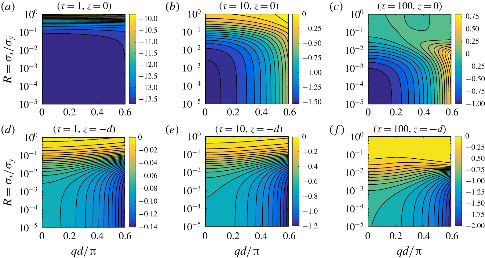
 $\unicode[STIX]{x0394}x$ to be globally zero, which is borne out in figure 4, where we show contour plots of finite-time displacements evaluated by numerical time integration of (3.12). As incompressibility holds, (2.20) indicates that the mass-balance argument is not fundamentally altered by the presence of an internal wave wake in three dimensions. Nor is the fact that the time and area integrals do not commute altered, so that the above again depends on taking the time limit before the limit
 $|y|\rightarrow \infty$, as explained below (2.20).
The special case of a 2-D wavepacket is obtained by setting  $\hat{M}(k,l)=2\unicode[STIX]{x03C0}\hat{M}(k)\unicode[STIX]{x1D6FF}(l)$ in (3.12) and performing the
 $l$-integral. For net displacements, the
 $l$-integral must be performed before the time integral, as discussed in § 2.4 (the integrals over
 $\unicode[STIX]{x1D6FF}(k)$ and
 $\unicode[STIX]{x1D6FF}(l)$ do not commute). This gives
 $|\boldsymbol{k}|\unicode[STIX]{x1D6FD}_{\unicode[STIX]{x1D702},q}(k)=|k/(k+\text{i}\unicode[STIX]{x1D702})|\sqrt{(k+\text{i}\unicode[STIX]{x1D702})^{2}-q^{2}}$, and the velocity integral becomes, following some small-
 $\unicode[STIX]{x1D702}$ approximations,
 $$\begin{eqnarray}\displaystyle u_{2}=-\frac{1}{2\unicode[STIX]{x03C0}}\lim _{\unicode[STIX]{x1D702}\rightarrow 0^{+}}\int _{-\infty }^{\infty }\hat{M}(k)\sqrt{(k+\text{i}\unicode[STIX]{x1D702})^{2}-q^{2}}\frac{\cosh ((z+d)\sqrt{(k+\text{i}\unicode[STIX]{x1D702})^{2}-q^{2}})}{\sinh (d\sqrt{(k+\text{i}\unicode[STIX]{x1D702})^{2}-q^{2}})}\text{e}^{\text{i}k\tilde{x}}\,\text{d}k.\quad & & \displaystyle\end{eqnarray}$$
Integrating over time results in a delta function at  $k=0$, so for a Gaussian packet, the net displacement is then given by
 $$\begin{eqnarray}\displaystyle d^{\ast }\unicode[STIX]{x0394}x^{\ast }(z/d,qd,d^{\ast })=-qd\frac{\cos (qd(1+z/d))}{\sin (qd)}. & & \displaystyle\end{eqnarray}$$
Unlike in the unstratified case, the net displacement is now a function of  $z$ and the parameter
 $qd=Nd/c_{g,0}$, which measures the ratio of ocean depth
 $d$ to the vertical scale (
 $c_{g,0}/N$) of the
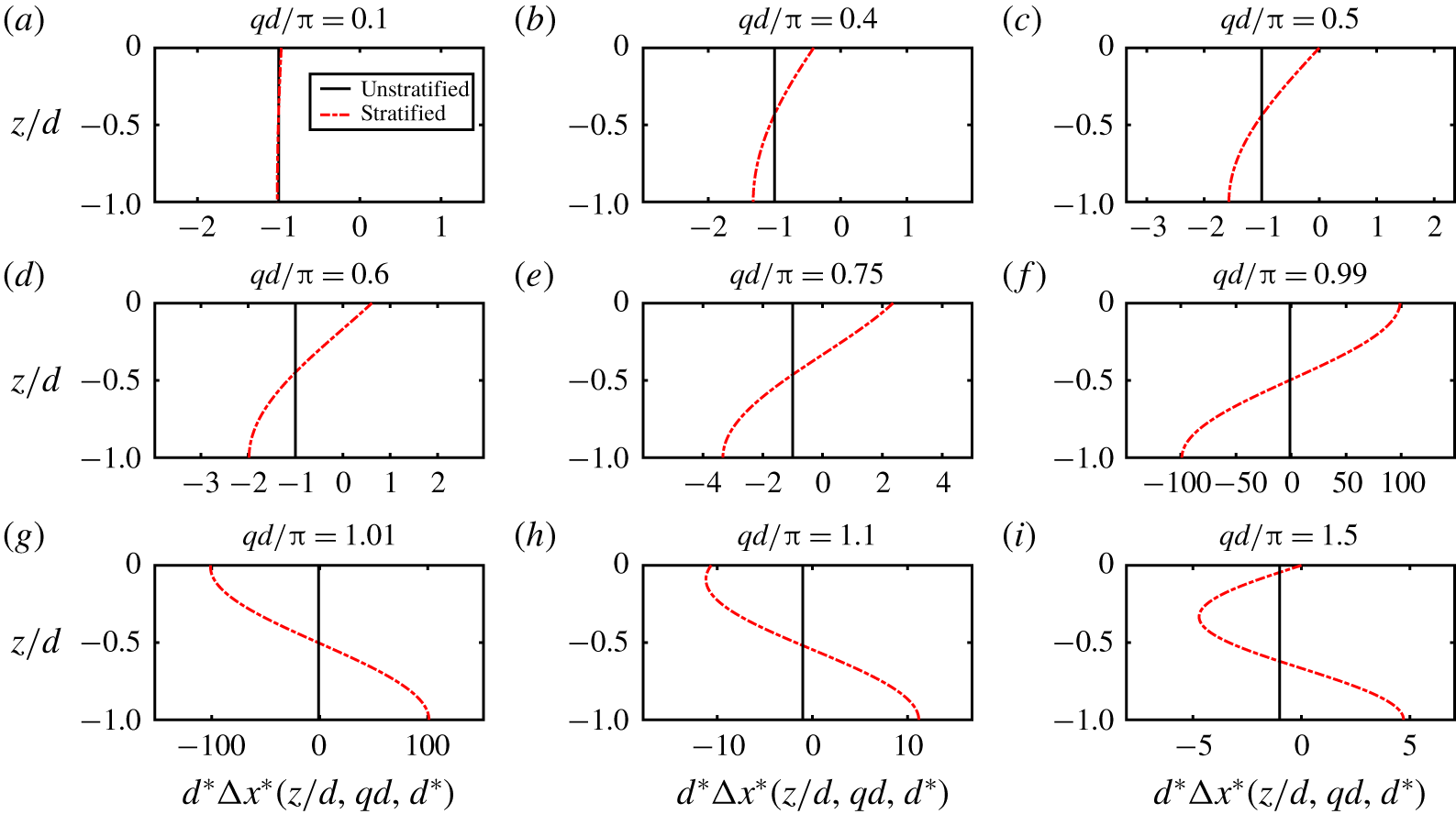
 $k_{1}=\sqrt{q^{2}-\unicode[STIX]{x03C0}^{2}/d^{2}}=0$ internal wave which would be forced were the ocean deep enough. Depth profiles of (3.14) are shown in figure 3 for different
 $qd$-values. We now explore the role of the stratification measure
 $qd$. As
 $qd\rightarrow 0$, a Taylor expansion of (3.14) gives the dependence of net displacement on weak stratification
 $$\begin{eqnarray}\displaystyle \unicode[STIX]{x0394}x^{\ast }=-\frac{1}{d^{\ast }}\left(1+\frac{q^{2}d^{2}}{6}-\frac{q^{2}d^{2}}{2}(1+z/d)^{2}+O((qd)^{3})\right), & & \displaystyle\end{eqnarray}$$
which recovers the unstratified result  $\unicode[STIX]{x0394}x^{\ast }=-1/d^{\ast }$ upon neglecting terms
 $O((qd)^{2})$. To leading order, the magnitude of net displacement is predicted to decrease above a depth
 $z/d=-(1-1/\sqrt{3})\approx -0.42$, and increase below, as shown in figure 3(a,b).
Scaled net displacement  $d^{\ast }\unicode[STIX]{x0394}x^{\ast }$ by the return flow of a 2-D packet in stratified flow from (3.14) as a function of depth
 $z/d$ for various values of the stratification measure
 $qd=Nd/c_{g,0}$.

Contours of scaled finite-time displacement: panels (a–c) correspond to  $z=0$ and (d–f) to
 $z=-d$. Moving from left to right, the half-interval
 $\unicode[STIX]{x1D70F}$ is increased sequentially by a factor of
 $10$, from (a,d) plotted at
 $\unicode[STIX]{x1D70F}=1$, to (c,f) plotted at
 $\unicode[STIX]{x1D70F}=100$.

If  $qd=\unicode[STIX]{x03C0}/2$, the net return-flow displacement remains negative and monotonic throughout the entire depth, but is zero at the surface,
 $$\begin{eqnarray}\displaystyle d^{\ast }\unicode[STIX]{x0394}x^{\ast }=-\frac{\unicode[STIX]{x03C0}}{2}\sin \left(\frac{\unicode[STIX]{x03C0}}{2}\frac{|z|}{d}\right). & & \displaystyle\end{eqnarray}$$
This is illustrated in figure 3(c). The stratification is not yet strong enough to support a wake of internal waves with phase speeds  ${\geqslant}c_{g,0}$, but is sufficiently strong to bring the near-surface displacement to zero. For somewhat greater stratification
 $\unicode[STIX]{x03C0}>qd>\unicode[STIX]{x03C0}/2$, the net displacement becomes positive near the surface, as illustrated in figure 3(d–f).
Only when  $qd>\unicode[STIX]{x03C0}$ are free internal waves generated in the wake of a 2-D packet (figure 3g–i). This corresponds to
 $N>\unicode[STIX]{x03C0}c_{g,0}/d$. As
 $qd$ traverses
 $\unicode[STIX]{x03C0}$ (more generally
 $n\unicode[STIX]{x03C0}$), the displacement profile undergoes a sign change (cf. figure 3f,g). When
 $qd\rightarrow n\unicode[STIX]{x03C0}$, with
 $n$ a positive integer, the displacement becomes singular (and very large in close proximity, cf. figure 3f,g), corresponding to a resonance in which
 $c_{g,0}$ matches the
 $x$-phase speed of a long internal wave with
 $k_{n}=\sqrt{q^{2}-n^{2}\unicode[STIX]{x03C0}^{2}/d^{2}}=0$.
The Stokes drift is unaltered by stratification when the waves are treated as irrotational, so the net Lagrangian displacement in two dimensions is obtained as the expression
 $$\begin{eqnarray}\displaystyle \hspace{-20.0pt}\unicode[STIX]{x0394}x_{L}^{\ast }=\left(2k_{0}\unicode[STIX]{x1D70E}_{x}\text{e}^{2k_{0}z}-\frac{1}{d^{\ast }}(qd)\frac{\cos (qd(1+z/d))}{\sin (qd)}\right). & & \displaystyle\end{eqnarray}$$
The depth integral of (3.17) from  $-d$ to
 $0$ remains zero, so the return flow still balances the transport
 $M$: density stratification alters the manner in which the return flow transports mass without changing the vertically integrated mass balance.
Finally, figure 4 summarises the combined effect of directional spread and stratification by showing contours of scaled finite-time displacement as a function of the stratification measure  $qd/\unicode[STIX]{x03C0}$ and aspect ratio
 $R$ at different
 $\unicode[STIX]{x1D70F}=1,10,100$. To focus on what is realistic for the ocean, we take
 $0\leqslant qd/\unicode[STIX]{x03C0}\leqslant 0.6$ (see table 1), so stratification generally reduces the magnitude of the displacement near the surface and enhances it to become more negative at depth (cf. figure 3a–d). At small
 $\unicode[STIX]{x1D70F}=1$ (figures 4a and 4d), stratification does not have an impact at the surface where the displacements reach their peak values, but its effects can be observed at depth, despite the very small displacements here. At intermediate
 $\unicode[STIX]{x1D70F}\sim 10$ (figures 4b and 4e), negative displacement near the surface is mainly reduced by the influence of spanwise localisation, and only weakly by stratification. The contours at depth resemble those at smaller
 $\unicode[STIX]{x1D70F}\sim 1$ albeit with larger magnitudes, as particles at the bottom begin to experience the flow but have not yet been affected by
 $R$. At large
 $\unicode[STIX]{x1D70F}\sim 100$, displacements have practically vanished for all but very small aspect ratios, recovering the 2-D long-time limit (3.14) as
 $R\rightarrow 0$ (cf. figure 3a–d).
4 Conclusions
We have examined the Lagrangian displacement induced by isolated non-dissipating surface gravity wavepackets and, in particular, the displacement associated with the wave-induced return flow, focussing on the effects of localisation in the spanwise coordinate  $y$ (as a proxy for weak directional spreading) and density stratification. For spanwise-infinite wavepackets (two-dimensional) on an unstratified flow, the net displacement associated with the return flow - where ‘net’ means computed over an infinite time interval as the packet propagates from
 $x=-\infty$ to
 $x=\infty$ – is independent of the depth coordinate
 $z$. The net displacement is inversely proportional to the ocean depth
 $d$, and therefore goes to
 $0$ when
 $d\rightarrow \infty$, as dictated by mass conservation. In the presence of any localisation of the packet in
 $y$, the net displacement becomes zero at each
 $(y,z)$, regardless of the depth
 $d$. Over a finite, symmetric time interval, with the wavepacket starting a finite distance behind the
 $x$-origin and propagating to the same distance ahead (see (2.21)), the return flow in three dimensions initially displaces particles in the same manner as in two dimensions, but ultimately brings particles back to their original positions as the flow returns around as well as underneath the packet. This 2-D–3-D transition occurs on a time scale
 ${\sim}\unicode[STIX]{x1D70E}_{y}/c_{g,0}$, where
 $\unicode[STIX]{x1D70E}_{y}$ is the packet’s width (proportional to the degree of directional spreading) and
 $c_{g,0}$ is the surface wave group velocity.
Density stratification alters the profile of the net displacement by the return flow of 2-D packets: the net displacement becomes an oscillatory function of  $z$ with a wavelength dependent on the parameter
 $qd$, where
 $q\equiv N/c_{g,0}$ is the vertical buoyancy wavenumber,
 $d$ is the ocean depth and
 $N$ is the (constant) buoyancy frequency. For
 $qd<\unicode[STIX]{x03C0}$, as is typical for the ocean, stratification diminishes displacements near the surface and enhances them at depth. When
 $qd\rightarrow \unicode[STIX]{x03C0}$ (more generally, for
 $qd\rightarrow n\unicode[STIX]{x03C0}$), the net displacement becomes singular due to a resonance between
 $c_{g,0}$ and the phase velocity of a long internal wave mode, while for
 $qd>\unicode[STIX]{x03C0}$, it is finite but of opposite sign. In the presence of any localisation of the packet in
 $y$, the net displacement again reduces to zero. Stratification may, however, appreciably alter the finite-time displacement, with the signature of the internal wave wake generally present for all times at depth, and only for larger times at the surface.
In order to obtain a quantitative estimate of magnitudes of the displacements, we recall from (2.15) the displacement scale  $\unicode[STIX]{x1D6FC}^{2}\sqrt{\unicode[STIX]{x03C0}}\unicode[STIX]{x1D70E}_{x}/(k_{0}d)$, with
 $\unicode[STIX]{x1D6FC}\equiv a_{0}k_{0}$, by which we multiply the colour scale in figure 4 to obtain dimensional displacements. To consider how large this displacement scale can be, we take the largest possible value of
 $\unicode[STIX]{x1D6FC}=0.3$, the smallest value of
 $k_{0}d=3$ for the deep-water assumption to still hold, and
 $\unicode[STIX]{x1D70E}_{x}=(2k_{0}\unicode[STIX]{x1D700})^{-1}=3.1\times 10^{2}~\text{m}$, corresponding to typical values
 $\unicode[STIX]{x1D714}_{0}=2\unicode[STIX]{x03C0}/10~\text{s}$,
 $d=75~\text{m}$,
 $\unicode[STIX]{x1D700}=0.04$ (see table 1). We then obtain a displacement scale
 $\unicode[STIX]{x1D6FC}^{2}\sqrt{\unicode[STIX]{x03C0}}\unicode[STIX]{x1D70E}_{x}/(k_{0}d)=17~\text{m}$. For a more usual depth
 $d=3.1\times 10^{3}~\text{m}$, this reduces to
 $0.41~\text{m}$ and even further to
 $0.011~\text{m}$ for the more typical steepness
 $\unicode[STIX]{x1D6FC}=0.05$. For unstratified flow in two dimensions, the displacement scale gives the dimensional net return-flow displacement (times
 $-1$). We will now consider typical values of
 $qd$ and
 $R=\unicode[STIX]{x1D70E}_{x}/\unicode[STIX]{x1D70E}_{y}$.
Realistic parameter ranges and typical values chosen (compiled from Ewans (Reference Ewans2002), van den Bremer & Taylor (Reference van den Bremer and Taylor2015), Haney & Young (Reference Haney and Young2017) and Toffoli & Bitner-Gregersen (Reference Toffoli and Bitner-Gregersen2017)).

4.1 Quantitative effect of directional spreading
In order to relate the value of the packet aspect ratio  $R$ to typical values of the (root-mean-square) directional spreading of the energy spectrum
 $\unicode[STIX]{x1D70E}_{\unicode[STIX]{x1D703}}$ reported in the literature (e.g. Ewans Reference Ewans2002), we use the relationship
 $R\approx \sqrt{2}\unicode[STIX]{x1D700}\unicode[STIX]{x1D70E}_{\unicode[STIX]{x1D703}}$, which is only valid in the limit of weak directional spreading. Taking a value of
 $\unicode[STIX]{x1D70E}_{\unicode[STIX]{x1D703}}=5.0^{\circ }$ typical of swell conditions (Ewans Reference Ewans2002) and
 $\unicode[STIX]{x1D700}=0.04$, we obtain
 $R=4.9\times 10^{-3}$, increasing to
 $R=1.9\times 10^{-2}$ for a very narrow-banded packet with
 $\unicode[STIX]{x1D700}=0.15$, and further to
 $R=0.11$ for a highly directionally spread packet with
 $\unicode[STIX]{x1D70E}_{\unicode[STIX]{x1D703}}=30^{\circ }$. The time scale on which the transition from 2-D-like to 3-D-like behaviour occurs
 ${\sim}\unicode[STIX]{x1D70E}_{x}/(c_{g,0}R)=(R\unicode[STIX]{x1D700}\unicode[STIX]{x1D714}_{0})^{-1}$, can thus be as large as
 $8.1\times 10^{3}~\text{s}$ (
 $R=4.9\times 10^{-3},\unicode[STIX]{x1D700}=0.04$) or
 $3.6\times 10^{2}~\text{s}$ (
 $R=0.11,\unicode[STIX]{x1D700}=0.15$) for the typical
 $\unicode[STIX]{x1D714}_{0}=2\unicode[STIX]{x03C0}/10~\text{s}^{-1}$ considered before, with corresponding much shorter packet-translation times of
 $\unicode[STIX]{x1D70E}_{x}/c_{g,0}\approx 40~\text{s}$ and
 $11~\text{s}$, respectively.
4.2 Quantitative effect of stratification
Taking a typical ocean depth  $d=3.1\times 10^{3}~\text{m}$ and a (constant) value of
 $N=2\unicode[STIX]{x03C0}/1333~\text{s}^{-1}$, we obtain
 $qd/\unicode[STIX]{x03C0}=0.6$. The 2-D net return-flow displacement is then zero at
 $z=-5.0\times 10^{2}~\text{m}$ (cf. figure 3d). Net displacement at the surface is positive, and its maximum (negative) value occurs at the ocean floor. The behaviour predicted for larger
 $qd$ values, including the resonance at
 $qd=n\unicode[STIX]{x03C0}$, is unlikely to arise in the real ocean, since stratification is generally too weak to satisfy this resonance. Furthermore, the depth variability of
 $N$ observed in real oceans (e.g. exponential, or piecewise linear in a crude approximation) would likely weaken the role of stratification predicted here, and prevent exact resonances. Large displacements are also likely to be mitigated by viscous dissipation, and we expect that, near resonance, transfer of energy from the surface wavepacket to the internal wave wake may lead to disintegration of the packet.
4.3 Neglected effects: wave dispersion, viscosity and the Earth’s rotation
In this paper, in addition to considering the abstract case of an isolated wavepacket, we have ignored the effects of wave dispersion beyond leading order in  $\unicode[STIX]{x1D700}$, viscosity (resulting in a non-dissipating wavepacket) and the Earth’s rotation. We will explore the potential consequences of these assumptions below. In terms of wave dispersion, we have examined only leading-order solutions in the small bandwidth parameter
 $\unicode[STIX]{x1D700}$; at the next order, two effects need to be accounted for. First, we used the rigid-lid approximation to neglect the set-down of the wave-averaged free surface
 $h_{2}$ (given by (2.5)) when calculating return-flow displacements. In appendix A, we show that including the set-down results in multiplication of the net displacement by at most a factor
 $(1-\unicode[STIX]{x1D700}^{2}\unicode[STIX]{x1D70E}_{x}/d)^{-1}$, with the largest correction occurring for a 2D shallow return flow. Even for larger
 $\unicode[STIX]{x1D700}$, this effect is small. Second, we have assumed that the packet propagates without any change in shape. In appendix B we find that, to leading order, the enhancement of displacement due to wave dispersion is
 $(1+\unicode[STIX]{x1D700}^{2}/2)$, which again is small even for large
 $\unicode[STIX]{x1D700}$.
Longuet-Higgins (Reference Longuet-Higgins1953) introduced viscous boundary layers, of the type studied by Rayleigh (Reference Rayleigh1883), in which mean vorticity is generated and then slowly diffused into the fluid interior, eventually altering the mass transport profiles. The viscous boundary layer thickness  $\unicode[STIX]{x1D6FF}=\sqrt{2\unicode[STIX]{x1D708}/\unicode[STIX]{x1D714}_{0}}$, where
 $\unicode[STIX]{x1D708}$ is the kinematic viscosity of seawater, is generally of the order of millimetres. When
 $a_{0}^{2}\gg \unicode[STIX]{x1D6FF}^{2}$, the relevant case for a wavepacket, vorticity diffuses into the fluid interior on a time scale
 ${\sim}\unicode[STIX]{x1D70E}_{x}/(a^{2}\unicode[STIX]{x1D714}k)=\unicode[STIX]{x1D6FC}^{-2}\unicode[STIX]{x1D700}^{-1}\unicode[STIX]{x1D714}_{0}^{-1}$. This process takes multiple packet-translation times, so vorticity will not have had sufficient time to diffuse into the fluid interior before the packet has propagated past. Nevertheless, the long-time behaviour may be affected.
On a rotating earth, Ursell (Reference Ursell1950) demonstrated that a steady Stokes drift would violate conservation of circulation, implying that the Lagrangian-mean velocity accompanying a regular, horizontally uniform wavetrain must be zero in the long-time average over many inertial periods. It follows that there must be a long-time-average Eulerian-mean ‘anti-Stokes flow’ possessing vorticity, cancelling the Stokes drift. In an initial-value problem starting with an irrotational Stokes wave with its Stokes drift – as with swell arriving in previously calm water – the Coriolis force induces free inertial oscillations. Further aspects of this problem were explored in Hasselmann (Reference Hasselmann1970). As periods associated with the Earth’s rotation are much longer than the translation time scale of a narrow-banded packet (see also Herbers & Janssen (Reference Herbers and Janssen2016)), we anticipate that Coriolis effects can be neglected when considering net displacements by the return flow. Two dimensionless numbers may play a role:  $f\unicode[STIX]{x1D70E}_{x}/c_{g,0}$ and
 $f\unicode[STIX]{x1D70E}_{y}/c_{g,0}$. The first (
 $f\unicode[STIX]{x1D70E}_{x}/c_{g,0}$) is only appreciably large for a long, slow-moving packet, or for strong rotation. However, the second is large for almost-unidirectional waves, leaving open the possibility that rotation affects the mean flow, which we hope to examine in future work. We also note that, when rotation and eddy viscosity are included together, the mean flow may be appreciably changed over the associated Ekman depth
 ${\sim}(2\unicode[STIX]{x1D708}/f)^{1/2}$, which in real oceans is comparable to the Stokes depth
 ${\sim}(2k_{0})^{-1}$ (e.g. Xu & Bowen Reference Xu and Bowen1994). We do not consider these effects herein.
Acknowledgements
The authors thank two anonymous referees for many useful comments which have improved our paper.
Appendix A. Inclusion of the set-down
In this appendix, we consider how the set-down of the wave-averaged free surface,  $h_{2}$, affects the net displacement by a 2-D return flow. We have previously used the rigid-lid approximation to neglect the set-down (given by (2.5)), which corresponds to ignoring
 $\unicode[STIX]{x2202}_{t}^{2}\unicode[STIX]{x1D719}_{2}$ on the left-hand side of (2.4) when calculating the return-flow potential. Up to
 $O(\unicode[STIX]{x1D6FC}^{2}\unicode[STIX]{x1D700}^{3})$ the overbarred term in (2.4) is zero and the Stokes transport
 $M$ remains unchanged, so only the linear operator acting on
 $\unicode[STIX]{x1D719}_{2}$ is altered by including the set-down,
 $$\begin{eqnarray}\displaystyle \left.\left(\frac{c_{g,0}^{2}}{g}\unicode[STIX]{x2202}_{\tilde{x}}^{2}+\unicode[STIX]{x2202}_{z}\right)\unicode[STIX]{x1D719}_{2}\right|_{z=0}=\unicode[STIX]{x2202}_{\tilde{x}}M, & & \displaystyle\end{eqnarray}$$
where we have moved into the group frame  $\tilde{x}\equiv (x-c_{g,0}t)$. The solution to the Laplace equation which obeys (A 1) and a no-flow bottom boundary is
 $$\begin{eqnarray}\unicode[STIX]{x1D719}_{2}=\frac{\unicode[STIX]{x1D714}_{0}a_{0}^{2}\unicode[STIX]{x1D70E}_{x}\unicode[STIX]{x1D70E}_{y}}{8\unicode[STIX]{x03C0}}\iint _{\mathbb{R}^{2}}\frac{\text{i}k\text{e}^{-k^{2}\unicode[STIX]{x1D70E}_{x}^{2}/4-l^{2}\unicode[STIX]{x1D70E}_{y}^{2}/4}}{\sqrt{k^{2}+l^{2}}-{\displaystyle \frac{\unicode[STIX]{x1D700}c_{g,0}^{2}k^{2}}{g\tanh (d\sqrt{k^{2}+l^{2}})}}}\frac{\cosh ((z+d)\sqrt{k^{2}+l^{2}})}{\sinh (d\sqrt{k^{2}+l^{2}})}\text{e}^{\text{i}k\tilde{x}}\text{e}^{\text{i}ly}\,\text{d}k\,\text{d}l.\end{eqnarray}$$
This is similar to (2.16), but the denominator is now modified due to the set-down term; since  $k^{2}/\tanh (d\sqrt{k^{2}+l^{2}})$ is always positive, the set-down enhances the return flow. As we have shown that the net displacement disappears in three dimensions (see (2.17)) but behaves two-dimensionally for short times (see § 2.4,
 $t_{\mathit{I}}<\unicode[STIX]{x1D70E}_{y}/c_{g,0}$), we will only consider the 2-D displacement here. The horizontal velocity in two dimensions is given by
 $$\begin{eqnarray}\displaystyle u_{2}=-\frac{\unicode[STIX]{x1D714}a_{0}^{2}\unicode[STIX]{x1D70E}_{x}}{4\sqrt{\unicode[STIX]{x03C0}}}\int _{-\infty }^{\infty }\frac{k\text{e}^{-k^{2}\unicode[STIX]{x1D70E}_{x}^{2}/4}}{1-{\displaystyle \frac{\unicode[STIX]{x1D700}c_{g,0}^{2}k}{g\tanh (kd)}}}\frac{\cosh (k(z+d))}{\sinh (kd)}\text{e}^{\text{i}k\tilde{x}}\,\text{d}k. & & \displaystyle\end{eqnarray}$$
Integrating over all time (all  $\tilde{x}/c_{g,0}$ in the co-moving packet frame) results in a delta function at
 $k=0$, so the net displacement (dimensional and scaled respectively) is
 $$\begin{eqnarray}\displaystyle \unicode[STIX]{x0394}x=-\frac{\unicode[STIX]{x1D714}_{0}a_{0}^{2}\sqrt{\unicode[STIX]{x03C0}}}{2c_{g,0}}\frac{\unicode[STIX]{x1D70E}_{x}}{d}\frac{1}{(1-\unicode[STIX]{x1D700}c_{g,0}^{2}/(gd))},\quad \unicode[STIX]{x0394}x^{\ast }=-\frac{1}{d^{\ast }}\frac{1}{(1-\unicode[STIX]{x1D700}^{2}/(2d^{\ast }))}, & & \displaystyle\end{eqnarray}$$
with  $d^{\ast }\equiv d/\unicode[STIX]{x1D70E}_{x}$ the ocean depth scale with respect to the packet length. Inclusion of the set-down in two dimensions therefore results in multiplication of the net displacement by
 $(1-\unicode[STIX]{x1D700}c_{g,0}^{2}/gd)^{-1}$, which may alternatively be written as
 $(1-\unicode[STIX]{x1D700}^{2}/(2d^{\ast }))$ using the definition
 $\unicode[STIX]{x1D700}\equiv (2k_{0}\unicode[STIX]{x1D70E}_{x})^{-1}$. Hence, when
 $k_{0}d\gg 1$ and
 $\unicode[STIX]{x1D700}\ll 1$ such that
 $d^{\ast }=2\unicode[STIX]{x1D700}(k_{0}d)\gg 1$, it is justified to make the rigid-lid approximation by neglecting
 $\unicode[STIX]{x2202}_{t}h_{2}$ in (2.1b) when calculating the leading-order return flow in deep water. We note from (A 4b) that the effect of the set-down is largest when the return flow is two-dimensional (
 $R=0$) and shallow (
 $d^{\ast }\equiv d/\unicode[STIX]{x1D70E}_{x}\ll 1$); for a large bandwidth
 $\unicode[STIX]{x1D700}=0.125$ and a depth scale
 $d^{\ast }=1/2$, the correction is approximately
 $3\,\%$.
Appendix B. The leading-order effect of wave dispersion
In this appendix, we explore the effect of wave dispersion on the net Lagrangian displacement in unstratified flow, over times  $t$ satisfying
 $\unicode[STIX]{x1D700}^{2}t=O(1)$. To do so, we update the linear quantities (2.2) to include dependence on a slow time scale
 $T=\unicode[STIX]{x1D700}^{2}t$ in § B.1 (see also e.g. Kinsman (Reference Kinsman2002)), and in § B.2 we determine the mean-flow forcing (2.4) at
 $O(\unicode[STIX]{x1D6FC}^{2}\unicode[STIX]{x1D700}^{2})$ accordingly, examining the full 3-D case.
B.1 First-order solutions $O(\unicode[STIX]{x1D6FC})$

From the combined linear boundary condition  $(\unicode[STIX]{x2202}_{t}^{2}+g\unicode[STIX]{x2202}_{z})\unicode[STIX]{x1D719}_{1}|_{z=0}=0$, we obtain an evolution equation for
 $A_{0}$ in terms of the
 $O(\unicode[STIX]{x1D700}^{2})$ time scale and its Fourier-space solution,
 $$\begin{eqnarray}\displaystyle \unicode[STIX]{x2202}_{T}A_{0}=\text{i}\frac{c_{g,0}^{2}}{2\unicode[STIX]{x1D714}_{0}}\unicode[STIX]{x2202}_{\tilde{x}\tilde{x}}A_{0},\quad \hat{A}_{0}(k,l,T)=\hat{A}_{0}(k,l)\text{e}^{\text{i}k^{2}\unicode[STIX]{x1D6FE}_{0}T/2}, & & \displaystyle\end{eqnarray}$$
where  $\unicode[STIX]{x1D6FE}_{0}\equiv \unicode[STIX]{x2202}^{2}\unicode[STIX]{x1D714}_{0}/\unicode[STIX]{x2202}k_{0}^{2}=-\sqrt{g/k_{0}^{3}}/4$ is the dispersive parameter. Assuming the surface profile is Gaussian, inverting the transform (B 1b) shows that the surface maintains its Gaussian shape, but now evolves on the slow, dispersive time scale,
 $$\begin{eqnarray}\displaystyle A_{0}(x,y,T)=a_{0}^{Disp}\text{e}^{-\tilde{x}^{2}/(2(\unicode[STIX]{x1D70E}_{x}^{Disp})^{2})}\text{e}^{-y^{2}/(2\unicode[STIX]{x1D70E}_{y}^{2})}, & & \displaystyle\end{eqnarray}$$
where the ‘ $\text{Disp}$’ superscript denotes inclusion of leading-order dispersion, and slowly varying parameters are
 $$\begin{eqnarray}\displaystyle a_{0}^{Disp}=\frac{a_{0}}{\sqrt[4]{1+\unicode[STIX]{x1D6FE}_{0}^{2}t^{2}/\unicode[STIX]{x1D70E}_{x}^{4}}},\quad \unicode[STIX]{x1D70E}_{x}^{Disp}=\unicode[STIX]{x1D70E}_{x}\sqrt{1+\unicode[STIX]{x1D6FE}_{0}^{2}t^{2}/\unicode[STIX]{x1D70E}_{x}^{4}}. & & \displaystyle\end{eqnarray}$$
Dispersion is hence important for times  ${\gtrsim}\unicode[STIX]{x1D70E}_{x}^{2}/|\unicode[STIX]{x1D6FE}_{0}|$. Over time, the packet decreases in amplitude and widens as it translates at the group velocity
 $c_{g,0}$. It is therefore no longer steady in its own reference frame.
B.2 Second-order solutions $O(\unicode[STIX]{x1D6FC}^{2})$

From appendix A the set-down contribution is  $O(\unicode[STIX]{x1D700}^{2}/d^{\ast })$, so we include the
 $\unicode[STIX]{x2202}_{t}^{2}$ term on the left-hand side of (2.4), whilst emphasising that this term is due to the set-down rather than wave dispersion. It is found that
 $O(\unicode[STIX]{x1D6FC}^{1}\unicode[STIX]{x1D700}^{1})$ terms in (2.2a), (2.2b) do not contribute to the right-hand side of (2.4) at
 $O(\unicode[STIX]{x1D6FC}^{2}\unicode[STIX]{x1D700}^{2})$; the wave forcing obtained by multiplying
 $O(\unicode[STIX]{x1D6FC}^{1}\unicode[STIX]{x1D700}^{1})$ terms by
 $O(\unicode[STIX]{x1D6FC}^{1}\unicode[STIX]{x1D700}^{0})$ terms in (2.2) disappears under wave averaging. Consequently, we need only account for functional dependence of
 $A_{0}$ (see (B 1)) on
 $T=\unicode[STIX]{x1D700}^{2}t=O(1)$ to calculate the updated
 $M$. At
 $O(\unicode[STIX]{x1D6FC}^{2}\unicode[STIX]{x1D700}^{2})$, the mean flow is still forced solely by the Stokes transport, which is now slowly evolving. The boundary condition for
 $\unicode[STIX]{x1D719}_{2}$ is
 $$\begin{eqnarray}\displaystyle \left.\left(\frac{c_{g,0}^{2}}{g}\unicode[STIX]{x2202}_{\tilde{x}}^{2}+\unicode[STIX]{x2202}_{z}\right)\unicode[STIX]{x1D719}_{2}^{Disp}\right|_{z=0}=\unicode[STIX]{x2202}_{\tilde{x}}M^{Disp}. & & \displaystyle\end{eqnarray}$$
Solving (B 4) in Fourier space, we obtain
 $$\begin{eqnarray}\displaystyle \unicode[STIX]{x1D719}_{2}^{Disp} & = & \displaystyle \frac{\unicode[STIX]{x1D714}_{0}|a_{0}^{Disp}|^{2}\unicode[STIX]{x1D70E}_{x}^{Disp}\unicode[STIX]{x1D70E}_{y}}{8\unicode[STIX]{x03C0}}\iint _{\mathbb{R}^{2}}\frac{\text{i}k\text{e}^{-k^{2}(\unicode[STIX]{x1D70E}_{x}^{Disp})^{2}/4-l^{2}\unicode[STIX]{x1D70E}_{y}^{2}/4}}{\sqrt{k^{2}+l^{2}}-{\displaystyle \frac{\unicode[STIX]{x1D700}c_{g,0}^{2}k^{2}}{g\tanh (d\sqrt{k^{2}+l^{2}})}}}\nonumber\\ \displaystyle & & \displaystyle \times \,\frac{\cosh ((z+d)\sqrt{k^{2}+l^{2}})}{\sinh (d\sqrt{k^{2}+l^{2}})}\text{e}^{\text{i}k\tilde{x}}\text{e}^{\text{i}ly}\,\text{d}k\,\text{d}l.\end{eqnarray}$$
The finite-time 3-D return-flow displacement is expressed as the triple integral (with  $\hat{t}=c_{g,0}t/\unicode[STIX]{x1D70E}_{x}$ dimensionless packet time,
 $\unicode[STIX]{x1D705}=k\unicode[STIX]{x1D70E}_{x}$ and
 $\unicode[STIX]{x1D706}=l\unicode[STIX]{x1D70E}_{y}$),
 $$\begin{eqnarray}\displaystyle \unicode[STIX]{x0394}x^{\ast ,Disp}(\unicode[STIX]{x1D70F},R,z^{\ast }) & = & \displaystyle -\frac{1}{2\unicode[STIX]{x03C0}^{3/2}}\iint _{\mathbb{R}^{2}}\int _{0}^{\unicode[STIX]{x1D70F}}\frac{\unicode[STIX]{x1D705}^{2}\text{e}^{-\unicode[STIX]{x1D706}^{2}/4}\text{e}^{-\unicode[STIX]{x1D705}^{2}(1+\unicode[STIX]{x1D700}^{2}\hat{t}^{2})/4}}{\sqrt{\unicode[STIX]{x1D705}^{2}+R^{2}\unicode[STIX]{x1D706}^{2}}-{\displaystyle \frac{\unicode[STIX]{x1D700}^{2}\unicode[STIX]{x1D705}^{2}}{\tanh (d^{\ast }\sqrt{\unicode[STIX]{x1D705}^{2}+R^{2}\unicode[STIX]{x1D706}^{2}})}}}\cos (\unicode[STIX]{x1D705}\hat{t})\nonumber\\ \displaystyle & & \displaystyle \times \,\frac{\cosh ((z^{\ast }+d^{\ast })\sqrt{\unicode[STIX]{x1D705}^{2}+R^{2}\unicode[STIX]{x1D706}^{2}})}{\sinh (d^{\ast }\sqrt{\unicode[STIX]{x1D705}^{2}+R^{2}\unicode[STIX]{x1D706}^{2}})}\,\text{d}\unicode[STIX]{x1D705}\,\text{d}\unicode[STIX]{x1D706}\,\text{d}\hat{t}.\end{eqnarray}$$
Using complex exponentials, we can first exactly evaluate the finite-time integral
 $$\begin{eqnarray}\displaystyle \int _{0}^{\unicode[STIX]{x1D70F}}\text{e}^{-\unicode[STIX]{x1D700}^{2}\unicode[STIX]{x1D705}^{2}\hat{t}^{2}/4}\cos (\unicode[STIX]{x1D705}\hat{t})\,\text{d}\hat{t}=\frac{\sqrt{\unicode[STIX]{x03C0}}}{2\unicode[STIX]{x1D705}}\frac{\text{e}^{-\frac{1}{\unicode[STIX]{x1D700}^{2}}}}{\unicode[STIX]{x1D700}}\text{Re}\left\{\text{erf}\left(\frac{\unicode[STIX]{x1D700}\unicode[STIX]{x1D705}\unicode[STIX]{x1D70F}}{2}+\frac{\text{i}}{\unicode[STIX]{x1D700}}\right)\right\}. & & \displaystyle\end{eqnarray}$$
In the long-time limit, (B 7) is dominated by its behaviour near  $\unicode[STIX]{x1D705}=0$ (e.g. the delta-function result (2.17)), and so over long times we must expand the error function for
 $\unicode[STIX]{x1D700}\unicode[STIX]{x1D705}\unicode[STIX]{x1D70F}\ll 1/\unicode[STIX]{x1D700}$ when
 $\unicode[STIX]{x1D70F}\gg 1$. Taking
 $\exp (-\unicode[STIX]{x1D700}^{2}\unicode[STIX]{x1D705}^{2}\unicode[STIX]{x1D70F}^{2}/4)\approx 1$, the dispersive correction is
 $O(\unicode[STIX]{x1D700}^{2})$,
 $$\begin{eqnarray}\displaystyle \frac{\sqrt{\unicode[STIX]{x03C0}}\text{e}^{-\frac{1}{\unicode[STIX]{x1D700}^{2}}}}{2\unicode[STIX]{x1D700}}\text{Re}\left\{\frac{1}{\unicode[STIX]{x1D705}}\text{erf}\left(\frac{\unicode[STIX]{x1D700}\unicode[STIX]{x1D705}\unicode[STIX]{x1D70F}}{2}+\frac{\text{i}}{\unicode[STIX]{x1D700}}\right)\right\}=\frac{\sin (\unicode[STIX]{x1D705}\unicode[STIX]{x1D70F})}{\unicode[STIX]{x1D705}}\left(1+\frac{\unicode[STIX]{x1D700}^{2}}{2}+O(\unicode[STIX]{x1D700}^{4})\right). & & \displaystyle\end{eqnarray}$$
The delta function result implies the condition  $\unicode[STIX]{x1D700}\unicode[STIX]{x1D705}\unicode[STIX]{x1D70F}\ll 1/\unicode[STIX]{x1D700}$, which suggests we must expand the error function as in (B 8) to be consistent with the separation of scales. While the net displacement remains zero in three dimensions (
 $\sin (\unicode[STIX]{x1D705}\unicode[STIX]{x1D70F})/\unicode[STIX]{x1D705}\rightarrow \unicode[STIX]{x03C0}\unicode[STIX]{x1D6FF}(\unicode[STIX]{x1D705})$ as
 $\unicode[STIX]{x1D70F}\rightarrow \infty$), dispersion weakly enhances the finite-time displacement.