

1. Introduction
An analytic L-function is a Dirichlet series that converges absolutely in some right half plane, has a meromorphic continuation to a function of order 1 with finitely many poles, satisfies a functional equation, and admits an Euler product. For example, the (incomplete) L-functions attached to tempered, cuspidal automorphic representations, or the Hasse–Weil L-functions attached to non-singular, projective, algebraic varieties defined over a number field, conjecturally satisfy these conditions.
In this paper, using standard techniques from analytic number theory, we prove a strong multiplicity one result for such L-functions, without reference to any underlying automorphic or geometric object. We closely follow the work of Kaczorowski and Perelli [ Reference Kaczorowski and Perelli23 ] but redo their arguments for two reasons. First, our results are more general in that they have slightly weaker hypotheses. Second, we think that the techniques should be better known, especially to those who study L-functions automorphically. In the spirit of this second motivation, we offer a series of intuitions about the analytic properties of L-functions that allow us to prove our theorems.
The multiplicity one results we discuss in this paper are statements which assert that if two L-functions are sufficiently close, then they must be equal. A model example is:
Theorem 1·1. Suppose
 $L_1(s)=\sum a_nn^{-s}$
and
 $L_2(s)=\sum b_nn^{-s}$
are Dirichlet series which continue to meromorphic functions of order 1 satisfying appropriate functional equations and having appropriate Euler products. Assume that
 $L_1(s)$
and
 $L_2(s)$
satisfy the Ramanujan conjecture. Assume also that
 $a_p=b_p$
for almost all p. Then
 $L_1(s)=L_2(s)$
.
The precise conditions on the functional equation and Euler product are described in Section 2·1. A weaker version of Theorem 1·1, requiring equality of the local Euler factors instead of the pth Dirichlet coefficients, is given in [ Reference Rudnick and Sarnak40 ]. Theorem 1·1 is also a consequence of the main result in [ Reference Kaczorowski and Perelli23 ]. The result we will actually prove, Theorem 2·3, is stronger. First, instead of requiring equality of the pth Dirichlet series coefficients, we only require that they are close on average. Second, the Ramanujan hypothesis can be slightly relaxed.
We will present some applications of strong multiplicity one for L-functions. The first application is to cuspidal automorphic representations of
 $\textrm{GL}(n,\mathbb{A}_\mathbb{Q})$
, where
 $\mathbb{A}_\mathbb{Q}$
denotes the ring of adeles of the number field
 $\mathbb{Q}$
. Any such representation
 $\pi$
factors as
 $\pi=\otimes\pi_p$
, where
 $\pi_p$
is an irreducible admissible representation of
 $\textrm{GL}(n,\mathbb{Q}_p)$
(we mean
 $\mathbb{Q}_p=\mathbb{R}$
for
 $p=\infty$
). Attached to
 $\pi$
is an automorphic L-function
 $L(s,\pi)$
, whose finite part is
 $L_{\textrm{fin}}(s,\pi) = \prod_{p \lt \infty} L(s, \pi_p)$
. The completion of
 $L_{\textrm{ fin}}(s,\pi)$
is known to be “nice”, and hence
 $L_{\textrm{fin}}(s,\pi)$
is the kind of function to which Theorem 1·1 applies. At almost all primes p we have
 $L(s,\pi_p)=\det(1-A(\pi_p)p^{-s})^{-1}$
, where
 $A(\pi_p)=\textrm{diag}(\alpha_{1,p},\ldots,\alpha_{n,p})$
is a diagonal matrix whose entries are the Satake parameters at p. The Ramanujan conjecture is the assertion that each
 $\pi_p$
is tempered, which in this context implies that
 $|\alpha_{j,p}|=1$
. In particular note that
 $L(s,\pi_p)$
is a polynomial in
 $p^{-s}$
and this polynomial has all its roots on the unit circle.
An easy consequence of Theorem 1·1 is the following.
Theorem 1·2. Suppose that
 $\pi$
and
 $\pi'$
are (unitary) cuspidal automorphic representations of
 $\textrm{GL}(n,\mathbb{A}_\mathbb{Q})$
satisfying
 $\mathrm{tr}(A(\pi_p))=\mathrm{tr}(A(\pi_p'))$
for almost all p. Assume that both
 $L_{\textrm{fin}}(s,\pi)$
and
 $L_{\textrm{ fin}}(s,\pi')$
satisfy the Ramanujan conjecture. Then
 $\pi=\pi'$
.
Most statements of strong multiplicity one in the literature are phrased in terms of
 $A(\pi_p)$
and
 $A(\pi_p')$
being conjugate, instead of the much weaker condition of the equality of their traces. Using the stronger version of Theorem 1·1, we will in fact prove a stronger result which only requires that the traces are close enough on average; see Corollary 3·2 for the precise statement.
Our second application is to paramodular forms of degree 2. For such modular forms Weissauer [
Reference Weissauer49
] has proved the Ramanujan conjecture. The Dirichlet coefficients
 $a_p, b_p$
appearing in Theorem 1·1 are essentially the Hecke eigenvalues for the Hecke operator T(p). We therefore have the following:
Theorem 1·3. Suppose
 $F_j$
, for
 $j=1,2$
, are Siegel paramodular eigenforms of weight
 $k_j$
for the paramodular group of level
 $N_j$
, with Hecke eigenvalues
 $\mu_j(n)$
. Suppose, too, that the
 $F_i$
are not Saito-Kurokawa lifts. If
 $p^{3/2-k_1}\mu_1(p)=p^{3/2-k_2}\mu_2(p)$
for all but finitely many p, then
 $k_1 = k_2$
,
 $N_1=N_2$
and
 $F_1, F_2$
have the same eigenvalues for the Hecke operator T(n) for all n. Furthermore,
 $F_1$
is a scalar multiple of
 $F_2$
.
The remarkable fact here is that the Hecke operator T(p) alone does not generate the local Hecke algebra at p. This Hecke algebra is generated by T(p) and
 $T(p^2)$
. The fact that the coincidence of the eigenvalues for T(p) is enough is of course a global phenomenon. Using the results of [
Reference Schmidt43
], we get the conclusion that
 $F_1$
is a multiple of
 $F_2$
. Again, using the version in Theorem 2·3, we can prove a stronger result; see Theorem 4·2.
We conclude the paper with a discussion of the relative merits of the two types of multiplicity one theorems for L-functions: those which only make use of the L-function axioms, and those which make use of the underlying objects associated to an L-function.
1·1. Analytic vs. automorphic L-functions
The results we present in this paper primarily consider L-functions defined axiomatically: Dirichlet series with a functional equation and an Euler product, having an analytic continuation that satisfies a functional equation. We will refer to these as “analytic” L-functions.
All known analytic L-functions are (in some cases conjecturally) the L-function of an arithmetic object. The existence of such underlying objects may make it possible to prove stronger multiplicity one results for the L-functions. For example, for L-functions of cuspidal automorphic representations on
 $\textrm{GL}(n)$
, there are results much stronger than what follows from our main result. See Section 3. Combining this with Arthur’s lift from
 $\textrm{Sp}(4)$
to
 $\textrm{GL}(4)$
would give a stronger version of the multiplicity one results we have given for Siegel modular forms; see Theorem 4·2.
There are examples of L-functions which have not been proven to be automorphic, such as certain symmetric power L-functions. In such a case, the only option is to use an analytic multiplicity one result, such as those we prove in this paper.
1·2. Comparison with other analytic multiplicity one results
We briefly compare our result to other “analytic” strong multiplicity one results due to Murty and Murty [
Reference Murty and Murty31
], Murty [
Reference Murty30
], Kaczorowski and Perelli [
Reference Kaczorowski and Perelli23
] and Kaczorowski [
Reference Kaczorowski22
]. Roughly speaking, these earlier versions of strong multiplicity one place more and more conditions on the two L-function. In [
Reference Murty and Murty31
], one can find the hypothesis that
 $a_p=b_p$
and
 $a_{p^2}=b_{p^2}$
, in [
Reference Murty30
] it is assumed that
 $a_p=b_p$
and some conditions on the twists of the L-functions. Later, in [
Reference Kaczorowski and Perelli23
], the conditions on the twists of the L-functions is replaced with the assumption that the L-functions have Euler products of a form similar to what we assume. Also relevant are the multiplicity one theorems of Soundararajan [
Reference Soundararajan48
] and M. Farmer [
Reference Farmer17
], which are stated in the most general case of the Selberg class.
We highlight a few notable differences between these earlier versions of strong multiplicity one and ours, making a more thorough comparison between the version by Kaczorowski [
Reference Kaczorowski22
] as it is the most recent and is closest to our version. First, in [
Reference Kaczorowski22
] it is assumed that the L-functions satisfy the Ramanujan bound while we only assume a partial Ramanujan bound. Second, [
Reference Kaczorowski22
] requires the coefficients to be close in the sense
 $|a_p-b_p|\ll p^{-\frac12 -\delta}$
for some
 $\delta\gt0$
, while we allow
 $\delta=0$
. In the proof, our result requires an analysis of possible zeros on the
 $\sigma= 1/2$
-line, while this is avoided if
 $\delta\gt0$
. Finally, the main corollaries of our result do not follow if one requires
 $\delta\gt0$
. Despite these differences, the method of proof is similar, being closely based on [
Reference Kaczorowski and Perelli23
].
The most salient difference between this paper and the papers with the earlier versions of strong multiplicity one is that we have applications in mind. The consequences we prove are of broad interest and lie in different areas of number theory. We include the proofs of the analytic results for completeness and to expose these techniques to as broad an audience as possible.
Notation
We review some notation from analytic number theory. Given two functions
 $f(x),\,g(x)$
, we write:
-
(i)
 $f(x)\sim g(x)$
as
$x\to\infty$
if
$\lim_{x\to\infty} f(x)/g(x)=1$
;
-
(ii)
$f(x) \ll g(x)$
as
$x \to \infty$
if there exists
$C\gt0$
and
$x_0\gt0$
so that if
$x \gt x_0$
then
$|f(x)| \leq C |g(x)|$
; this is also written as
$f(x)=\mathcal{O}(g(x))$
as
$x\to\infty$
; -
(iii)
$f(x) = o(g(x))$
as
$x\to\infty$
if
$\lim_{x \to \infty} f(x)/g(x) = 0$
.










In this paper we drop the phrase “as
 $x\to\infty$
” when using the above notation.
2. Multiplicity one for L-functions
In this section we describe the L-functions for which we will prove a multiplicity one result. As in other approaches to L-functions viewed from a classical perspective, such as that initiated by Selberg [
Reference Selberg44
], we consider Dirichlet series with a functional equation and an Euler product. However, in contrast to Selberg, we strive to make all our axioms as specific as possible. Presumably (as conjectured by Selberg) these different axiomatic approaches all describe the same objects:
 $L(s,\pi)$
where
 $\pi$
is a cuspidal automorphic representation of
 $\textrm{GL}(n)$
. For a detailed discussion of the L-functions we consider here, see [
Reference Farmer, Pitale, Ryan and Schmidt16
]. An interesting alternative is the approach of Booker [
Reference Booker5
], which describes L-functions in abstract terms, modeled on the explicit formula.
2·1. L-function background
Before getting to L-functions, we recall two bits of terminology that will be used in the following discussion. An entire function
 $f\,:\,\mathbb{C}\to\mathbb{C}$
is said to have
order at most
 $\alpha$
if for all
 $\epsilon \gt 0$
:
 \begin{align*}f(s)=\mathcal{O}({\exp}(|s|^{\alpha + \epsilon})).\end{align*}
Moreover, we say f has
order
 $\alpha$
if f has order at most
 $\alpha$
, and f does not have order at most
 $\gamma$
for any
 $\gamma\lt\alpha$
. The notion of order is relevant because functions of finite order admit a factorisation as described by the Hadamard Factorisation Theorem. The
 $\Gamma$
-function and all L-functions have order 1.
In order to ease notation, we use the normalised
 $\Gamma$
-functions defined by:
 \begin{align*}\Gamma_\mathbb{R}(s)\,:\!=\,\pi^{-s/2}\,\Gamma(s/2) \quad \text{ and } \quad \Gamma_\mathbb{C}(s)\,:\!=\,2(2\pi)^{-s}\,\Gamma(s).\end{align*}
Below, we give the axioms defining an L-function as presented in [
Reference Farmer, Pitale, Ryan and Schmidt16
]. Throughout the axioms,
 $s=\sigma+ it$
is a complex variable with
 $\sigma$
and t real.
Axiom 1 (Analytic properties). L(s) is given by a Dirichlet series
 \begin{align}L(s)=\sum_{n=1}^\infty \frac{a_n}{n^s},\end{align}
where
 $a_n\in \mathbb{C}$
.
-
(a) Convergence: L(s) converges absolutely for
$\sigma\gt1$
. -
(b) Analytic continuation: L(s) continues to a meromorphic function of order 1 having only finitely many poles, with all poles lying on the
$\sigma=1$
line.


Axiom 2 (Functional equation). There is a positive integer N called the
conductor
of the L-function, a positive integer d called the
degree
of the L-function, a pair of non-negative integers
 $(d_1, d_2)$
called the
signature
of the L-function, where
 $d=d_1+2d_2$
, and complex numbers
 $\{\mu_j\}_{j=1}^{d_1}$
and
 $\{\nu_k\}_{k=1}^{d_2}$
called the
spectral parameters
of the L-function, such that the
completed L-function
 \begin{align}\Lambda(s) = N^{s/2}\prod_{j=1}^{d_1} \Gamma_\mathbb{R}(s+ \mu_j)\prod_{k=1}^{d_2} \Gamma_\mathbb{C}(s+ \nu_k)\cdot L(s)\end{align}
has the following properties:
-
(a) bounded in vertical strips: away from the poles of the L-function,
$\Lambda(s)$
is bounded in vertical strips
$\sigma_1 \leq \sigma \leq \sigma_2$
; -
(b) functional equation: there exists
$\varepsilon\in \mathbb{C}$
, called the
sign
of the functional equation, such that (Ax2·2)
\begin{align}\Lambda(s)= \varepsilon \overline{\Lambda}(1-s).\end{align}


Axiom 3 (Euler product). There is a product formula
 \begin{align} L(s)= \prod_{p \, \textrm{prime}} F_p(p^{-s})^{-1},\end{align}
absolutely convergent for
 $\sigma \gt 1$
.
-
(a) Polynomial:
$F_p$
is a polynomial with
$F_p(0)=1$
. -
(b) Degree: let
$d_p$
be the degree of
$F_p$
. If
$p\nmid N$
then
$d_p=d$
, and if
$p\mid N$
then
$d_p\lt d$
.


Axiom 4 (Temperedness). The spectral parameters and Satake parameters satisfy precise bounds.
-
(a) Selberg bound: for every j we have
$\Re(\mu_j) \in \{0,1\}$
and
$\Re(\nu_k) \in \{\frac12,1,\frac32,2,...\}$
. -
(b) Ramanujan bound: write
$F_p$
in factored form as (Ax4·1)with
\begin{align} F_p(z) = (1-\alpha_{1,p} z)\cdots (1-\alpha_{d_p,p} z), \end{align}
$\alpha_{j,p} \not = 0$
. If
$p\nmid N$
then
$|\alpha_{j,p}| = 1$
for all j. If
$p\mid N$
then
$|\alpha_{j,p}|= p^{-m_j/2}$
for some
$m_j\in \{0,1,2,...\}$
, and
$\sum m_j \le d-d_p$
.






Axiom 5 (Central character). There exists a Dirichlet character
 $\chi$
mod N, called the
central character
of the L-function.
-
(a) Highest degree term: for every prime p,
(Ax5·1)
\begin{align}F_p(z)=1-a_p z + \cdots + ({-}1)^d\chi(p) z^d .\end{align}
-
(b) Balanced: we have
$\mathrm{Im} \left(\sum \mu_j + \sum(2\nu_k+1)\right) =0$
. -
(c) Parity: the spectral parameters determine the parity of the central character:
(Ax5·2)
\begin{align}\chi({-}1) = ({-}1)^{\sum \mu_j + \sum(2\nu_k+1)}.\end{align}



If
 $p\mid N$
then p is called a
bad
prime, otherwise, p is a
good
prime.
The Ramanujan bound has been proven in very few cases, the most prominent of which are holomorphic forms on
 $\textrm{GL}(2)$
and
 $\textrm{GSp}(4)$
. See [
Reference Sarnak42
] for a survey of what is known towards proving the Ramanujan bound. Also see [
Reference Blomer and Brumley8
,
Reference Clozel13
,
Reference Harris and Taylor21
,
Reference Li26
].
We write
 $|\alpha_{j,p}|\le p^\theta$
, for some
 $\theta\lt 1/2$
, to indicate progress toward the Ramanujan bound, referring to this as a “partial Ramanujan bound.”
2·2. A simple version of strong multiplicity one
In the following proposition we use the term “L-function” in a precise sense, referring to a Dirichlet series which satisfies a functional equation of the form (Ax2·1)-(Ax2·2) with the restrictions
 $\Re(\mu_j)\in\{0,1\}$
and
 $\Re(\nu_j)$
a positive integer or half-integer, and having an Euler product satisfying (Ax3·1). We refer to the quadruple
 $(d,N,(\mu_1,\ldots,\mu_J\,:\,\nu_1,\ldots,\nu_K),\varepsilon)$
as the
functional equation data
of the L-function.
Proposition 2·1. Suppose that
 $L_j(s)=\prod_p F_{p,j}(p^{-s})^{-1}$
, for
 $j=1,2$
, are L-functions which satisfy a partial Ramanujan bound for some
 $\theta\lt 1/2$
. If
 $F_{p,1}=F_{p,2}$
for all but finitely many p, then
 $F_{p,1}=F_{p,2}$
for all p, and
 $L_1$
and
 $L_2$
have the same functional equation data.
In particular, the proposition shows that the functional equation data of an L-function is well defined. There are no ambiguities arising, say, from the duplication formula of the
 $\Gamma$
-function. Also, we remark that the partial Ramanujan bound is essential. One can easily construct counterexamples to the above proposition using Saito-Kurokawa lifts, which have L-functions of the form
 $L(s,f)\zeta(s- 1/2)\zeta(s+ 1/2)$
and do not satisfy a partial Ramanujan bound.
Proof. Let
 $\Lambda_j(s)$
be the completed L-function of
 $L_j(s)$
and consider
 \begin{align}\lambda(s)& = \frac{\Lambda_1(s)}{\Lambda_2(s)}\nonumber\\ & = \Bigl(\frac{N_1}{N_2}\Bigr)^{s/2}\frac{\prod_{j} \Gamma_\mathbb{R}(s+ \mu_{j,1})\prod_{k} \Gamma_\mathbb{C}(s+ \nu_{k,1})}{\prod_{j} \Gamma_\mathbb{R}(s+ \mu_{j,2})\prod_{k} \Gamma_\mathbb{C}(s+ \nu_{k,2})}\prod_p \frac{F_{p,1}(p^{-s})^{-1}}{F_{p,2}(p^{-s})^{-1}}.\end{align}
By the assumption on
 $F_{p,j}$
, the product over p is really a finite product. Thus, (2.1) is a valid expression for
 $\lambda(s)$
for all s.
By the partial Ramanujan bound and the assumptions on
 $\mu_j$
and
 $\nu_j$
, we see that
 $\lambda(s)$
has no zeros or poles in the half-plane
 $\Re(s)\gt\theta$
. But by the functional equations for
 $L_1$
and
 $L_2$
we have
 $\lambda(s) = (\varepsilon_1/\varepsilon_2)\overline{\lambda}(1-s)$
. Thus,
 $\lambda(s)$
also has no zeros or poles in the half-plane
 $\Re(s) \lt 1-\theta$
. Since
 $\theta\lt 1/2$
, we conclude that
 $\lambda(s)$
has no zeros or poles in the entire complex plane.
If the product over p in (2·1) were not empty, then it is a rational function in
 $p^{-s}$
. Hence, if it is not a constant, it has infinitely many zeros or poles of the form
 $s = \alpha + 2 \pi in/\log(p), n \in \mathbb{Z}$
. The fact that
 $\{\log(p)\}$
for distinct p is linearly independent over the rationals implies that there are no cancellations, and hence
 $\lambda(s)$
has infinitely many zeros or poles on some vertical line. This is a contradiction,
 $F_{p,1}=F_{p,2}$
for all p.
The
 $\Gamma$
-factors must also cancel identically, because the right-most pole of
 $\Gamma_\mathbb{R}(s+\mu)$
is at
 $-\mu$
, and the right-most pole of
 $\Gamma_\mathbb{C}(s+\nu)$
is at
 $-\nu$
. This leaves possible remaining factors of the form
 $\Gamma_\mathbb{C}(s+1)/\Gamma_\mathbb{R}(s+1)$
, but that also has poles because the
 $\Gamma_\mathbb{R}$
factor cancels the first pole of the
 $\Gamma_\mathbb{C}$
factor, but not the second pole. Note that the restriction
 $\Re(\mu)\in\{0,1\}$
is a critical ingredient in this argument.
This leaves the possibility that
 $\lambda(s)=(N_1/N_2)^{s/2}$
, but such a function cannot satisfy the functional equation
 $\lambda(s) = (\varepsilon_1/\varepsilon_2)\overline{\lambda}(1-s)$
unless
 $N_1=N_2$
and
 $\varepsilon_1=\varepsilon_2$
.
Subsequent proofs of strong multiplicity one will all begin by considering the ratio of completed L-functions:
 $\lambda(s)={\Lambda_1(s)}/{\Lambda_2(s)}$
.
2·3. Lifts of an L-function
It follows straight from the definition that the product of two L-functions is an L-function. But there are more interesting ways to generate new L-functions from a given set of L-functions, and these will play a role in the strong multiplicity one results we describe later. This is reminiscent of the relationship between the Sato–Tate conjecture, which is a statement about the distribution of coefficients of an L-function, and analytic properties of the L-function’s symmetric powers [ Reference Barnet-Lamb, Geraghty, Harris and Taylor10 , Reference Harris, Shepherd-Barron and Taylor20 ].
We will denote an L-function L(s) by
 $L(s, \mathbf{1})$
and the “lifts” of L by
 $L(s, \rho)$
, where the operation
 $\rho$
arises by repeatedly applying one of the three basic operations we now describe. We only provide a description of the local factor of a lift at a good prime. It is a conjecture that the lift is in fact an L-function, in which case (by Proposition 2·1) the bad local factors are uniquely determined.
Let S be the finite set of bad primes p of L(s), and write the good local factors of L as
 \begin{equation}L^S(s) = \prod_{p \text{ good}} \prod_{j=1}^d (1-\alpha_{j,p} p^{-s})^{-1}.\end{equation}
The partial symmetric and exterior power L-functions are defined as follows:
 \begin{equation}L^S(s,\mathrm{sym}^n) =\prod_{p \text{ good}}\:\prod_{\substack{0\leq i_1,\ldots,i_d\leq n\\i_1+\cdots+i_d=n}} \big(1-\alpha_{1,p}^{i_1} \cdots \alpha_{d,p}^{i_d} p^{-s}\big)^{-1}\end{equation}
 \begin{equation}L^S(s,\mathrm{ext}^n) =\prod_{p \text{ good}}\;\prod_{1\leq i_1\lt\cdots\lt i_n\leq d} \big(1-\alpha_{i_1,p} \cdots \alpha_{i_n,p} p^{-s}\big)^{-1}.\end{equation}
Those L-functions have degree
 $\binom{d+n-1}{n}$
and
 $\binom{d}{n}$
, respectively. Note that
 $L(s,\mathrm{sym}^1) = L(s, \mathrm{ext}^1) = L(s, \mathbf{1}) = L(s)$
.
If
 $M(s)=\prod_p G_p(p^{-s})^{-1}$
is an L-function of degree
 $d_M$
, with
 \begin{equation}G_p(z) = (1-\beta_{1,p} z)\cdots (1-\beta_{d_M,p} z),\end{equation}
then we can define the partial Rankin–Selberg convolution
 \begin{equation}L^S\times M^S(s) =\prod_{p \text{ good}}\:\prod_{j=1}^{d_L} \prod_{k=1}^{d_M}\big(1-\alpha_{j,p} \beta_{k,p} p^{-s}\big)^{-1}.\end{equation}
When
 $L(s) = L(s, \rho_1)$
and
 $M(s) = L(s, \rho_2)$
, we denote
 $L\times M(s)$
by
 $L(s, \rho_1 \times \rho_2)$
.
2·4. All lifts, sorted by tensor degree
The symmetric square and exterior square of an L-function have different degrees, yet their pth coefficients (for a good p) look similar:
 $a_{p^2}$
and
 $a_p^2 - a_{p^2}$
, respectively. Both are weighted degree 2 polynomials in the coefficients of the original L-function, if we assign weight j to
 $a_{p^j}$
.
If
 $L(s,\mathbf{1})=\sum a_n n^{-s}$
is an L-function and
 $L(s, \rho) = \sum a(n, \rho) n^{-s}$
is a lift, we will say that the
tensor degree
of
 $L(s, \rho)$
with respect to
 $L(s, \mathbf{1})$
is k, if at a good prime p for
 $L(s,\mathbf{1})$
, the lifted coefficient
 $a(p, \rho)$
is a weighted degree k polynomial in
 $a_p, a_{p^2}, \ldots$
. The terminology comes from the fact that in the representation-theoretic view of L-functions,
 $\rho$
can be found inside
 $V\otimes V \otimes \cdots \otimes V$
, with k copies of V, where V is the standard representation of
 $\textrm{GL}(d,\mathbb{C})$
.
Our main result, Theorem 2·4 will be expressed in terms of lifts of a given tensor degree. Since an L-function is determined by its coefficients at a good prime, all of the tensor degree k lifts are products and quotients of lifts of the form
 $L(s, \mathrm{sym}^{n_1} \times \cdots \times \mathrm{sym}^{n_r})$
where
 $1\le n_1\le \cdots \le n_r$
and
 $\sum n_j = k$
.
There are p(k) such L-functions, where p(k) is the number of partitions of k.
2·5. Intuition for the analytic properties of L-functions
In this section we describe 5 principles, or “intuitions”, which underlie the proof of our most general forms of strong multiplicity one for axiomatically defined L-functions.
Intuition 2·1. Power series are very flexible, in the sense that they can be factored in many ways.
Consider this identity of formal power series, where
 $A_0=1$
:
 \begin{align}\sum_{n=0}^\infty A_n x^n & =\left(1+A_1 x + B_2 x^2 + \sum_{j=3}^\infty B_j x^j\right)\nonumber\\ & \quad\times\left(1+(A_2 - B_2) x^2 + \sum_{j=2}^\infty C_{2j}x^{2j}\right)\nonumber\\ & \quad\times \left(1 + \sum_{j=3}^\infty D_j x^j\right),\end{align}
where
 $B_j$
and
 $C_j$
can be chosen arbitrarily, and
 $D_j$
is a weighted homogeneous polynomial in the
 $A_n$
,
 $B_n$
, and
 $C_n$
for
 $n\le j$
. Here, the weights are given by the subscripts. For example
 $A_1A_2$
has weight 3; so does
 $A_3$
.
A generalisation of (2·7) is
 \begin{align}\sum_{n=0}^\infty A_n x^n & = \prod_{n=1}^N \left(1+A_{n,n} x^n + \sum_{j=2}^\infty B_{n,nj}x^{n j}\right) \nonumber\\&\phantom{xx}\times \left(1+\sum_{j=N+1}^\infty A_{N+1,j}x^j \right),\end{align}
where
 $B_{m,k}$
can be chosen arbitrarily, and each
 $A_{m,k}$
is a weighted homogeneous polynomial in
 $A_j$
and
 $B_{n,j}$
for
 $n \lt m$
and
 $j\le k$
. There are many ways to create such identities, because
 $f\in \mathbb{C}[[x]]$
is a unit provided
 $f(0)\not = 0$
.
If one views the above as identities of formal power series, then indeed the
 $B_j$
and
 $C_j$
in (2·7), or the
 $B_{m,k}$
in (2·8), can be chosen arbitrarily. But for the applications in this paper, we need identities of analytic functions. This requires control on the growth of the
 $A_{m,k}$
, and typically this follows by choosing the
 $B_{m,k}$
to be polynomials whose degree and coefficients grow slowly as functions of m and k. If the series converge in a small disc, then we have an identity for their analytic continuations.
Here is a simple application of the above intuition:
Intuition 2·2. Assuming the Ramanujan bound, the zeros and poles of L(s) are primarily determined by
 $a_p$
, with
 $a_{p^2}$
playing a very minor role and
 $a_{p^n}$
for
 $n\ge 3$
playing essentially no role at all.
In (2·7) let
 $A_n = a_{p^n}$
and
 $x = p^{-s}$
, set
 $B_j = C_j = 0$
, and write
 $D_{p^j}$
in place of
 $D_j$
. We have
 \begin{equation}\sum_{n=0}^\infty a_{p^n} p^{-n s}=(1+a_p p^{-s})(1+a_{p^2} p^{-2s})\left(1+ \sum_{n=3}^\infty D_{p^n} p^{-n s}\right),\end{equation}
where
 \begin{equation}D_{p^3} = a_{p^3} - a_p a_{p^2}\quad \text{and}\quad D_{p^4} = a_{p^4} - a_p a_{p^3} + a_p^2 a_{p^2}\end{equation}
and in general
 $D_{p^n}$
is a weighted degree n homogeneous polynomial in
 $a_{p^j}$
for
 $j \le n$
where
 $a_{p^j}$
has weight j, and which has all coefficients in
 $\{-1,0,1\}$
. Perhaps the easiest way to understand the properties of
 $D_{p^n}$
is to rearrange (2·9) and expand the geometric series to get
 \begin{equation}1+ \sum_{n=3}^\infty D_{p^n} p^{-n s}= \left(\sum_{n=0}^\infty a_{p^n} p^{-n s}\right) \left(\sum_{n=0}^\infty ({-}1)^n a_p^n p^{-n s}\right) \left(\sum_{n=0}^\infty ({-}1)^n a_{p^2}^n p^{-2 n s}\right).\end{equation}
Then expand the right side and equate coefficients.
Thus, for any L-function L(s) we have
 \begin{equation}L(s) ={\mathcal L}_1(s){\mathcal L}_2(s){\mathcal L}_3(s), \end{equation}
say, where the
 ${\mathcal L}_j(s)$
are Euler products whose local factors are on the right side of (2·9). If the coefficients satisfy the Ramanujan bound
 $a_{p^n} \ll_\varepsilon p^{\varepsilon n}$
then
 $D_{p^n}$
satisfies the same bound, so the Euler product for
 ${\mathcal L}_j(s)$
converges absolutely for
 $\sigma \gt 1/j$
. Thus, zeros and poles of L(s) in
 $\sigma \ge 1/2$
can only come from (the analytic continuation of)
 ${\mathcal L}_1(s)$
and from the edge of the half-plane of absolute convergence for
 ${\mathcal L}_2(s)$
. By the functional equation, those determine all zeros and poles.
One might suspect that we have gained little, because maybe all the zeros of L(s) come from
 ${\mathcal L}_2(s)$
? This is not the case, because of:
Intuition 2·3. Nice Euler products have finitely many zeros or poles on their abscissa of convergence.
Here ‘nice’ means that the Euler product has an analytic continuation past the line of convergence, and (suitably normalised) there is a bound for the the pth coefficients. An illustrative example is the Riemann zeta-function, which has one pole on its abscissa of convergence. See Lemma 2·9.
Intuition 2·4. Bad Euler factors, and finitely many good Euler factors, can be ignored.
This is because, even assuming the weakest possible partial Ramanujan bound, any finite set of local factors (good or bad) is regular and nonvanishing in
 $\sigma\gt 1/2 - \delta$
for some
 $\delta \gt 0$
.
The situation described in Intuition 2·2 is more restrictive than we will consider in this paper, because we do not wish to assume a Ramanujan bound. Instead of the Ramanujan bound, we use:
Intuition 2·5. Analytic properties of the symmetric powers, exterior powers, and other associated higher degree L-functions, can serve as a replacement for the Ramanujan bound.
We illustrate with a slight modification of the explanation of Intuition 2·2. As described in Lemma 2·6, at a good prime the coefficient of
 $p^{-s}$
in
 $L(s,\mathrm{sym}^2)$
is
 $a_{p^2}$
. So similar to (2·9) except that the middle factor contains terms for
 $p^{4s}$
,
 $p^{6s}$
, …, we have an analogue of (2·12) of the form
 \begin{equation}L(s)=\prod_{p\text{ good}} \left( 1 + a_p p^{-s} \right)\cdot L(2s,\mathrm{sym}^2)\cdot{\mathcal L}_3(s)\cdot h(s),\end{equation}
where h(s) is a product over the bad primes of L(s).
By the properties of
 $D_{p^n}$
in the analogue of (2·9), one can check that if L(s) satisfies a partial Ramanujan bound
 $a_{p^j} \ll p^{j(\theta + \varepsilon)}$
, then
 $D_{p^n}$
satisfy the same bound. Thus, the Euler product for
 ${\mathcal L}_3(s)$
converges absolutely when
 $3\sigma - 3\theta \gt 1$
, so when
 $\sigma \gt 1/3 + \theta$
. The conclusion is that a partial Ramanujan bound with
 $\theta \lt 1/6$
implies that
 ${\mathcal L}_3(s)$
is regular and nonvanishing in a neighbourhood of
 $\sigma\ge 1/2$
. Thus, only the (analytic continuation of the) product involving
 $a_p$
and the function
 $L(2s,\mathrm{sym}^2)$
can contribute zeros or poles in that region, so by the functional equation only those can contribute any zeros or poles to L(s).
A similar identity one can obtain is
 \begin{equation}L(s)=\prod_p \big( 1 + a_p p^{-s} + a_{p^2} p^{-2s} \big)\cdot L(2s,\mathrm{ext}^2)^{-1}\cdot{\mathcal L}_3(s) \cdot h(s),\end{equation}
where again we use
 ${\mathcal L}_3(s)$
to represent an Euler products which converges absolutely for
 $\sigma \gt 1/3 + \theta$
.
There are similar identities involving higher degree L-functions. See Lemma 2·8 for more examples.
The above intuition hides a subtle point. Since
 $a_{p^2} \ll p^{2\theta +\varepsilon}$
, the series for
 $L(s,\mathrm{sym}^2)$
is only known to converge for
 $\sigma \gt 1 + 2\theta$
. Now, it is an axiom for the L-functions we consider here, and a theorem for automorphic L-functions, that the Dirichlet series converges absolutely for
 $\sigma \gt 1$
, a fact that does not follow from a partial Ramanujan bound. But, such an assumption for all symmetric powers would not be a replacement for the Ramanujan bound, because it is equivalent to the Ramanujan bound:
Lemma 2·2. If L(s) is an L-function in the sense of Section 2·1, then L(s) satisfies the Ramanujan bound
 $\theta=0$
if and only if the Dirichlet series for every symmetric power
 $L(s, \mathrm{sym}^j)$
converges absolutely for
 $\sigma \gt 1$
, if and only if no good local factor of any symmetric power has a pole in
 $\sigma \gt 1$
.
Proof. If
 $\alpha_p$
is one of the Satake parameters of L(s) at a good prime p, then
 $\alpha_p^j$
is one of the Satake parameters of
 $L(s, \mathrm{sym}^j)$
.
Since the Dirichlet series and Euler product for
 $L(s, \mathrm{sym}^j)$
can only be assumed to converge absolutely for
 $\sigma \gt 1 + j\theta$
, what assumption can we make on
 $L(s, \mathrm{sym}^j)$
which is not just a disguised form of the Ramanujan bound? Combining Intuitions 2·1 and 2·5, which is made precise in Lemma 2·8, we can write any L-function in the form
 \begin{equation}L(s) = (\text{less complicated terms}) \cdot L(j s, \mathrm{sym}^j) \cdot h_{j+1}((j+1)s),\end{equation}
where
 $h_{j+1}$
is a Dirichlet series whose nth coefficient is bounded by
 $n^{(j+1)\theta}$
. We want all the terms to be nice for
 $\sigma \ge 1/2$
. That will require
 $L(z, \mathrm{sym}^j)$
to be nice for
 $\Re z \ge j/2$
. The residual term,
 $h_{j+1}(z)$
has the same convergence as:
 \begin{equation}\sum \frac{n^{(j+1)\theta}}{n^z} .\end{equation}
That series converges for
 $\Re z \gt (j+1)\theta + 1$
. Thus,
 $h_{j+1}((j+1)s)$
is nice for
 $\sigma \ge 1/2$
provided
 $(j+1)/2 \gt (j+1)\theta + 1$
, which is the same as
 $\theta \lt 1/2 - {1}/({j+1})$
. With this choice of
 $\theta$
, we get
 $1+j\theta = j/2+ 1/({j+1})$
. Hence to get that
 $L(z, \mathrm{sym}^j)$
to be nice for
 $\Re z \ge {j}/{2}$
, we will have to make the additional assumption that the analytic continuation of
 $L(z, \mathrm{sym}^j)$
extends from
 $\Re z \gt j/2+ 1/({j+1})$
to
 $\Re z \geq j/2$
.
Outside the context of our proof, for
 $j \ge 3$
we are not aware of any significance of the
 $\sigma = {j}/{2}$
line for
 $L(s, \mathrm{sym}^j)$
.
2·6. Measuring the distance between sequences
Before stating our strong multiplicity one result, we describe various ways to measure that two sequences on the primes are “close together.” This discussion is aimed at providing intuition to readers who are less familiar with the analytic perspective on L-functions.
Suppose
 $\{a_n\}$
and
 $\{b_n\}$
are two sequences of complex numbers. Let
 $A_n = a_n-b_n$
and consider the following statements, each of which is a different way to say that the two functions are not too far apart on the primes.
 \begin{align}|A_p| \ll & 1/\sqrt{ p}\phantom{\frac12}& \text{for all}\ {p},\\[-15pt]\nonumber\end{align}
 \begin{align} \sum_{p\le X} p\,| A_p |^2 \log(p) \ll & X \phantom{\frac12}\end{align}
 \begin{align}\sum_p \frac{p\,|A_p|^2 \log p}{p^\sigma} \ll & \frac{1}{\sigma - 1} &\text{ as } \ \sigma\to 1^+ \end{align}
 \begin{align}\liminf_{\sigma \to 1^+} (\sigma - 1) \sum_p \frac{p \, |A_p|^2 \log p}{p^\sigma} \lt & \infty.\end{align}
Note that the last two conditions include the assumption that the series converges for
 $\sigma \gt 1$
. All four conditions convey the idea that
 $a_p$
and
 $b_p$
generally don’t differ by more than
 $C/\sqrt{ p}$
. In (2·17) that bound holds for all p; in (2·18)
 $a_p$
and
 $b_p$
can differ by a fixed amount for finitely many p; and in (2·19) and (2·20) they can differ by a fixed amount for infinitely many p, provided the set of such p is sufficiently thin.
Inequality (2·17) implies the other conditions. For (2·18) this is immediate from the Prime Number Theorem,
 \begin{equation}\sum_{p\le X} \log(p) \sim X ,\end{equation}
and for (2·19) it follows from the fact that the Riemann zeta-function has a simple pole at
 $s=1$
. Likewise, (2·18) implies (2·19) by partial summation. Finally, (2·19) trivially implies (2·20).
Thus, we see a tension between writing a condition which is easy to understand, and a condition which allows more flexibility. We will use (2·20) in the statement of our theorems, but it can be helpful to realize that the results are still true using a simpler looking condition like (2·17) or (2·18).
2·7. Strong multiplicity one theorems for analytic L-functions
In this section we state our main theorems.
Theorem 2·3. Suppose
 $L_1(s)$
,
 $L_2(s)$
are Dirichlet series with Dirichlet coefficients
 $a_n$
and
 $b_n$
, respectively, which continue to meromorphic functions of order 1 satisfying functional equations of the form (Ax2·1)-(Ax2·2) with a partial Selberg bound
 $\Re(\mu_j),\ \Re(\nu_j)\gt -1/2$
for both functions, and having Euler products satisfying (Ax3·1). Assume the Dirichlet coefficients at the primes are close to each other in the sense that
 $A_p = a_p-b_p$
satisfies (2·20).
We have
 $L_1(s)=L_2(s)$
if any of the following conditions is satisfied:
-
(i)
$L_1$
and
$L_2$
satisfy the Ramanujan bound
$\theta=0$
; -
(ii)
$L_1(s)$
and
$L_2(s)$
satisfy a partial Ramanujan bound with
$\theta \lt 1/6$
and the quantity
$B_p = p^{-\frac12}(a_{p^2}-b_{p^2})$
satisfies (2·20); -
(iii)
$L_1(s)$
and
$L_2(s)$
satisfy a partial Ramanujan bound with
$\theta \lt 1/4$
and both
$B_p$
and
$C_p = p^{-1}(a_{p^3}-b_{p^3})$
satisfy (2·20).






We can replace bounds on the coefficients by conditions on the lifts of the L-function. Let
 $\Upsilon(L)$
denote the set of operations
 $\rho$
such that the partial lifts
 $L(s, \rho)$
of L have an analytic continuation to a neighbourhood of
 $\sigma \ge m/2$
with finitely many zeros or poles in that half-plane, where m is the tensor degree of the lift.
Theorem 2·4. Suppose
 $L_1(s)$
,
 $L_2(s)$
satisfy the conditions in the first paragraph of Theorem 2·3. We have
 $L_1(s)=L_2(s)$
if for each
 $L_j$
there exists a positive integer
 $M_j$
such that for
 $L_j$
the Ramanujan bound holds with
 \begin{equation}\theta_j \le \frac{M_j -1}{2M_j + 2} = \frac12 - \frac{1}{M_j + 1} ,\end{equation}
and in addition all lifts
 $L_j(s, \rho)$
of tensor degree
 $ m \le M_j$
have
 $\rho \in \Upsilon(L)$
.
Note that when
 $M_j=1$
the condition on
 $L_j$
is the Ramanujan bound
 $\theta=0$
, and there are no conditions on the lifts of
 $L_j$
.
Since the set of lifts of a certain tensor degree are generated by a proper subset, it is not necessary to require every lift of a given tensor degree to have nice analytic properties: we collect some representative examples in the next theorem.
Theorem 2·5. Suppose
 $L_1(s)$
,
 $L_2(s)$
satisfy the conditions in the first paragraph of Theorem 2·3.
We have
 $L_1(s)=L_2(s)$
if each
 $L_j$
, independently, satisfies any of the following conditions (perhaps the same one, perhaps different ones):
-
(i)
$\theta_j = 0$
; -
(ii)
$\theta_j \lt 1/6$
and
$\mathrm{sym}^2 \in \Upsilon(L_j)$
; -
(iii)
$\theta_j \lt 1/4$
and
$\mathrm{sym}^2, \mathrm{sym}^3, 1\times \mathrm{sym}^2 \in \Upsilon(L_j)$
; -
(iv)
$\theta_j \lt {3}/{10}$
and
$\mathrm{sym}^2, \mathrm{sym}^3, 1\times \mathrm{sym}^2, \mathrm{ext}^2 \times \mathrm{sym}^2\in \Upsilon(L_j)$
;





We have
 $L_1(s)=L_2(s)$
if each
 $L_j$
, independently, satisfies any of the following conditions (perhaps the same one, perhaps different ones):
-
(v)
$\theta_j = 0$
; -
(vi)
$\theta_j \lt 1/6$
and
$\mathrm{ext}^2 \in \Upsilon(L_j)$
; -
(vii)
$\theta_j \lt 1/4$
and
$\mathrm{ext}^2, \mathrm{sym}^3, 1\times \mathrm{ext}^2 \in \Upsilon(L_j)$
; -
(viii)
$\theta_j \lt 1/4$
and
$\mathrm{ext}^2, \mathrm{ext}^3, 1\times \mathrm{sym}^2 \in \Upsilon(L_j)$
; -
(ix)
$\theta_j \lt {3}/{10}$
and
$\mathrm{ext}^2, \mathrm{sym}^3, 1\times \mathrm{ext}^2, \mathrm{ext}^2 \times \mathrm{sym}^2\in \Upsilon(L_j)$
.







One can write down examples with
 $\theta_j \lt 1/3$
or
 $\theta_j \lt {5}/{14}$
just by assembling information presented in the proof, and examples for larger
 $\theta_j$
by doing more tedious algebra.
2·8. Some technical lemmas
In this section we provide the lemmas required for the proof of Theorem 2·3. There are two types of lemmas we require. The first deals with manipulating Euler products and establishing zero-free half-planes via the convergence of those products. The second deals with possible zeros at the edge of the half-plane of convergence.
2·8·1. Coefficients of lifts
If
 $L(s)=\sum a_nn^{-s}$
is an L-function then for
 $\rho=\mathrm{sym}^n$
or
 $\mathrm{ext}^n$
we write the Dirichlet series for the lift as
 \begin{equation}L(s,\rho) = \sum_j a(j,\rho) \,j^{-s}.\end{equation}
Lemma 2·6. If p is a good prime for L then:
 \begin{align}a(p,\mathrm{sym}^n) & = a_{p^n}\end{align}
 \begin{align}a(p^2,\mathrm{sym}^2) & = a_{p^4}-a_pa_{p^3}+a_{p^2}^2\end{align}
 \begin{align}a(p^3,\mathrm{sym}^2) & = a_{p^6} - a_pa_{p^5} + a_p^2a_{p^4} + a_{p^3}^2-2 a_pa_{p^2}a_{p^3} + a_{p^2}^3\end{align}
 \begin{align}a(p^4,\mathrm{sym}^2) & = a_{p^8} - a_p a_{p^7} + a_p^2 a_{p^6} - a_{p^3} a_{p^5} + a_p a_{p^2} a_{p^5} - a_p^3 a_{p^5}+ 2 a_{p^4}^2 - 3 a_p a_{p^3} a_{p^4}\nonumber\\&\phantom{xx}- a_{p^2}^2 a_{p^4} + 2 a_p^2 a_{p^2} a_{p^4} + 2 a_{p^2} a_{p^3}^2 + a_p^2 a_{p^3}^2- 3 a_p a_{p^2}^2 a_{p^3} + a_{p^2}^4 \end{align}
 \begin{align}a(p^2,\mathrm{sym}^3) & = a_{p^6}-a_pa_{p^5}+a_{p^2}a_{p^4}\end{align}
 \begin{align}a(p,\mathrm{ext}^2) & = a_p^2 - a_{p^2}\end{align}
 \begin{align}a(p^2,\mathrm{ext}^2) & = a_p^4 - 3 a_p^2a_{p^2} + 2a_{p^2}^2 + a_pa_{p^3} - a_{p^4}\end{align}
 \begin{align}a(p^3,\mathrm{ext}^2) & = a_p^6 - 5 a_p^4a_{p^2} + 7a_p^2a_{p^2}^2 - 2a_{p^2}^3 + 3a_p^3a_{p^3} - 6a_pa_{p^2}a_{p^3} + 2a_{p^3}^2 - 2a_p^2a_{p^4} \nonumber\\& \phantom{x} + 2a_{p^2}a_{p^4} + a_pa_{p^5} - a_{p^6}\end{align}
 \begin{align}a(p,\mathrm{ext}^3) & = a_{p^3} + a_p^3 - 2 a_pa_{p^2}.\end{align}
Proof. The coefficients of L(s) are symmetric polynomials in the Satake parameters; in fact they are the completely homogeneous symmetric polynomials and, as such, form a generating set for all symmetric polynomials. As the coefficients of the symmetric and exterior power L-functions are symmetric in the Satake parameters, we obtain the lemma by writing their coefficients in terms of this generating set. Alternatively, one can translate the equalities into statements about finite-dimensional representations of
 $\textrm{GL}(d,\mathbb{C})$
. For example, (2·25) is equivalent to the statement
 \begin{equation} \mathrm{sym}^2\circ\mathrm{sym}^2\oplus\mathrm{sym}^1\otimes\mathrm{sym}^3\cong\mathrm{sym}^4\oplus(\mathrm{sym}^2)^{\otimes2}.\end{equation}
We leave the verification of the other identities as an exercise.
Lemma 2·7. Suppose
 \begin{equation} L(s) = \sum_n \frac{a_n}{n^s} \quad \text{ and } \quad M(s) = \sum_n \frac{b_n}{n^s} \end{equation}
are L-functions, with
 \begin{equation} L\times M(s) = \sum_n \frac{c(n, L \times M)}{n^s}. \end{equation}
If p is a good prime for both L and M, then p is a good prime for
 $L\times M$
, and
 \begin{align} c(p, L \times M) & = a_p b_p \\[-10pt]\nonumber \end{align}
 \begin{align} c(p^2, L \times M) & = a_p^2 b_p^2 - \big(a_p^2 b_{p^2} + a_{p^2}b_p^2\big) + 2 a_{p^2}b_{p^2} \\[-10pt]\nonumber \end{align}
 \begin{align} c(p^3, L \times M) & = a_p^3 b_p^3 - 2\big(a_p^3 b_p b_{p^2} + a_p a_{p^2}b_p^3\big) + \big( a_{p}^3b_{p^3} + a_{p^3}b_p^3\big) + 5a_pa_{p^2}b_pb_{p^2}\nonumber\\ & \phantom{x} -3\big(a_{p^3}b_pb_{p^2} + a_pa_{p^2}b_{p^3}\big) + 3a_{p^3}b_{p^3}. \end{align}
Proof. These identities are proved in a similar manner to Lemma 2·6.
2·8·2. Manipulating L-functions
As described in Section 2·5, it is useful to be able to factor L-functions in a variety of ways. In particular, different factorisations allow us to control where the zeros and poles might potentially come from and allow us to assume weaker versions of the Ramanujan bound in order to reach our conclusions. In this section we present a variety of such factorisations.
Lemma 2·8. Suppose
 \begin{equation}L^S(s) = \prod_{p\ \mathrm{good}}\:\prod_{j=1}^d (1-\alpha_{j,p} p^{-s})^{-1},\end{equation}
where
 $|\alpha_{j,p}|\le p^\theta$
for some
 $\theta\in \mathbb{R}$
. Then for
 $\sigma \gt 1+\theta$
,
 \begin{align}L^S(s) & = \prod_{p \text{ good}} (1+a_p p^{-s}) \cdot h_2(2s)\nonumber\\ & = \prod_{p \text{ good}} (1+a_p p^{-s}) \cdot L^S(2s,\mathrm{sym}^2) \cdot h_3(3s)\nonumber\\ & = \prod_{p \text{ good}} (1+a_p p^{-s}) \cdot L^S(2s,\mathrm{sym}^2) \cdot L^S(3s,\mathrm{sym}^3) \nonumber\\ &\phantom{xxxxxxxx} \cdot L^S(3s,1 \times \mathrm{sym}^2)^{-1} \cdot h_4(4s)\nonumber\\ & = \prod_{p \text{ good}} (1+a_p p^{-s}) \cdot L^S(2s,\mathrm{sym}^2) \cdot L^S(3s,\mathrm{sym}^3) \nonumber\\ &\phantom{xxxxxxxx} \cdot L^S(3s,1 \times \mathrm{sym}^2)^{-1} \cdot L^S(4s, \mathrm{ext}^2 \times \mathrm{sym}^2) \cdot h_5(5s)\nonumber\\ & = \prod_{p \text{ good}} \big(1+a_p p^{-s} + a_p^2 p^{-2s} \big) \cdot L^S(2s,\mathrm{ext}^2)^{-1} \cdot h_3(3s)\nonumber\\ & = \prod_{p \text{ good}} \big(1+a_p p^{-s} + a_p^2 p^{-2s} \big) \cdot L^S(2s,\mathrm{ext}^2)^{-1} \cdot L^S(3s,\mathrm{sym}^3) \nonumber\\ &\phantom{xxxxxxxx} \cdot L^S(3s,1 \times \mathrm{ext}^2) \cdot h_4(4s)\nonumber\\ & = \prod_{p \text{ good}} \big(1+a_p p^{-s} + a_p^2 p^{-2s} \big) \cdot L^S(2s,\mathrm{ext}^2)^{-1} \cdot L^S(3s,\mathrm{ext}^3) \nonumber\\ &\phantom{xxxxxxxx} \cdot L^S(3s,1 \times \mathrm{sym}^2)^{-1}\cdot h_4(4s)\nonumber\\ & = \prod_{p \text{ good}} \big(1+a_p p^{-s} + a_p^2 p^{-2s} \big) \cdot L^S(2s,\mathrm{ext}^2)^{-1} \cdot L^S(3s,\mathrm{sym}^3) \nonumber\\ &\phantom{xxxxxxxx} \cdot L^S(3s,1 \times \mathrm{ext}^2)\cdot L^S(4s,\mathrm{sym}^2 \times \mathrm{ext}^2) \cdot h_5(5s), \end{align}
where
 $h_j(s)$
, which is different at each instance, is regular and nonvanishing for
 $\sigma \gt 1 + j\theta$
.
Proof. Using (2·7) and (2.8), or by direct verification, we have
 \begin{align}\sum A_n x^n & =(1 + A_1 x )\nonumber\\ & \quad \times (1 + A_2 x^2 + (A_4-A_1A_3 + A_2^2)x^4 \nonumber\\ & \qquad + (A_6 -A_1 A_5 + A_1^2 A_4 + A_3^2 - 2 A_1 A_2 A_3 + A_2^3)x^6 + \mathcal O(x^8)) \nonumber\\ & \quad \times (1+(A_3 - A_1 A_2) x^3 + \nonumber\\ & \qquad + \big(A_6 - A_1A_5 - A_2A_4 + A_1^2A_4+ A_1A_2A_3 - A_1^3A_3 - A_2^3 + A_1^2 A_2^2\big) x^6\nonumber\\ & \qquad + \mathcal O(x^9)) \nonumber\\ & \quad \times (1+(A_1^2 A_2 - A_2^2) x^4 + \mathcal O(x^8)) \nonumber\\ & \quad \times \big(1+\big(A_5 - A_1^3 A_2 + A_1 A_2^2 + A_1^2 A_3 - A_2 A_3 - A_1 A_4\big)x^5 + \mathcal O(x^{10})\big)\nonumber\\ & \quad \times \big(1+\big(A_1^4A_2 - 2A_1^2A_2^2 + A_2^3 + A_1A_2A_3 - A_1^2A_4 - A_3^2 + A_2A_4 +A_1A_5 - A_6\big)x^6 \nonumber\\ & \qquad + \mathcal O(x^{12})\big)\nonumber\\ & \quad \times (1+\mathcal O(x^7)).\end{align}
Writing
 $A_n=a_{p^n}$
and using the identities in Lemma 2·6 establishes the first four lines of (2·40). For the 3rd line in (2·40), one can recognise the tensor degree 3 lifts by writing it as
 \begin{equation}\frac{1+ A_3 x^3 + (A_6 - A_1 A_5 + A_2 A_4) x^6 + \mathcal O(x^9)}{1 + A_1A_2 x^3 + (2 A_2 A_4 - A_1^2 A_4 + A_1^3 A_3 - 2 A_1 A_2 A_3 + A_2^3)x^6 + \mathcal O(x^9)} .\end{equation}
The other lines in (2·40) are established similarly.
We leave it as an exercise for the reader to use the information which has already been presented to write down identities like (2·40) involving
 $h_6(s)$
and
 $h_7(s)$
.
2·8·3. Zeros at the edge of the half-plane of convergence
The absolute convergence of an Euler product in a half-plane
 $\sigma\gt\sigma_0$
implies that the function has no zeros or poles in that region. If the Euler product has a meromorphic continuation to a larger region, it could possibly have zeros or poles on the
 $\sigma_0$
-line. The lemma in this section, which basically follows the proof of Lemma 1 of [
Reference Kaczorowski and Perelli23
], says that if the Dirichlet coefficients a(p) are small on average then there are finitely many zeros or poles on the
 $\sigma_0$
-line. Our modification is that we only require the L-function to satisfy a partial Ramanujan bound.
Lemma 2·9. For
 $j=1,2,3$
, suppose
 \begin{equation}F_j(s) \,:\!=\, \sum_p \frac{p^{2-2j}|A(p^j)|^2\log(p)}{p^s}\end{equation}
converges absolutely for
 $\sigma \gt 1$
, and also there exists
 $M_j \gt 0$
such that
 \begin{equation}\liminf_{\sigma \to 1^+}\ (\sigma - 1) F_j(\sigma) \le M_j .\end{equation}
Then
 \begin{equation}L(s)=\prod_p (1 + A(p)p^{-s})(1 + A(p^2)p^{-2s})(1 + A(p^3)p^{-3s})\end{equation}
is a nonvanishing analytic function in the half-plane
 $\sigma\gt1$
. Furthermore, if L(s) has a meromorphic continuation to a neighbourhood of
 $\sigma\ge 1$
, then L(s) has at most
 $(M_1 + 2 M_2 + 3 M_3)^2$
zeros or poles on the
 $\sigma=1$
line.
Remark 2·10. Note that if
 $\theta \lt 2/3$
then (2·45) holds with
 $M_3=0$
, and if
 $\theta \lt 1/2$
then (2·45) holds with
 $M_2=0$
.
It will be clear from the proof that the above lemma generalises to any number of
 $M_j$
. We wrote this version so that the proof looks simpler, and because of the lack of obvious applications of a more general version.
Corollary 2·11 is the analogue of the main lemma in [ Reference Kaczorowski and Perelli23 ].
Corollary 2·11. Let
 \begin{equation}L(s)=\prod_p \sum_{j=0}^\infty A({p^j}) p^{-j s}\end{equation}
and suppose
 $A(p^j)$
for
 $j=1, 2, 3$
, satisfies the conditions in Lemma 2·9 and for
 $j\ge 4$
we have
 $A(p^j) \ll p^{j\theta}$
for some
 $\theta \lt 3/4$
. Then L(s) satisfies the conclusions of Lemma 2·9.
Warning: Lemma 2·9 and Corollary 2·11 refer to properties of L(s) on
 $\sigma=1$
. The proofs of strong multiplicity one rely on properties of L(s) on
 $\sigma= 1/2$
. The change of variables
 $s \to s - 1/2$
corresponds to
 $\theta \to \theta - 1/2$
, so
 $\theta \lt 3/4$
in Corollary 2·11 corresponds to
 $\theta \lt 1/4$
in a strong multiplicity one theorem.
Proof of Corollary 2·11. Note that
 \begin{align}\sum_{j=0}^\infty A({p^j})x^j & = (1 + A(p)x)(1 + A(p^2)x^2)(1 + A(p^3)x^3) (1 - A(p)A(p^2)x^3)(1 + \mathcal O(p^{4\theta}x^4))\nonumber\\ & = f_1(x) f_2(x) f_3(x) f_4(x) f_5(x),\end{align}
say. Let
 $F_j(s) = \prod_p f_j(p^{-s})$
.
By Lemma 2·9,
 $F_4(s)=\prod_p (1- ({A(p)}/{p^{-s}}) ({A(p^2)}/{p^{-2s}}))$
is a nonvanishing analytic function for
 $\sigma \gt 1$
because each of
 $\sum_p {A(p)}/{p^{-s}}$
and
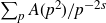 $\sum_p {A(p^2)}/{p^{-2s}}$
converge absolutely. Also,
 $F_5(s)$
is a nonvanishing analytic function for
 $\sigma \gt 1/4 + \theta$
. Since
 $\theta \lt 3/4$
,
 $F_5(s)$
converges in a neighbourhood of
 $\sigma \ge 1$
.
The product
 $F_1(s) F_2(s) F_3(s)$
meets the conditions of Lemma 2·9, so that completes the proof because
 $F_4(s) F_5(s)$
is regular and nonvanishing in a neighbourhood of
 $\sigma \ge 1$
and
 $L(s) = F_1(s) F_2(s) F_3(s) F_4(s) F_5(s)$
.
Proof of Lemma
2·9. We first show that the logarithm of L(s) converges absolutely for
 $\sigma \gt 1$
, which proves that L(s) is analytic and nonvanishing in that region. Since
 $\log(1 + Y) = Y + \mathcal O(Y^2)$
, the logarithm of one of the factors of L(s) looks like
 \begin{equation}\sum_p \left(\frac{A(p^j)}{p^{j s}} + \mathcal O\big(A(p^j)^2 p^{-2 j \sigma}\big)\right).\end{equation}
The absolute convergence of
 $F_j(s)$
in (2·43) implies (by ignoring the
 $\log(p)$
factor) that the big-
 $\mathcal O$
term above converges absolutely for
 $\sigma \gt 1- {1}/{2j}$
, so it defines an analytic function in a neighbourhood of
 $\sigma \ge 1$
.
For the main term in (2·48), if
 $\sigma \gt 1$
then by Cauchy’s inequality we have
 \begin{equation}\left(\sum_p \frac{|A(p^j)|}{p^{j \sigma}}\right)^2\le \left(\sum_p \frac{|A(p^j)|^2}{p^{(2j-1)\sigma}}\right)\left(\sum_p \frac{1}{p^{\sigma}}\right).\end{equation}
The first sum on the right above converges absolutely by (2·44) and the condition
 $2j-2+\sigma \leq (2j-1)\sigma$
for
 $\sigma \geq 1$
, and trivially so does the second sum.
Thus, L(s) is the product of three nonvanishing analytic functions in
 $\sigma \gt 1$
.
Now we consider the zeros of L(s) on
 $\sigma=1$
. Taking the logarithmic derivative of L(s) and using the same argument as above for the lower order terms, we have
 \begin{align}\frac{L'}{L}(s) & = h(s) - \sum_p \frac{A(p)\log(p)}{p^s} + 2\, \frac{A(p^2)\log(p)}{p^{2s}} +3 \,\frac{A(p^3)\log(p)}{p^{3s}} ,\end{align}
where h(s) is regular in a neighbourhood of
 $\sigma \ge 1$
.
Suppose
 $s_1,\ldots,s_J$
are zeros or poles of L(s), with
 $s_j = 1+i t_j$
having multiplicity
 $m_j$
. We have
 \begin{equation}\frac{L'}{L}(\sigma+i t_j) \sim \frac{m_j}{\sigma-1},\quad \mathrm{as}\ \sigma \to 1^+,\end{equation}
therefore
 \begin{equation}- \sum_p\left(\frac{A(p)\log(p)}{p^{\sigma + it_j}}+ 2\, \frac{A(p^2)\log(p)}{p^{2(\sigma + it_j)}}+ 3\, \frac{A(p^3)\log(p)}{p^{3(\sigma + it_j)}}\right)\sim \frac{m_j}{\sigma-1}, \quad \mathrm{as}\ \sigma \to 1^+.\end{equation}
Now write
 \begin{equation}k(s) = - \sum_{j=1}^J m_j \sum_p\left(\frac{A(p)\log(p)}{p^{s+i t_j}}+2\, \frac{A(p^2)\log(p)}{p^{2(s+i t_j)}}+3\, \frac{A(p^3)\log(p)}{p^{3(s+i t_j)}}\right)\!.\end{equation}
By (2·52) we have
 \begin{equation}k(\sigma) \sim \frac{\sum_{j=1}^J m_j^2}{\sigma-1}, \quad \mathrm{as}\ \sigma \to 1^+.\end{equation}
We will manipulate (2·53) so that so that we can use (2.44) to give a bound on
 $\sum m_j^2$
in terms of
 $M_1$
,
 $M_2$
, and
 $M_3$
.
By Cauchy’s inequality and the assumptions on
 $M_\ell$
we have
 \begin{align} |k(\sigma)| \le &\sum_{\ell=1}^3\ell \left|\sum_p \frac{p^{(1-\ell)\sigma}A(p^\ell)\log(p)}{p^{\sigma}}\sum_{j=1}^J \frac{m_j}{p^{\ell it_j}}\right| \nonumber\\ \le &\sum_{\ell=1}^3\ell \left(\sum_p \frac{p^{2(1-\ell)\sigma}|A(p^\ell)|^2 \log(p)}{p^{\sigma}}\right)^{\frac12} \left( \sum_p \frac{\log p}{p^\sigma} \biggl|\sum_{j=1}^J m_j p^{-\ell it_j} \biggr|^2\right)^{\frac12}\nonumber\\ \le & (1+o(1))\sum_{\ell=1}^3\ell\left(\frac{M_\ell^2}{\sigma-1} \right)^{\frac12}\biggl(\sum_{j=1}^J \sum_{k=1}^J m_j m_k\sum_p \frac{\log p}{p^{\sigma + i\ell (t_j - t_k)} }\biggr)^{\frac12} \nonumber\\ \sim & \frac{M_1 + 2 M_2 + 3 M_3}{(\sigma-1)^\frac12 }\left(\sum_{j=1}^J \frac{m_j^2}{\sigma-1} \right)^{\frac12} \quad \mathrm{as}\ \sigma \to 1^+.\end{align}
In the last step we used the fact that the Riemann zeta function has a simple pole at 1 and no other zeros or poles on the 1-line.
Combining (2·54) and (2·55) we have
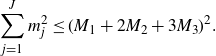 $\displaystyle\sum_{j=1}^J m_j^2 \le (M_1 +2 M_2 + 3 M_3)^2.$
Since
 $m_j\ge 1$
, we get
 $J \le (M_1 +2 M_2 + 3 M_3)^2$
, and the proof is complete.
2·9. Proof of Theorem 2·3
The proof begins the same as that of Proposition 2·1, by considering the ratio of completed L-functions:
 \begin{equation}\lambda(s) \,:\!=\, \frac{\Lambda_1(s)}{\Lambda_2(s)},\end{equation}
which is a meromorphic function of order 1 and satisfies the functional equation
 $\lambda(s)=\varepsilon \overline{\lambda}(1-s)$
, where
 $\varepsilon = \varepsilon_1/\varepsilon_2$
. First we will show that
 $\lambda(s)$
has finitely many zeros or poles in
 $\sigma \ge 1/2$
, which by the functional equation implies that
 $\lambda(s)$
has finitely many zeros or poles in the complex plane.
By the assumptions on the
 $\Gamma$
-factors, all zeros or poles of
 $\lambda(s)$
in
 $\sigma \ge 1/2$
must come from
 $L_1(s)/L_2(s)$
. Consider a local factor of that ratio:
 \begin{align}&\frac{1+a_p x + a_{p^2} x^2 + a_{p^3} x^3 + \mathcal O(p^{4\theta} x^4)} {1+b_p x + b_{p^2} x^2 + b_{p^3} x^3 + \mathcal O(p^{4\theta} x^4)}\nonumber\\ &\phantom{xxxxx}=1+(a_p - b_p) x + (a_{p^2} - b_{p^2} + b_p(a_p - b_p))x^2\nonumber\\ &\phantom{xxxxxXX}+(a_{p^3} - b_{p^3} + (b_p^2 - b_{p^2}) (a_p - b_p) -b_p (a_{p^2} - b_{p^2}))x^3 + \mathcal O(p^{4\theta} x^4)\nonumber\\ &\phantom{xxxxx}= (1 + (a_p - b_p) x) (1 + (a_{p^2} - b_{p^2}) x^2) (1 + (a_{p^3} - b_{p^3}) x^3)\nonumber\\ &\phantom{xxxxxXX}\times (1 - b_p (a_p - b_p) x^2) (1 - b_p (a_{p^2} - b_{p^2})) x^3) \nonumber\\ &\phantom{xxxxxXX}\times (1 - (2 b_p^2 - a_p b_p + a_{p^2} - 2 b_{p^2})(a_p - b_p) x^3) \nonumber\\ &\phantom{xxxxxXX}\times (1 + b_p (a_{p^2} - b_{p^2}) x^3) (1 + \mathcal O(p^{4\theta}x^4)))\nonumber\\ &\phantom{xxxxx}= (1 + (a_p - b_p) x) (1 + (a_{p^2} - b_{p^2}) x^2) (1 + (a_{p^3} - b_{p^3}) x^3)\nonumber\\ &\phantom{xxxxxXX}\times (1 + \mathcal O(p^\theta(a_p - b_p) x^2)) (1 + \mathcal O(p^{2\theta} (a_{p} - b_{p}) x^3)) \nonumber\\ &\phantom{xxxxxXX}\times (1 + \mathcal O(p^\theta (a_{p^2} - b_{p^2}) x^3)) (1 + \mathcal O(p^{4\theta}x^4)))\nonumber\\ &\phantom{xxxxx}= f_1(x) \times \cdots \times f_7(x),\end{align}
say. Let
 $F_j(s) = \prod_p f_j(p^{-s})$
.
We will show that Lemma 2·9 applies to
 $F(s+ 1/2) \,:\!=\, F_1(s+ 1/2)F_2(s+ 1/2)F_3(s+ 1/2)$
. There are three cases to consider, but it suffices to consider the weakest one:
 $\theta \lt 1/4$
and
 $B_p$
and
 $C_p$
satisfy (2·20). The assumptions on
 $A_p$
,
 $B_p$
, and
 $C_p$
involve the convergence of sums with these summands:
 \begin{equation}\frac{p\, |a_{p}-b_{p}|^2 \log(p)}{p^\sigma}, \quad \frac{|a_{p^2}-b_{p^2}|^2 \log(p)}{p^\sigma} \quad \text{and} \quad \frac{p^{-1} |a_{p^3}-b_{p^3}|^2 \log(p)}{p^\sigma}.\end{equation}
By replacing
 $a_n$
and
 $b_n$
by
 $a_n/\sqrt{n}$
and
 $b_n/\sqrt{n}$
, respectively, (equivalently, replacing s by
 $s + 1/2$
), we see that condition (2·44) applies, so
 $F(s+ 1/2)$
has finitely many zeros or poles in
 $\sigma \ge 1$
, so F(s) has finitely many zeros or poles in
 $\sigma \ge 1/2$
.
Now we check that
 $F_j(s)$
, for
 $j=4,5,6,7$
, defines a nonvanishing analytic function in a neighbourhood of
 $\sigma \ge 1/2$
. For
 $F_7$
, this requires
 $\theta \lt 1/4$
. For
 $F_4$
, comparing to
 $F_1$
we only require
 $\theta \lt 1/2$
. The same condition is sufficient for comparing
 $F_5$
to
 $F_1$
, and for comparing
 $F_6$
to
 $F_2$
.
Thus, we have established that
 $\lambda(s)$
has finitely many zeros or poles in a neighbourhood of
 $\sigma \ge 1/2$
, and so by the functional equation, finitely many zeros or poles in the complex plane.
Since
 $\lambda(s)$
has order 1, by the Hadamard factorisation theorem there exists
 $A\in \mathbb{C}$
such that
 \begin{equation}\lambda(s) = e^{A s} r(s),\end{equation}
where r(s) is a rational function.
By (2·59), as
 $|s|\to\infty$
,
 \begin{equation}\lambda(s) = C_0 s^{m_0} e^{A s} \bigl(1 + \mathcal O(s^{-1})\bigr),\end{equation}
for some
 $C_0\not=0$
and
 $m_0\in \mathbb{Z}$
. On the other hand, if
 $b(n_0)$
is the first non-zero Dirichlet coefficient (with
 $n_0\gt1$
) of
 $L_1(s)/L_2(s)$
, then by (2·56) and Stirling’s formula, as
 $\sigma\to\infty$
,
 \begin{equation}\lambda(s) = \bigl(B_0 s^{B_1} e^{B_2 s\log s + B_3 s }(1 +\mathcal O(s^{-1}))\bigr)\bigl(1 + b(n_0) n_0^{-s}+ \mathcal O((n_0+1)^{-\sigma}).\end{equation}
Comparing those two asymptotic formulas, the leading terms must be equal, so
 $B_0=C_0$
,
 $B_1=m_0$
,
 $B_2=0$
and
 $B_3=A$
.
Now let
 $s\to\infty$
along the curve
 $s= (1/2) \log(t)/ \log(n_0)+it$
. On that curve, the final factor in (2·61) equals
 \begin{align}1 + b(n_0) \frac{e^{-i t \log(n_0)}}{\sqrt{t}} &+\mathcal O\left(\frac{1}{t^{\frac12 \frac{\log(n_0+1)}{\log(n_0)}}}\right) \nonumber\\ = 1 +& b(n_0) \frac{e^{-i\frac{\pi}{4}-i t \log(n_0)}}{\sqrt{s}}+ \mathcal O\left(\frac{\log(|s|)}{s^{\frac32}}\right)+ \mathcal O\left(\frac{1}{s^{\frac12 \frac{\log(n_0+1)}{\log(n_0)}}}\right).\end{align}
We have assumed the positive integer
 $n_0$
exists, with
 $b(n_0) \not= 0$
. So there is a genuine main term of size
 $1/\sqrt{ s}$
in (2·62), which contradicts the big-
 $\mathcal O$
terms in (2·60) and (2·61). Thus
 $b(n_0)$
, the first non-zero Dirichlet coefficient of
 $L_1(s)/L_2(s)$
, does not exist, so we conclude
 $L_1 = L_2$
.
An alternate way to complete the proof uses the fact that a Dirichlet series is an almost periodic function, as in [ Reference Kaczorowski and Perelli23 ].
2·10. Proof of Theorem 2·5
We prove Theorem 2·5. The proof of Theorem 2·4 is identical, because the pth coefficients of the lifts of tensor degree m are a basis for the symmetric polynomials of degree m.
Suppose
 $L_1(s) = \sum a_n n^{-s}$
and
 $L_2(s) = \sum b_n n^{-s}$
satisfy the given conditions. As in the previous proofs, the starting point is the ratio of completed L-functions
 \begin{equation}\lambda(s) = \frac{\Lambda_1(s)}{\Lambda_2(s)} .\end{equation}
And as previously, the main step is to show that
 $L_1(s)/L_2(s)$
contributes finitely many zeros or poles in
 $\sigma\ge 1/2$
.
The theorem contains many cases, so we chose one for illustration. Suppose
 $L_1$
satisfies (vi) and
 $L_2$
satisfies (vii). By Lemma 2·8 we have
 \begin{align}\frac{L^S_1(s)}{L^S_2(s)} & =\frac{\prod_{p\ \text{good}}(1+a_p p^{-s} + a_p^2 p^{-2s}) }{\prod_{p\ \text{good}} (1+b_p p^{-s} + b_p^2 p^{-2s})} \nonumber\\ &\phantom{xxx}\times\frac{ L_1^S(2s,\mathrm{ext}^2)^{-1} \cdot h_3(3s) }{ L_2^S(2s,\mathrm{ext}^2)^{-1} \cdot L^S_2(3s,\mathrm{sym}^3) \cdot L^S_2(3s, \mathbf{1}\times \mathrm{ext}^2)\cdot h_4(4s)},\end{align}
where “p good” refers to primes which are good for both
 $L_1$
and
 $L_2$
. By the assumptions, the factor on the second line above is regular and nonvanishing on
 $\sigma \ge 1/2$
.
Writing the first factor in (2·64) as
 \begin{equation}\prod_{p\ \text{good}} \sum_{j=0}^\infty \mathcal{A}(p^j) p^{-js}\end{equation}
we have
 $\mathcal{A}(1) = 1$
,
 \begin{align}\mathcal{A}(p) & = a_p - b_p, \nonumber\\ \mathcal{A}(p^2) & = a_p (a_p - b_p) = a_p \mathcal{A}(p), \nonumber\\ \mathcal{A}(p^3) & = -(a_pb_p + b_p^2) (a_p - b_p) = -(a_pb_p + b_p^2) \mathcal{A}(p), \end{align}
and for all j,
 $\mathcal{A}(p^j) = \mathcal O(p^{j \theta^*})$
, where
 $\theta^* = \max(\theta_1, \theta_2) \lt 1/4$
. By assumption,
 \begin{equation}\liminf_{\sigma \to 1^+} (\sigma - 1) \sum_p \frac{p\, |\mathcal{A}(p)|^2 \log p}{p^\sigma}\le \mathcal{M}_1\end{equation}
for some
 $\mathcal{M}_1 \lt \infty$
. By (2·67), the bounds on
 $a_j(p)$
, and (2·68), we have
 \begin{align}\liminf_{\sigma \to 1^+} (\sigma - 1) \sum_p \frac{p^{1-2\theta^*}\, |\mathcal{A}(p^2)|^2 \log p}{p^\sigma}\le \mathcal{M}_1 , \nonumber\\ \liminf_{\sigma \to 1^+} (\sigma - 1) \sum_p \frac{p^{1-4\theta*}\, |\mathcal{A}(p^3)|^2 \log p}{p^\sigma}\le \mathcal{M}_1 .\end{align}
If we let
 $A(n) = \sqrt{n} \mathcal{A}(n)$
, then (2·67) is exactly the same as the bound on the
 $j=1$
case of (2·44) with
 $M_1 = \mathcal{M}_1$
. Also, (2·68) implies the
 $j=2$
and
 $j=3$
cases of (2·45) with
 $M_2=M_3=0$
. Finally, A(n) satisfies a partial Ramanujan bound with
 $\theta = 1/2 + \theta^* \lt 3/4$
. Thus, we can apply Corollary 2·11 to conclude that
 $\sum A(n) n^{-s}$
has finitely many zeros or poles in
 $\sigma \ge 1$
, which is equivalent to
 $L_1^S(s)/L_2^S(s) = \sum \mathcal{A}(n) n^{-s}$
having finitely many zeros or poles in
 $\sigma \ge 1/2$
.
That completes the main step in this proof. The remainder of the proof is exactly as in the proof of Theorem 2·3.
3. L-functions with an arithmetic source
The L-functions we have been discussing are defined axiomatically. All known and conjectured L-functions arise from an arithmetic or automorphic object. When such a connection is known, it is possible to prove stronger multiplicity one results.
If X is an algebraic variety then one can form its Hasse–Weil L-function L(s, X). Serre’s book [
Reference Serre45
], in Section 6·3 “About
 $N_X(p)-N_Y(p)$
,” addresses the question of what conditions on the Dirichlet coefficients imply that the two varieties have the same L-function. For example, suppose X and Y are elliptic curves over
 $\mathbb{Q}$
, with L-function coefficients a(n, X) and a(n, Y). If
 $|a(p,X) - a(p,Y)|\lt 2-\varepsilon$
for all but finitely many p, then actually
 $L(s,X) = L(s,Y)$
. Thus, for elliptic curve L-functions one can obtain the conclusion of Theorem 2·3 with significantly weaker assumptions.
If
 $\pi=\otimes\pi_p$
is a cuspidal automorphic representations of the group
 $\textrm{GL}(n,\mathbb{A}_\mathbb{Q})$
, then
 $L(s, \pi)$
is a primitive degree-n analytic L-function, satisfying all the axioms of Section 2·1, conjecturally for Axiom 4 (Temperedness). That all axiomatically defined L-functions are automorphic (with suitably restrictive axioms, of course), is likely; Selberg [
Reference Selberg44
] made that conjecture for a particular set of axioms.
Automorphic L-functions, as opposed to those that are axiomatically defined, have much stronger multiplicity one theorems because of progress on the Selberg orthonormality conjecture :
Conjecture 3·1 (Selberg Orthonormality Conjecture). Suppose that
 $L_1$
and
 $L_2$
are primitive L-functions with Dirichlet coefficients a(p) and b(p). Then
 \begin{equation} \sum_{p\le X} \frac{a(p)\overline{b(p)}}{p}=\delta({L_1, L_2}) \log\log(X)+O(1), \end{equation}
where
 $\delta({L_1, L_2}) = 1$
if
 $L_1=L_2$
, and 0 otherwise.
For the standard L-functions of cuspidal automorphic representations on
 $\textrm{GL}(n)$
, Rudnick and Sarnak [
Reference Rudnick and Sarnak40
] proved Selberg’s orthonormality conjecture for
 $\pi\cong \pi'$
under the assumption of Hypothesis H.
Rudnick and Sarnak’s Hypothesis H is the assertion
 $$ \sum_p \frac{a(p^k)^2\log^2(p)}{p^k} \lt \infty$$
for all
 $k\ge 2$
. For a given k, this follows from a partial Ramanujan bound
 $\theta\lt 1/2 - {1}/{2k}$
. Since
 $k\ge 2$
, Hypothesis H follows from the partial Ramanujan bound
 $\theta\lt 1/4$
. Rudnick and Sarnak [
Reference Rudnick and Sarnak40
] proved Hypothesis H for
 $n=2$
, 3. The case of
 $n=4$
for Hypothesis H was proven by Kim [
Reference Kim24
]. For
 $\pi\not\cong \pi'$
the Selberg Orthonormality Conjecture was proven, unconditionally for
 $n\leq 4$
and under Hypothesis H, independently by Avdispahić–Smajlović [
Reference Avdispahić and Smajlović4
] and Liu–Wang–Ye [
Reference Liu, Wang and Ye27
].
As a consequence of those results, we have:
Corollary 3·2. Suppose that
 $\pi$
,
 $\pi'$
are (unitary) cuspidal automorphic representations of
 $\textrm{GL}(n,\mathbb{A}_F)$
, and suppose
 \begin{equation} \sum_{p\le X} \frac{1}{p}\left| \mathrm{tr} A(\pi_p) - \mathrm{tr} A(\pi_p')\right|^2 \le (2-\epsilon) \log\log(X) \end{equation}
for some
 $\epsilon\gt0$
as
 $X\to\infty$
. If
 $n\le 4$
, or if Hypothesis H holds for both
 $L_\mathrm{fin}(s,\pi)$
and
 $L_\mathrm{fin}(s,\pi')$
(in particular if the partial Ramanujan conjecture
 $\theta\lt 1/4$
is true for
 $\pi$
and
 $\pi'$
), then
 $\pi=\pi'$
.
Proof. Since
 $\pi$
and
 $\pi'$
are cuspidal automorphic representations of
 $\textrm{GL}(n,\mathbb{A}_F)$
, the L-functions
 $L_1(s) = L_\mathrm{fin}(s,\pi)$
and
 $L_2(s) = L_\mathrm{fin}(s, \pi')$
are primitive L-functions. Hence, by (3·1)
 \begin{align} \sum_{p\le X} \frac{1}{p} |a(p)-b(p)|^2 & = \sum_{p\le X} \frac{1}{p} \bigl( |a(p)|^2 + |b(p)|^2 - 2 \Re(a(p)\overline{b(p)})\bigr) \nonumber\\ & = 2\log\log(X) - 2 \delta_{L_1, L_2} \log\log(X)+ O(1) \nonumber\\ & = \begin{cases} O(1) & \text{ if } L_1= L_2 \\ 2\log\log(X) + O(1) & \text{ if } L_1\not = L_2. \\ \end{cases}\end{align}
We have
 $\sum_{p\le X} ({1}/{p}) |a(p)-b(p)|^2 \le (2-\epsilon)\log\log(X)$
for some
 $\epsilon \gt 0$
. This implies that
 $\epsilon \log\log(X)$
is unbounded, and hence (3·3) implies
 $L_1(s) = L_2(s)$
. This gives us
 $\pi = \pi'$
.
Since the pth Dirichlet coefficient of
 $L(s,\pi)$
is
 $a_p = \mathrm{tr} A(\pi_p)$
, we see that condition (3·2) is similar to, but significantly weaker than, conditions like (2·20) which appear in the results for axiomatically defined L-functions. As a measure of how surprising and strong Corollary 3·2 is, we note that by the simple estimate (which follows from the prime number theorem but predates it)
 \begin{equation}\sum_{p\le X}\frac{1}{p} \sim \log\log(X),\end{equation}
and the fact that
 $1.4^2 \lt 2$
, condition (3.2) holds if
 $|\mathrm{tr} A(\pi_p) - \mathrm{tr} A(\pi_p')| \lt 1.4$
for all but finitely many p. Not only that, but the conclusion
 $\pi=\pi'$
follows from only an assumption on their traces.
For
 $\textrm{GL}(2,\mathbb{A}_\mathbb{Q})$
, the Ramanujan bound along with (3·4) implies a version of a result of Ramakrishnan [
Reference Ramakrishnan37
]: if
 $ \mathrm{tr} A(\pi_p) = \mathrm{tr} A(\pi_p')$
for
 $\frac78+\varepsilon$
of all primes p, then
 $\pi=\pi'$
. This result was extended by Rajan [
Reference Rajan38
].
Corollary 3·2 is stated for cuspidal representations, equivalently the associated L-functions are primitive, but this condition is not necessary. Suppose
 $L_1(s)=\sum A(n) n^{-s}$
and
 $L_2(s)=\sum B(n) n^{-s}$
are (not necessarily primitive) automorphic L-functions of the same degree. Write
 $A(p) = a_p + a'_p + a''_p + \cdots$
in terms of its primitive components, and similarly for B(p). Expand the sum
 $\sum ({1}/{p}) |A(p) - B(p)|^2$
and note that it must be of size at least
 $2 \log\log X$
unless the two sets of components can be paired exactly. That is, the L-functions factor into the same primitive components.
Note that the L-functions having the same degree, or having their degrees differ by 2 or more, is necessary: L(s) and
 $L(s)L(s,\chi)$
have their pth coefficients differ by 1 at almost all p.
4. Applications
By “application” we mean “deduce that two objects have identical invariants from their L-functions having similar coefficients”.
The theorems which provide a key step in applications have the form “If the L-functions of X and Y have Dirichlet coefficients
 $a_X(p)$
and
 $a_Y(p)$
which are close enough for sufficiently many p, then
 $a_X(p) = a_Y(p)$
for all good p.” The two main examples in this paper are Corollary 3·2 and Theorem 2·3. Corollary 3·2 is considerably stronger in the sense that there are fewer restrictions on the relationship between
 $a_X(p)$
and
 $a_Y(p)$
, but the cost is that it requires X and Y to arise from a cuspidal automorphic representation on GL(n).
Here we make the point that Theorem 2·3 is also useful, as long as there are L-functions which satisfy the appropriate axioms, but which are not known to be associated to a cuspidal automorphic representation. For example:
Proposition 4·1. Suppose f is a (holomorphic or Maass) newform on
 $\textrm{GL}(2)$
with trivial central character, having Hecke eigenvalues a(n). Suppose
 $g_1,\, g_2$
are cuspidal automorphic representations on
 $\textrm{GL}(N_1),\, \textrm{GL}(N_2)$
, respectively, with standard L-functions
 $L(s,g_j)=\sum b_j(n) n^{-s}$
. If
 $a(p) b_1(p)$
and
 $a(p) b_2(p)$
are close in the sense of Theorem 2·3, Then
 $N_1=N_2$
and
 $a(p) b_1(p) = a(p) b_2(p)$
for all good p, and furthermore
 $f\times g_1 = f\times g_2$
.
Proof. The pth Dirichlet coefficient of
 $L(s,f\times g_j)$
is
 $a(p) b_j(p)$
. By [
Reference Cai, Friedberg and Kaplan11
], that L-function satisfies the axioms of an analytic L-function, given in Section 2·1. Therefore we can apply Theorem 2·3.
Recent progress has shown that many L-function arise from automorphic representations on
 $\textrm{GL}(n)$
, but as long as there are analytic L-functions which have not been shown to arise in that way, there is a place for multiplicity one results which only invoke the axiomatic properties for L-functions. For example, prior to the work of Arthur [
Reference Arthur3
], the spin L-function of a Siegel modular form on
 $\textrm{Sp}(4)$
was on that list. The theorem below (which is a strengthening of Theorem 1·3) can have weaker assumptions, and a much simpler proof, thanks to Arthur’s work, but for illustration we give the version that uses Theorem 2·3.
We refer the reader to [
Reference Schmidt43
, section 2] for the following notations and definitions for Siegel modular forms on the paramodular group K(N). Let
 $k, N \in \mathbb{Z}_{\gt0}$
. Let
 $S_k^{\text{new}}(K(N))$
be the space of holomorphic Siegel modular new-forms of genus 2 with weight k, with respect to the paramodular congruence subgroup of level N. For
 $F \in S_k^{\text{new}}(K(N))$
, let
 $\mu_F(n)$
be the Hecke eigenvalue for the Hecke operator T(n) for all integers n coprime to N.
Theorem 4·2. For
 $i = 1,2$
let
 $F_i \in S_{k_i}^{\text{new}}(K(N_i))$
, with Hecke eigenvalues
 $\mu_i(n), i = 1,2$
for all n coprime to
 $N_i$
. Assume
 $k_i \geq 2$
, and the
 $F_i$
s are not Saito-Kurokawa lifts. Let
 $N = \textrm{lcm}(N_1, N_2)$
. If
 \begin{equation} \sum_{\substack{p\le X \\ p \nmid N}} p\,\log(p) \left|p^{3/2-k_1}\mu_1(p)-p^{3/2-k_2}\mu_2(p)\right|^2\ll X \end{equation}
as
 $X\to\infty$
, then
 $k_1=k_2, N_1 = N_2$
and
 $F_1$
is a scalar multiple of
 $F_2$
.
Proof. For
 $i=1,2$
let
 $a_i(n)$
be the nth Dirichlet coefficient of the degree 4 spin L-functions
 $L(s,F_i,\mathrm{spin})$
. For
 $p \nmid N$
, if
 $\alpha_{i,p},\beta_{i,p}$
are the Satake p-parameters of
 $F_i$
, then
 \begin{align*}a_i(p)&=\alpha_{i,p}+\alpha_{i,p}^{-1}+\beta_{i,p}+\beta_{i,p}^{-1}\\a_i(p^2)&= \alpha_{i,p}^2+\alpha_{i,p}^{-2}+(\alpha_{i,p}+\alpha_{i,p}^{-1})(\beta_{i,p}+\beta_{i,p}^{-1})+\beta_{i,p}^2+\beta_{i,p}^{-2}+2.\end{align*}
By [
Reference Pitale35
, section 3·4], for
 $p \nmid N$
,
 \begin{equation} \mu_i(p)= p^{k_i-3/2} a_i(p), \qquad \mu_i(p^2) = p^{2k_i-3}\left(a_i(p^2) - \frac 1p\right). \end{equation}
Hence, condition (4·1) translates into
 \begin{equation} \sum_{\substack{p\le X \\ p \nmid N}} p\,\log(p) \left|a_1(p)-a_2(p)\right|^2\ll X.\end{equation}
By [
Reference Schmidt43
, lemmas 2·3 and 2·5], both the
 $F_i$
are of general type (G). Hence, by [
Reference Schmidt43
, proposition 2·4] and (4·3), their spin L-functions
 $L(s, F_i, \mathrm{spin})$
satisfy the hypothesis of Theorem 2·3. Since the
 $F_i$
are of type (G), it is known by [
Reference Weissauer49
], that the two L-functions satisfy the Ramanujan conjecture. Hence, Theorem 2·3 implies that
 $L(s, F_1, \mathrm{spin})=L(s, F_2, \mathrm{spin})$
. This gives us
 $k_1 = k_2, N_1 = N_2 = N$
and
 $a_1(n) = a_2(n)$
for all n. In particular, (4·2) implies that
 $\mu_1(p) = \mu_2(p)$
and
 $\mu_1(p^2) = \mu_2(p^2)$
for all primes p coprime to N. Since T(p) and
 $T(p^2)$
generate the p-component of the Hecke algebra, it follows that
 $\mu_1(n)=\mu_2(n)$
for all n coprime to N. Finally, using [
Reference Schmidt43
, theorem 2·6], we can conclude that
 $F_1$
is a scalar multiple of
 $F_2$
.
Acknowledgments
We thank Farrell Brumley and Abhishek Saha for carefully reading an earlier version of this paper and for providing useful feedback on it. We are also grateful for the careful reading done by the referee who, among other things, proposed stronger results and a better way to think about applications of multiplicity one theorems, and helped us better organise the paper.



