Our brains produce a stable visual world even though the projections of the world onto our retinae jitter constantly. A multitude of mechanisms have been proposed to help explain these phenomena, and important evidence has accumulated supporting some of these mechanisms (Lee & Malpeli, Reference Lee and Malpeli1998; Ibbotson et al., Reference Ibbotson, Crowder, Cloherty, Price and Mustari2008; Melcher & Colby, Reference Melcher and Colby2008; Wurtz, Reference Wurtz2008). Much remains to be determined with regard to these issues. This study addresses a specific aspect of this larger question, namely how thalamic neurons might contribute based on timing changes.
Previous work has shown that saccades can both depress and enhance activity, depending on visual stimulation, time relative to saccades, and other factors (Leopold & Logothetis, Reference Leopold and Logothetis1998; Ramcharan et al., Reference Ramcharan, Gnadt and Sherman2001; Martinez-Conde et al., Reference Martinez-Conde, Macknik and Hubel2002; Reppas et al., Reference Reppas, Usrey and Reid2002; Sylvester et al., Reference Sylvester, Haynes and Rees2005; Kagan et al., Reference Kagan, Gur and Snodderly2008; MacEvoy et al., Reference MacEvoy, Hanks and Paradiso2008). Reppas et al. (Reference Reppas, Usrey and Reid2002) and Sylvester et al. (Reference Sylvester, Haynes and Rees2005) used full-field stimulation to minimize changes in spatial contrast during saccades. Differences between magnocellular and parvocellular neurons have been noted (Ramcharan et al., Reference Ramcharan, Gnadt and Sherman2001) but appear to depend on details of the stimulation and measures (Reppas et al., Reference Reppas, Usrey and Reid2002).
One reason we may not notice some of the jitter is saccadic suppression, involving depression of response amplitudes around saccades. However, it might also be effective to shift timing of responses. One of the goals of visual processing mechanisms might be to bridge vision across saccades (Melcher & Morrone, Reference Melcher and Morrone2003), which implies that stimuli presented before and after saccades might evoke responses that differ in timing. For one example, sustained responses might be generated before saccades and transient responses after saccades, so that responses of cells having receptive fields at different retinal positions would fire simultaneously after saccades, signaling that the same stimulus activated these positions. Price et al. (Reference Price, Ibbotson, Ono and Mustari2005) showed that latencies are reduced around saccades in middle temporal (MT) cortex, facilitating motion perception (Ibbotson et al., Reference Ibbotson, Price, Crowder, Ono and Mustari2007). This change in latency corresponds to a shift in the relation between response phase and temporal frequency, with the decreased latency suggesting that responses become more sustained. Studies in visual cortical area V1 likewise suggest that saccades lead to more sustained responses (Kagan et al., Reference Kagan, Gur and Snodderly2008; MacEvoy et al., Reference MacEvoy, Hanks and Paradiso2008). Theoretical considerations based on coding efficiency also imply that response timing in geniculate cells should vary around saccades, becoming more sustained (Dong, Reference Dong2002).
I measured response timing and amplitude of lateral geniculate nucleus (LGN) cells in an alert fixating monkey, as a function of time before and after fixational saccades. Two particularly important techniques were used in this study. First, a novel method (Saul, Reference Saul2008b) was employed to facilitate the extraction of first-order temporal kernels from responses to a variety of dense noise stimuli. This method permits calculations of reverse correlations in a continuous manner even for nonstationary systems, in this case for LGN neurons that might change their behavior around saccades. Second, the stimulus was moved on the display monitor to compensate for eye movements, so that responses to spatially localized stimuli could be analyzed (Gur & Snodderly, Reference Gur and Snodderly1987; Tang et al., Reference Tang, Saul, Gur, Goei, Wong, Ersoy and Snodderly2007). Spatial contrast changes due to saccades were minimized.
Both parvocellular and magnocellular neurons showed a prominent decrease in response amplitudes around saccades. Timing shifted as well, with cells becoming more sustained around saccades. I argue that such timing changes could be key in understanding vision around saccades.
Materials and methods
A rhesus macaque (Macaca mullata) was implanted with a head-holding device and trained to perform a fixation task. Procedures were described in detail in Tang et al. (Reference Tang, Saul, Gur, Goei, Wong, Ersoy and Snodderly2007) and Saul (Reference Saul2008a). Eye coils were implanted in a separate surgery. All interventions complied with the NIH guidelines for the care and use of animals and with the approval of the Institutional Animal Care and Use Committee of the Medical College of Georgia.
Single neurons in LGN were recorded extracellularly. Guide tubes were implanted under sedation with ketamine/xylazine (10/1 mg/kg). Some cells were recorded with implants that included three guide tubes spaced about 800 μm apart. Other cells were recorded using a single guide tube. Electrodes were pulled from 40-μm diameter platinum–tungsten fibers insulated with quartz glass. Tips were ground to about 5 μm of exposed metal, at the end of a taper about 15 μm long. Repeated penetrations were made over many days, with consistent depth readings (Saul, Reference Saul2008a). Eccentricities ranged from 2 to 19 deg, with a mean of 8 deg.
The monkey performed a fixation task during 5-s trials. A cue tone warned that a trial would begin, and a red light-emitting diode (LED) turned on. The monkey needed to press and hold a lever within 500 ms of the onset of the LED and acquire the LED and maintain fixation on it until it was extinguished after 5000 ms. She then had to release the lever. Successful completion of this sequence was rewarded with 0.2–0.5 ml of water. Trials were repeated at an interval of about 10 s. Every hour or so, food was offered to provide a break and to stimulate thirst.
A fixation window with a radius of 1 deg was present electronically during most experiments, but this monkey rarely looked outside it, so very few trials were terminated due to loss of fixation. However, small saccades within the window, as well as drifts, were common.
Action potentials were isolated with a single threshold that triggered storage of the analog voltage at 25 kHz over a 3.2-ms period starting 0.2 ms before the trigger. Spikes from a single cell were separated off-line from any other spikes and from artifacts by applying a variety of methods interactively. The main method was setting a criterion for a similarity measure between the potential spike waveform and the mean waveform across all the spikes. Cleaned spike trains were then converted to histograms for each trial with 6.25-ms bins.
Cells were first tested manually and then under computer control. Generally, a small spot was placed in the receptive field center, and its luminance and color were modulated in time (mean luminance was 15 cd/m2). For the LGN data presented here, the stimuli were fields of small contiguous bars, each of which was modulated independently of the other bars. These spatiotemporal noise stimuli took several forms.
For 15 LGN cells, luminance was modulated, using either binary or ternary white noise, or for 3 of the cells, natural noise. The natural noise was based on the following second-order autoregressive sequence:

where xi is the i-th luminance value in the sequence, and v is a uniformly distributed random value between −1 and 1. Contrast was enhanced by applying a sigmoidal function to these values. This type of noise tends to maintain the luminance around the same level, as well as continuing in the same direction as previous changes. The power spectrum is relatively flat as a function of logarithmic frequency.
Chromatic modulations were used for six of the cells. On every other frame, the color was set to one of six colors that were from pairs of cone-isolating colors or in three cases to one of the colors in the entire monitor gamut. For the first case, the cone-isolating colors were determined by measuring the monitor spectra with a SpectraScan spectrometer (Photo Research, Chatsworth, CA), then calculating the dot products by cone fundamentals.
In all cases, no spatial correlations were imposed. Each position was stimulated independently and analyzed separately. The response of the cell to each 5-s trial was correlated with the stimulus at each position. These correlations were computed with the wavelet technique (Saul, Reference Saul2008b). Briefly, both stimulus and response were transformed to a time–temporal frequency representation. The response was then divided by the stimulus at each time and frequency, giving a set of samples of the frequency domain version of the first-order kernel assumed to underlie much of the response mechanism. The samples at each frequency were median filtered in amplitude to remove artifacts, then averaged in the complex plane to yield the kernel estimate. These estimates were averaged over all the trials. From these calculations, maps were obtained of the receptive field in space and time. The position that produced the impulse response function with the largest peak was thus found, and the computations were repeated, but the samples for that strongest position were not averaged. Instead, they were added to arrays that accumulated the frequency domain kernel as a function of time relative to saccades. Units for impulse responses are spikes per second per full range of contrast, or they could be taken as conditional probabilities, and are omitted because of their nonintuitive nature.
Eye position was measured via search coils sutured to the sclera of each eye. Signals from the eye coils were amplified 40× before leading them to the demultiplexer (Remmel Labs, Katy Texas). Horizontal and vertical eye positions were sampled at 200 Hz from the dominant eye. Changes in eye position as small as a few minarc could be measured reliably (Tang et al., Reference Tang, Saul, Gur, Goei, Wong, Ersoy and Snodderly2007).
Stimuli were shifted on the monitor to largely compensate for the eye movements. The horizontal and vertical eye position outputs were led to inputs on the video card (VSG 2/3; Cambridge Research Systems, Kent, UK) and thereby were instantaneously added to the stimulus position (Gur & Snodderly, Reference Gur and Snodderly1987, Reference Gur and Snodderly1997; Snodderly & Gur, Reference Snodderly and Gur1995; Tang et al., Reference Tang, Saul, Gur, Goei, Wong, Ersoy and Snodderly2007). Therefore, maps show retinotopic coordinates rather than external visual space. However, these stimulus shifts cannot be made until the next video frame, so there is a delay of up to 6.25 ms, which means that saccades cause retinal slip during this time. Because this could conceivably affect the results of this study, an additional correction was made in the off-line analyses. When the eyes moved farther than one stimulus bar width during one frame, the stimulus record was corrected to estimate the actual stimulus presented to that retinal position during the following frame. This estimate is imperfect because the actual stimulus depends on the relative timing of the eye position signal that was sampled at 200 Hz and the frame refresh at 160 Hz, as well as potential delays in software execution and position on the monitor that produces a delay due to raster scanning. Those delays are probably negligible, but the unknown relative phases of the eye position and drawing signals mean that the total delay is somewhere between zero and two frames, 0–12.5 ms, but probably distributed with a strong mode around 6 ms.
Saccades were defined as changes in eye position with speeds greater than 10 deg/s. This criterion differentiated well between slow movements (such as drifts) and saccades. Note that the saccades here were small, generally on the order of 20–40 minarc. The speed criterion used meant that very small saccades, less than about 10 minarc, were rejected. The time of saccade occurrence was taken as the first bin for which the speed exceeded the criterion.
Most cells were tested with 8–20 different pseudorandom sequences, repeated 3–12 times, for total testing times ranging from 5 to 20 min. Note that the actual time a single run took is much more than the testing time since an intertrial interval of at least 5 s was always present, and the monkey took breaks occasionally.
Geniculate neurons were classified as parvocellular (P), magnocellular (M), or koniocellular (K). Anatomical locations were reconstructed based on depth readings over many days of recordings, along with eye dominance (Saul, Reference Saul2008a). The laminar patterns were clear for almost all cells. In addition, chromatic opponency was tested for many cells. A cell was called P if it was recorded in one of the four dorsal layers 3–6 and if it had L–M cone opponent responses. M cells were recorded in layers 1 and 2 and had nonopponent responses. Cells with strong S-cone input are not included here.
Results
Fixational eye movements
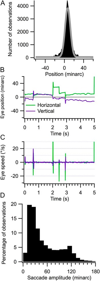
The monkey was highly trained in fixation and therefore maintained eye position near the target. On some trials, no saccades were made. However, as with all monkeys and humans, fixational eye movements were generally present. Fig. 1A shows a histogram of eye position averaged over a typical run (see the M46 LGN results in Fig. 3 of Tang et al., Reference Tang, Saul, Gur, Goei, Wong, Ersoy and Snodderly2007, for more extensive data). She maintained her eyes on the fixation target with a s.d. of 8 minarc (half-width of Gaussian fit, note that the histogram is kurtotic, more peaked than a Gaussian—the nonzero offset of the mode is due to the slightly arbitrary setting of the offsets on the eyetracker by the user). An example of a representative trial is shown in B, with the horizontal and vertical eye positions shown as green and purple traces, respectively. Four saccades were made during the trial, neglecting when she looked away at the end, and these were captured by differentiating the eye position records and setting a criterion of speeds that exceeded 10 deg/s (C). Away from these saccades, eye speeds were much slower. Very few small microsaccades with speeds slower than 10 deg/s occurred during active fixation in this monkey. On average, over all runs analyzed here, saccades occurred 2.2 times per second.
Fixational eye movements. Horizontal eye position sampled at 200 Hz over 63 trials was collected into the histogram in (A) (filled black bins). A Gaussian fit to this histogram is shown by the gray trace. Horizontal and vertical eye position records are illustrated for a single trial in (B). These were differentiated and plotted in (C). A speed criterion of 10 deg/s was applied to accept saccades. The distribution of amplitudes of all the 18,774 saccades used in this study is shown in (D).

The saccades accepted had amplitudes ranging from about 10 minarc to 3 deg. The histogram in Fig. 1D compiles all the saccades used in this study, totaling 18,774 across 21 runs. Saccades typically had amplitudes around 20 minarc. About 70% of the saccades had amplitudes less than 1 deg. Because of this limited variance, effects of saccade size on the results were not considered. Previous work showed that amplitude changes in LGN neurons do not depend strongly on saccade size (Reppas et al., Reference Reppas, Usrey and Reid2002). Large saccades were mostly suppressed because the monkey had been highly trained that trials would be terminated without reward if fixation was broken. Blinks were infrequent during the 5-s trials.
Data extraction
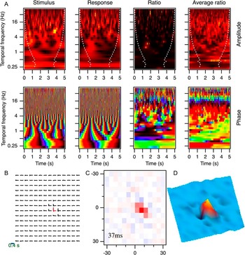
The main results here come from 21 cells in the left LGN of an alert monkey, including 17 P cells and 4 M cells. Cells were tested with dense noise stimuli and analyzed using wavelet transforms (Saul, Reference Saul2008b; Fig. 2). For each trial, and for each tested position, the stimulus and response were transformed to their wavelet representations (left side of Fig. 2A). That is, they were cast as complex (i.e., comprising both amplitude and timing) functions of time and temporal frequency. The response was then divided by the stimulus, providing an estimate of the first-order kernel relating them, at a series of times during the trial (ratio panels in Fig. 2A). These were averaged across all 76 trials in this run (rightmost panels in A). The amplitude plots in A (upper row) are functions of time (horizontal axis) and temporal frequency (vertical axis). Warmer/brighter colors correspond to stronger amplitudes. The dashed lines delineate the “cone of influence” outside of which the values are less reliable and were therefore not used (Saul, Reference Saul2008b). The phase plots (lower row) use colors ranging from dark to bright and back to dark, or from black through purple, blue, green, yellow, red, and back to black over a cycle.
Wavelet analysis. A parvocellular neuron was tested with luminance-modulated ternary white noise. Stimuli and responses were transformed to time–temporal frequency space. In (A), amplitude and phase are shown in this space for a single trial (left panels) for the stimulus, the response, and their ratio. The rightmost panels show the average ratio across all 76 trials. The data in (A) refer to the position with the strongest response. Warmer colors correspond to stronger amplitudes, and colors cycle around the spectrum with the phase values, yellow indicating 0 cycles and black 0.5 cycles. The white dashed lines in the amplitude plots designate the cone of influence, indicating that early and late times were discarded for low frequencies because of insufficient sampling times. The entire space–time map is shown in (B), plotting the first 400 ms of the impulse responses at 196 positions. The colored impulse response had the largest peak response, and this position is used in panel (A). The spatial slice at 37 ms is plotted in (C). The 14 × 14 grid spanned 60 minarc in each dimension. The color range is blue to white to red, representing negative to positive values of the impulse responses at 37 ms, which is the time of the peak of the strongest impulse response. The map is shown again as a three-dimension plot in (D) with a different color scale and orientation that make the weak surround more apparent.

The ratio data represent samples of the cell’s first-order kernel. The single trial example in the third column has little apparent structure in its amplitude, but the phase results provide a glimpse of the averaged phase, with a relatively consistent sequence across frequencies for many time points. The average over trials on the right shows the sequence more clearly at high frequencies. The averaged amplitudes were not strongly tuned in this case, although a falloff can be seen at high frequencies.
The data in Fig. 2A were from the position with the strongest response. The results from all positions (this cell was tested over a 14 × 14 grid spanning 1 deg along each axis) are shown in B. These are impulse response functions obtained by inverse transforming frequency domain kernels. These frequency domain kernels were taken from the average ratio data, as in the example on the right in A, after performing averaging across time (see Saul, Reference Saul2008b, for details). The spatial position that yielded the strongest response is indicated in color. Positions outside the small receptive field yielded vanishing impulse responses compared to the central positions. The 0.4-s scale bar is the time base for these impulse response functions.
A purely spatial map was derived from these spatiotemporal kernels by looking at the values at the peak time for the strongest position. This time, as seen more clearly in Fig. 3, was 37 ms in this example. Fig. 2C shows the spatial map, with red representing bright excitation and blue representing dark excitation. The impulse responses have units of spikes per second per unit contrast but have been normalized to peak values of ±1 throughout. The colors in C have been scaled across this full range, so that here the blue points are unsaturated because the lowest levels of the impulse response functions are only slightly below 0, not approaching −1 at any position. This is shown differently in the plot in D, where the colors have not been scaled uniformly. The small dark depressions provide a suggestion of the weak inhibitory surround, which peaked slightly later than the excitatory center.
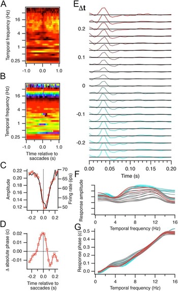
Responses relative to saccades. Data shown here were derived from the position with the strongest responses in Fig. 2. The response-to-stimulus ratios were reordered based on the time relative to each saccade and averaged for each of those times, as shown in (A) (amplitude) and (B) (phase). After binning these frequency domain kernels at 25-ms intervals, they were inverse transformed to the impulse response functions in (E). The numbers for Δt, time relative to saccades, are at the centers of these 25-ms bins. Black lines give the zero level. The amplitudes and absolute phases for these averaged data for the central 500 ms are shown in (C) and (D). Amplitudes (red trace and left axis) are the RMS values of the impulse responses after normalizing to the maximum value across time and Δt. Superimposed on the RMS amplitude in (C) is the saccade-triggered firing rate (black trace and right axis). Absolute phase values are the intercepts of the phase versus temporal frequency regressions, weighted by the amplitudes, relative to the average across Δt. The frequency domain versions of the impulse response functions in (E) are shown in (F) (amplitude) and (G) (phase). There were 1320 saccades during the 76 trials in this run and 26,034 spikes.

The preaveraging frequency domain kernels for each trial (i.e., data like those in the third column of Fig. 2A) were also reassigned to times relative to saccades. For instance, if there was a saccade at 2.0 s, then the kernel originally at 1.5 s would be associated with the relative time of −0.5 s (Fig. 3A and 3B). This operation was performed for each saccade, so kernels could be assigned to more than one bin, relative to more than one saccade. However, saccades were infrequent enough that this was seldom the case for times within a few hundred milliseconds of saccades.
Amplitude and timing around saccades
Fig. 3A manifests a decrease in amplitude around the time of saccades. Responses particularly decreased in strength between about 4 and 32 Hz. Phase values, shown in B, seemed to be less affected by saccades, although some small disruptions are present.
The frequency domain kernels for each of the times relative to saccades were inverse transformed to show the impulse response functions at a series of intervals before (negative values of Δt and green colors) and after (positive Δt values and red colors) saccades (Fig. 3E). Averaging was performed over 25-ms segments before computing the inverse transforms. The impulse responses at most times relative to saccades varied little but became weaker around the time of saccades.
The strength of these kernels was quantified by measuring the root-mean-square (RMS) amplitude of the impulse responses. Only the first 200 ms of each impulse response was considered for these analyses. All the impulse response functions were normalized to the peak or trough of the strongest impulse response. The RMS amplitude therefore has values less than 1 (Fig. 3C). The dip in amplitude around the time of saccades is clear. Amplitude drops by about 50% and recovers in less than 200 ms. This is compared with the conventional saccade-triggered average firing rate (black trace and right axis), which is similar. An advantage of the wavelet method is that it performs better at estimating kernels with limited data, converging more quickly though with slightly less accuracy than the conventional methods (Saul, Reference Saul2008b). In the present context, it enables both amplitude and timing measurements to be extracted from the nonstationary system of LGN cells whose behavior is modulated by intermittent saccades.
Timing was measured from the frequency domain versions of the kernels. Linear regression was performed on the phase versus temporal frequency data (Fig. 3G), weighted by the amplitudes (Fig. 3F). The two parameters of the lines fit to the data are called latency (slope) and absolute phase (intercept at 0 Hz) (Saul & Humphrey, Reference Saul and Humphrey1990). Absolute phase characterizes when responses occur to arbitrary stimuli: transient nonlagged cells have absolute phase values approaching quarter cycle phase leads (−0.25 c), sustained nonlagged cells have absolute phase values just less than 0 c, sustained lagged cells have absolute phase values just greater than 0 c, and transient lagged cells have absolute phase values approaching a quarter cycle phase lag (0.25 c).
In this example, timing was retarded around saccades (Fig. 3D). This sustained ON P cell had an absolute phase value of about −0.05 c (0 cycles is completely sustained ON, and −0.25 c is completely transient ON). Timing became slightly more sustained around saccades, as the secondary inhibition weakened relative to the primary excitation (gray traces in E—compare with Fig. 3 in Reppas et al., Reference Reppas, Usrey and Reid2002). Note that the excitatory mode also weakened, though relatively less. The weakened secondary inhibition in the impulse responses changes the amplitude tuning slightly (Fig. 3F) but, more importantly here, retards phase values at low frequencies (Fig. 3G).
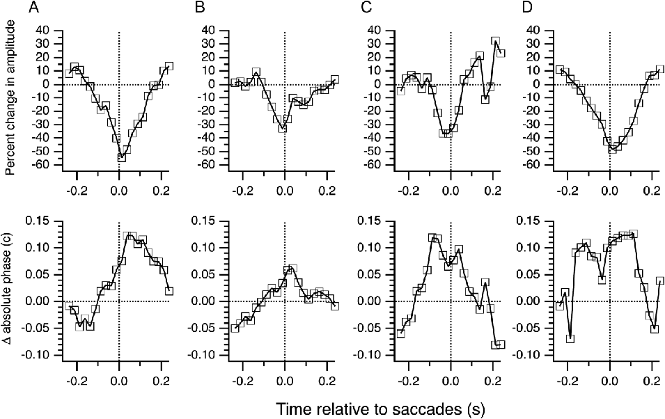
The example in Figs. 2 and 3 illustrates effects of fixational saccades on the strength and timing of the responses but is shown primarily to illustrate the methods, as well as the consistency of the results. Four more examples are presented in Fig. 4. Amplitude and absolute phase changes are plotted relative to the averages across ±1 s. Other baselines were examined with no major differences in results. The M cell in A had a clear dip in amplitude that began before saccade onset and lasted until well after the saccade. Timing shifted from transient lagged to transient nonlagged of the opposite sign (i.e., the initially stronger secondary phase of the impulse response became weaker than the primary phase), starting just before saccades and recovering within 200 ms. The M cell in B had weaker effects but became slightly more sustained just after saccades. The P cell in C had only a small change in amplitude but a large shift in timing, again from transient lagged to transient nonlagged. The M cell in D showed strong effects over a long period around saccades, again losing responsiveness and becoming more sustained. In almost all cases, amplitudes decreased around saccades and response timing was retarded.
Examples of saccade effects. Changes in amplitude and absolute phase are shown for four LGN cells. Values are relative to averages between −1 and +1 s around saccades (horizontal lines). (A) A transient lagged-OFF M cell. (B) A sustained nonlagged-OFF M cell. (C) A transient lagged-OFF P cell. (D) A transient nonlagged-OFF M cell.

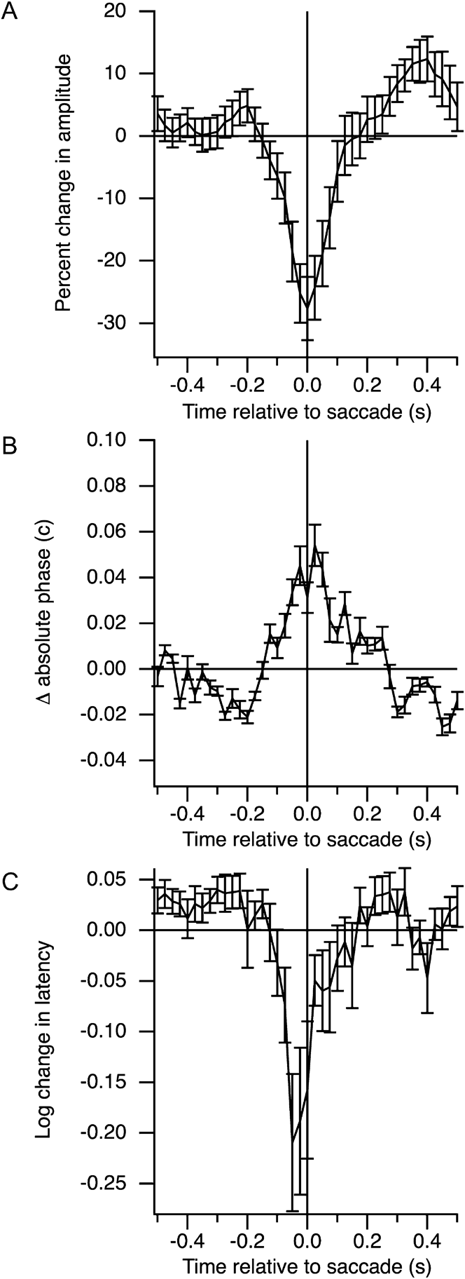
Over a population of 21 LGN cells, the averaged changes in amplitude and phase are summarized in Fig. 5. These data have been normalized to show the changes relative to the average of the values over ±1 s around saccades. Amplitudes were clearly depressed around saccades, with a small rebound after about 300 ms (A). The rebound seen here does not match that seen by Reppas et al. (Reference Reppas, Usrey and Reid2002), who observed slightly enhanced responses from about 50 to 200 ms postsaccades. Absolute phase changes were less consistent than amplitude changes but showed an increase around saccades (B). Latency, the slope of the phase versus temporal frequency relation, decreased before saccades (C) but was highly variable. The decrease in latency arises directly from the increase in absolute phase, as phase was retarded specifically at low frequencies (Fig. 3G). The results suggest that effects are somewhat symmetric around the time of saccades, starting about 100 ms prior to saccades and recovering within about 100 ms.
Population effects. Averaged across 21 LGN cells, amplitude (A), absolute phase (B), and latency (C) were affected by saccades. Baselines were set as the average across 2 s around each saccade. Mean values with s.e.s are shown.

In these experiments, the visual effects of saccades are present only for less than 12.5 ms because of the eye position compensation system. This brief retinal slip could affect responses over a longer period, however, with a latency and duration that might influence the measurements over some tens of milliseconds following saccades. The fact that effects start prior to saccades argues that additional factors alter the cell’s temporal responses.
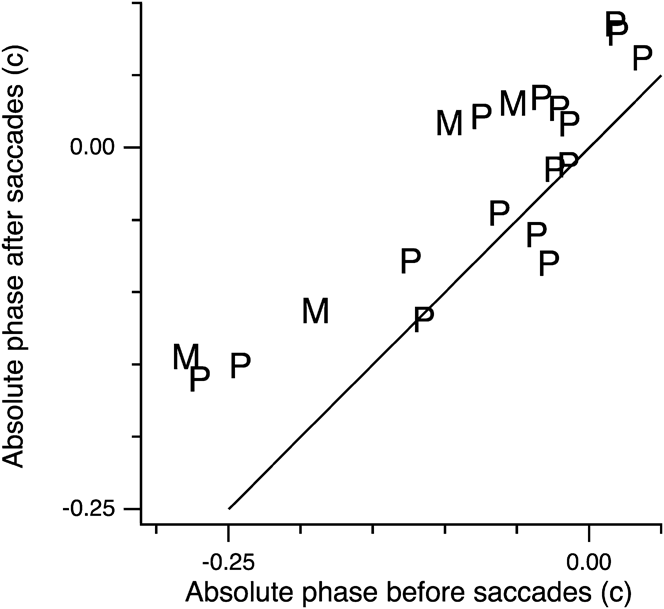
The changes in absolute phase could depend on the baseline absolute phase of each cell. For instance, transient cells might become more sustained but sustained cells might become more transient. Fig. 6 illustrates the results in more detail, showing the absolute phase of each neuron 250 ms prior to saccades along with their absolute phase values right after the saccades. Parvo- and magnocellular neurons are separated, as well. Along the solid line, no change occurs. The data fall mainly above this diagonal, so the majority of cells had increased absolute phase after saccades, as suggested by the average (Fig. 5). Sustained cells (presaccade absolute phase values near 0) tended to become more sustained and cross into lagged absolute phase values. Transient cells (presaccade absolute phase values near −0.25) became more sustained. These findings mean that responses lasted longer after saccades in almost all cases.
Timing around saccades. Absolute phase is plotted before and after saccades. Absolute phase was averaged for 100-ms periods, starting 250 ms before saccades, or starting at the times of saccades. Absolute phase has been shifted by a half-cycle for OFF-center cells. M and P cells are indicated.

Similar results were seen for other choices of time intervals for pre- and postsaccadic absolute phases. Consistent with the average data in Fig. 5, absolute phase increased for almost all cells prior to saccade onset. The effects faded gradually after 150 ms, especially for the more transient cells.
Absolute phase values were also compared by first smoothing the values across the ±1-s interval with a Gaussian window with a width of 125 ms. Values in the central 200 ms were then compared to the values outside that interval, using a t-test with a criterion of P < 0.05 to reject the null hypothesis that the means were the same. This is a conservative test because for most cells, the effects were not seen throughout the ±0.1-s interval chosen. The null hypothesis was rejected in 16 of the 21 cells. Thus, absolute phase was significantly retarded around the time of saccades in 76% of the LGN neurons.
No differences were noted between cells tested with chromatic versus luminance modulations or between white versus natural modulations, for this small sample. Geniculate neurons respond with similar timing to different stimulus types, as long as contrasts are similar.
Remapping
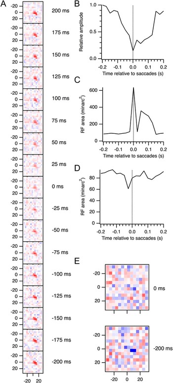
Several studies have demonstrated remapping of receptive fields around saccades (Duhamel et al., Reference Duhamel, Colby and Goldberg1992; Walker et al., Reference Walker, Fitzgibbon and Goldberg1995; Umeno & Goldberg, Reference Umeno and Goldberg1997; Nakamura & Colby, Reference Nakamura and Colby2002), meaning that the spatial receptive field shifts prior to saccades in a predictive manner. Fig. 7A shows the receptive field maps from the cell in Figs. 2 and 3 for a series of time points relative to saccades. All these maps represent the spatial receptive field at a visual latency of 37 ms, where the peak responses occurred. Because these maps were averaged over all saccades, one would not expect any shifts in a given direction. However, the receptive field might be expected to broaden around saccades. Such broadening should be easily measurable, thanks to the high resolution of the maps enabled by compensation for eye movements (Tang et al., Reference Tang, Saul, Gur, Goei, Wong, Ersoy and Snodderly2007). Receptive field diameters were often smaller than even small fixational saccades.
Absence of remapping. (A) The spatial receptive field of the cell illustrated in Figs. 2 and 3 is shown at a range of times relative to saccades. All these maps are slices of the spatiotemporal kernels at 37 ms. Numbers to the right of the maps indicate the time relative to saccades. Numbers on axes give position in minarc. (B) Amplitudes of two-dimensional Gaussian fits to the maps in (A). Units have been normalized to the maximum amplitude. (C) Areas of the Gaussian fits at half-height. (D) Areas computed from smoothed subsampled maps, at half-height. (E) Slices of the spatiotemporal kernel at 56 ms, near the trough of the secondary mode of the impulse response functions shown in Fig. 3. Maps are shown for 200 ms before saccades and at the time of saccades. All maps in (A) use the same color scale, but the two maps in (E) use an expanded color scale as they have weaker amplitudes.

To compute receptive field size, two-dimensional Gaussians were fit to these maps. Amplitudes of these fits are shown in Fig. 7B. As for the single pixel data shown in Fig. 3, amplitudes decreased around saccades. The amplitude at the time of saccades is less than a third of the peak amplitude away from saccades. The areas of the fitted Gaussians were computed at half of the peak height. Near saccades, these areas appeared to increase (Fig. 7C). However, this effect was entirely artifactual due to the decreased amplitudes. That this is an artifact is clear from several considerations. First, examination of the raw maps in Fig. 7A shows that such a large change is not obvious. Second, the magnitudes of the increased areas are far beyond what one might expect, representing several times the area away from saccades (~300–400 minarc2 compared to 100 minarc2). Third, these increases only appear at 5 time points relative to saccades and are not consistent over a range of times. Fourth, an alternative method of computing area did not confirm this finding. In Fig. 7D, areas are shown as calculated from smoothed versions of the maps. The original maps in Fig. 7A were subsampled from 14 × 14 to 100 × 100 points, slightly smoothed using a Gaussian with a width of 6 minarc, and the number of pixels with values above half-maximum for that map were counted. No increase in area was seen around saccades using this method. Additional smoothing did not lead to increased areas around saccades.
No clear evidence of spatial remapping was found in the LGN cells sampled in this study using the analyses illustrated in Fig. 7. The timing changes observed at the receptive field center might extend to other positions, however, and receptive fields might expand spatially at other times than the time where the kernel peaks for the center pixel. Unfortunately, responses become too weak to obtain reliable measurements at times later than this peak time. In particular, the timing change around saccades manifests as a profound weakening of the secondary inhibition, and spatial maps, at times where this inhibition is clear away from saccades, do not show structure near saccades. Fig. 7E shows two maps computed at 200 ms before and at the time of saccades, at a visual latency of 56 ms. This latency is where the secondary inhibition was strongest (Fig. 3F). Although the rebound responses can be seen at the receptive field center, and at a few neighboring points in space for times away from saccades, the maps near saccades are insufficient for computing areas.
Discussion
Traditionally, investigators have paid attention to the effects of saccades on response amplitudes, mostly looking for the neural bases of saccadic suppression. These effects have been observed, but the results are mixed, with some studies showing decreases in responses, other studies not finding obvious suppression, others seeing increased responsiveness, as well as both suppression and enhancement separated in time (Reppas et al., Reference Reppas, Usrey and Reid2002). Numerous factors contribute to this stew, such as brain area, cell type, saccade type, and visual stimulation (Sylvester et al., Reference Sylvester, Haynes and Rees2005; Sylvester & Rees, Reference Sylvester and Rees2006). An alternative view is explored here that what might change is response timing. In addition, fixational saccades were examined rather than voluntary saccades.
Changes were most commonly observed to consist of a decrease in amplitude and a shift in response timing. Sustained cells became more sustained, or lagged, around the time of saccades, whereas transient cells became less transient. These timing changes recapitulate what was seen by Reppas et al. (Reference Reppas, Usrey and Reid2002) who used full-field stimulation and large voluntary saccades and examined impulse response functions. The shift in timing typically occurred at the time of the saccade, or tens of milliseconds before, and persisted for about 200 ms. The increase in absolute phase (which depends primarily on the phase at low frequencies), often accompanied by a decrease in latency (the slope of phase vs. frequency), arose from the fact that saccades primarily affected responses to low temporal frequencies. This is consistent with the slow time course of extraretinal effects seen in previous studies (Kagan et al., Reference Kagan, Gur and Snodderly2008).
Expected effects of LGN timing changes
What are the likely consequences of these changes in absolute phase? Consider responses of a cortical cell that receives input from a set of geniculate neurons with a range of spatial receptive field locations. The absolute phase of the inputs progresses across the receptive field, decreasing in the preferred direction. This permits the cell to respond well to a stimulus moving in that preferred direction. If a small saccade occurs while the optimally moving stimulus is in the receptive field, what might be expected? If the saccade is in the direction opposite the motion of the stimulus, the stimulus will jump in retinal coordinates to positions farther along in its trajectory, moving too rapidly past intermediate positions to stimulate retinal and geniculate neurons with receptive fields in those locations. This jump would reduce the response of the cortical cell, as the integration of the inputs would be diminished. As observed in this study, the timing of the inputs is retarded, so that some of this lost input would be restored. The jump forward in space caused by a saccade is partly compensated by a jump backward in time.
The extent to which this retarded timing would improve responses depends on the direction of the saccade relative to the cortical cell’s preferred direction, the size of the saccade, and the relevant spatial frequencies in the stimulus. The component of the saccade opposite the cell’s preferred direction, as a fraction of the spatial period of the stimulus, might be expected to match the timing changes, which averaged about 0.05 c at their peak (Fig. 5). For a 12 minarc (0.2 deg) saccade opposite a cell’s preferred direction, the stimulus component at 0.25 cpd (0.2 deg × 0.25 cpd = 0.05 c) would be fully compensated. For cells with preferred directions away from that of the saccade, higher spatial frequencies would be compensated. Note that for saccades along a cell’s preferred direction, the stimulus would jump backward along its trajectory and would therefore stimulate the cell adequately, at least as well as expected without the timing changes. Space–time diagrams of stimuli and receptive fields might make these arguments clearer but suffer from the need to think through the convolutions, whereas consideration of phase makes the calculations simple, as above.
The decrease in amplitude around the time of saccades might be expected to eliminate these enhancements of responses due to timing changes. However, the amplitudes of the geniculate inputs to cortex may not be as important as their timing, given the integration that occurs among excitatory and inhibitory elements. Consistent with previous reports, V1 neurons, stimulated and analyzed in the same manner as the LGN cells shown in this report, exhibited a variety of effects, with many cells showing enhanced amplitudes around saccades (data not shown). Cortical amplitudes depend on geniculate amplitudes only when timing is also taken into account. Bair & O’Keefe (Reference Bair and O’Keefe1998) demonstrated that middle temporal cortex (area MT) neurons respond to moving stimuli in the presence of fixational saccades in a manner consistent with these arguments. Ibbotson et al. (Reference Ibbotson, Price, Crowder, Ono and Mustari2007) showed postsaccadic enhanced responses in MT and dorsal medial superior temporal (area MSTd) cortex during an ocular following task and provided arguments that these effects could be inherited from LGN, though their discussion concentrated on amplitude changes.
In cortical area MSTd, latencies to flashed texture patterns shortened around the time of saccades (Ibbotson et al., Reference Ibbotson, Crowder, Cloherty, Price and Mustari2008; Crowder et al., Reference Crowder, Price, Mustari and Ibbotson2009). This might be related to perceptual time compression (Morrone et al., Reference Morrone, Ross and Burr2005; Binda et al., Reference Binda, Cicchini, Burr and Morrone2009), as two stimuli flashed briefly before and just after saccades would evoke a response time difference in MSTd smaller than the stimulus time difference. The absolute phase changes in LGN reported above are consistent with shortened latencies. To see this, one must recognize that the brain does not compute latencies directly but instead derives them from how phase varies with temporal frequency. As illustrated in Figs. 3G and 5C, these latencies are shorter before saccades. Phase is retarded to a greater extent at low temporal frequencies than at higher frequencies, reducing the slope, which is the latency.
Binda et al. (Reference Binda, Cicchini, Burr and Morrone2009) described a model for the perceptual spatiotemporal distortions they observed around the time of saccades. The key aspect of their model is a spatiotemporally oriented mechanism that traces the saccade trajectory. Note that their transfer function does not correspond to a receptive field mechanism since it is oriented in the opposite direction. Their psychophysical model could be implemented by physiological mechanisms, however, with these spatiotemporal profiles generated by temporal shifts of the kind observed in the present study. For example, more sustained responses at receptive field positions stimulated before saccades compared to those stimulated after saccades would combine to produce spatiotemporally oriented alterations in cortical receptive fields. Modeling flash responses in terms of impulse response functions or response phase might help to explain the temporal reversal that occurs about 70 ms before saccades. For example, this may correspond to a steep change in latencies, as suggested by Fig. 5C above. Terao et al. (Reference Terao, Watanabe, Yagi and Nishida2008) showed that, in addition to saccades, decreases in visibility, such as those induced by flicker or low contrast, also evoke perceptual temporal compression. They argued that these effects are due to weak transient signals under the low visibility conditions. Again, it will be important to test physiological mechanisms, but it seems likely that not just changes in amplitude but also changes in timing could account for shifts in the transient/sustained behavior of the visual system.
Seeing across saccades
Response timing is the fundamental property of neurons. Even more important than how strongly a cell responds is when it responds. To understand how this interacts with the issue of stable vision in the presence of head and eye movements (Melcher & Colby, Reference Melcher and Colby2008), consider a highly simplified situation. A single static object sits in the visual field. The object’s position on the retina shifts slightly from before to after a fixational saccade. Imagine that cells signal the location of the object by their activity. If cells only fired when the object was present in their receptive fields, then the object location would seem to jump from before to after a saccade, contrary to experience. Instead, sustained and lagged responses permit activity to persist after a saccade removes the object from receptive fields. Persistent activity from cells with receptive fields at the presaccade location overlaps with that of cells with receptive fields at the later location. After the saccade, the activity would be interpreted in this oversimplified scheme as locating the object at both positions. In a more realistic scheme, the conjunctive firing of these sets of cells could provide the association needed to interpret the shift as due to a saccade. The brain can thereby signal to disregard a saccade (“remapping”; Duhamel et al., Reference Duhamel, Colby and Goldberg1992; Nakamura & Colby, Reference Nakamura and Colby2002; Melcher & Colby, Reference Melcher and Colby2008). The activity pattern would effectively say that it is the same object despite the shift in retinal coordinates. The even more realistic situation would involve multiple objects that would produce numerous conjunctions of this type. The geniculate activity produced by a saccade could be easily interpreted by cortex, and the saccade characteristics could be computed and discounted.
The simple scheme outlined above should not be taken as the only way to perform this kind of unification across saccades. It is only an example of a process that can be performed as well with alternative phase combinations. A transient response prior to saccades could be associated with a sustained response after saccades, possibly with opposite contrast preference. The only thing that is required is a timing change.
Artifacts and mechanisms
What makes responses in LGN more sustained around saccades? First, consider a methodological issue and a physiological explanation, both of which would be essentially artifactual. These can probably be discounted, however. Changes occurred prior to saccades, suggesting the importance of extraretinal mechanisms and making it unlikely that artifacts from the visual effects of saccades could explain the results.
Nonetheless, the visual stimulus around saccades in the case of this study needs to be examined carefully. If the preferred contrast is present in a cell’s receptive field when a saccade occurs, and this contrast remains steady in its position within the total stimulus pattern for several frames, the contrast in the receptive field could change briefly, for one or at most two frames, then return as the stimulus is moved to compensate for the eye movement. A transient cell could appear to be more sustained because of this reintroduction of the stimulus. To reduce this possibility, the stimulus immediately following saccades was estimated (see Materials and methods). With the use of spatially and temporally uncorrelated white noise, stimulus statistics are presumably not changed around saccades. Still, the retinal slip that occurs within a single frame might have consequences.
If saccades increased the firing rate (Martinez-Conde et al., Reference Martinez-Conde, Macknik and Hubel2004), those spikes would be assigned to visual stimuli occurring around saccades and would make responses seem more sustained around saccades. However, this is inconsistent with the dramatic decrease in response amplitudes around saccades. Saccade-evoked spikes would not be correlated with stimuli, and one could argue that this is why amplitudes are reduced. However, the simple saccade-triggered average shows a similar decrease in firing around saccades, making it unlikely that saccades do evoke spikes that are misassigned to stimuli.
Corollary discharges from superior colliculus or brainstem form one class of likely influences on the observed effects. Whether ascending and descending thalamocortical pathways exist that could link different thalamic nuclei is not clear, but saccade-related activity of several kinds has been observed in oculomotor central thalamic nuclei (Wyder et al., Reference Wyder, Massoglia and Stanford2003). In addition, the visual signal could contribute at least after saccades have occurred, including feedforward effects from retina (Greschner et al., Reference Greschner, Bongard, Rujan and Ammermüller2002). Intrinsic interneurons in LGN provide a potential site of action for both of these inputs. Potentiation of inhibitory interneurons might enhance the feedforward inhibition they provide via their presynaptic dendrites. Strengthening this triadic input to relay cells would make them respond with more sustained or lagged timing. On the other hand, weakening the drive from interneurons that contribute to late inhibition would make responses less transient. Release from synaptic depression could also contribute if saccades tended to interrupt presynaptic activity since depression produces phase advances.
Further implications
Murakami (Reference Murakami2004) demonstrated that motion caused by eye movements is discounted via negative feedback from global motion mechanisms onto local motion detectors. The local motion detectors thus become motion contrast detectors. He argued that the global motion signals arise in cortical area MT (Murakami, Reference Murakami2003). The data presented here provide an additional process, involving feedforward input from LGN to V1 that alters the signals to direction-selective cells. If a V1 cell receives inputs from LGN cells that differ spatially and temporally and is thereby direction selective, a saccade might alter the timing of those inputs so that the V1 cell is no longer direction selective or simply no longer responds when saccades move the world in the preferred direction. Crowder et al. (Reference Crowder, Price, Mustari and Ibbotson2009) observed these sorts of disruptions in MSTd. This scheme would not necessarily imply that direction-selective cells respond to motion contrast, however, since the change in timing could be due to extraretinal effects of saccades rather than the visual effects.
Dong (Reference Dong2002) theorized that LGN responses might become more sustained (low pass) during and after saccades. This would help to decorrelate the visual input, thereby making processing more efficient. The current experiments provide support for this theory. Quantitative analyses are needed still to determine the degree of decorrelation provided by the changes measured in these neurons. Spatial correlations are also reduced by fixational eye movements, starting in the retina (Desbordes & Rucci, Reference Desbordes and Rucci2007; Rucci et al., Reference Rucci, Iovin, Poletti and Santini2007).
Perceptual space is not based on retinal coordinates but rather on relative positions of visual features and objects (Anstis & Casco, Reference Anstis and Casco2006). This dependence on relative values is characteristic of all brain function and is described best in terms of phase. The LGN participates in the process of abstracting phase information from the visual scene and shifting timing to provide cortex with a diverse set of inputs from which to generate specific tunings and behaviorally appropriate responses.
Acknowledgments
Supported by Knights Templar Educational Foundation. Yamei Tang, Elsie Wong, and Max Snodderly assisted with the experiments.