Introduction
How is the learning of argument structure constructions in a second language (L2) affected by basic input properties such as the amount of input and the moment of L2 onset? This question touches on an important claim in usage-based theories of learning, namely that our knowledge of language is directly based on our experience with it, in particular the linguistic input we are exposed to. The amount of input and the moment of L2 onset are variables which are widely discussed in the field of second language acquisition (SLA). Yet, the exact question posed above has not received much attention either in usage-based linguistics or in SLA, although many closely related issues have been studied.
The impact of the moment of onset and the amount of exposure has been investigated in the domain of first language (L1) word learning, resulting in a number of competing hypotheses (see overviews by Hernandez & Li, Reference Hernandez and Li2007; Juhasz, Reference Juhasz2005). Most researchers agree that word learning is affected both by the time of the word onset and the amount of exposure to that word. These findings might be applicable to the development of abstract constructions as well, especially since cognitive linguistics rejects a strict dichotomy between language domains such as lexis and grammar. However, some argue that there is a functional distinction between lexical items and abstract constructions (Boas, Reference Boas2010). Learning abstract constructions is different from word learning in that it is based on pattern-finding skills such as analogy and categorization (Tomasello, Reference Tomasello2003; Abbot-Smith & Tomasello, Reference Abbot-Smith and Tomasello2006). There is also some neurological evidence that abstract constructions and lexical items are characterized by different representation in the human brain, and might be subject to different learning mechanisms (Pulvermüller & Knoblauch, Reference Pulvermüller and Knoblauch2009; Pulvermüller, Cappelle & Shtyrov, Reference Pulvermüller, Cappelle, Shtyrov, Trousdale and Hoffmann2013). The difference in how words and abstract patterns are stored in memory is also one of the central points in the declarative/procedural model (e.g., Ullman, Reference Ullman, VanPatten and Williams2015; Pinker & Ullman, Reference Pinker and Ullman2002). These differences suggest that the findings on word learning are not immediately generalizable to construction learning, and vice versa.
Interest in L2 construction learning has been growing recently (Gries & Wulff, Reference Gries and Wulff2005, Reference Gries and Wulff2009; Tyler, Reference Tyler2012; Ambridge & Brandt, Reference Ambridge and Brandt2013, etc.). In particular, it has been investigated how L2 construction learning depends on distributional properties of the linguistic input, such as the frequency of using verbs in constructions, or the generality of verb meanings (Boyd & Goldberg, Reference Boyd and Goldberg2009; Year & Gordon, Reference Year and Gordon2009; McDonough & Nekrasova-Becker, Reference McDonough and Nekrasova-Becker2014; Ellis, O'Donnell & Römer, Reference Ellis, O'Donnell and Römer2014; Römer, Ellis & O'Donnell, Reference Römer, O'Donnell and Ellis2014), but not on the amount of input and the moment of onset – factors commonly discussed in SLA literature.
The biggest challenge of studying input-related factors and their impact on language development is that their effects are often hard to disentangle. Studies on both L1 and L2 learning have shown that the amount of exposure and the time of onset are often confounded (Flege, Reference Flege, Piske and Young-Scholten2009; Muñoz & Singleton, Reference Muñoz and Singleton2011; Ghyselink, Lewis & Brysbaert, Reference Ghyselinck, Lewis and Brysbaert2004), and observational and experimental studies cannot easily solve this problem. In contrast, computational modeling allows researchers to manipulate input properties one at a time and to examine their individual impact on language development (Ellis & Lambon Ralph, Reference Ellis and Lambon Ralph2000; Monaghan & Ellis, Reference Monaghan and Ellis2002; Zhao & Li, Reference Zhao and Li2010; Monner, Vatz, Morini, Hwang & DeKeyser, Reference Monner, Vatz, Morini, Hwang and DeKeyser2013).
In this study, we use a computational tool for investigating how the learning of L2 argument structure constructions depends on the moment of L2 onset and the amount of L2 input. Our goal is not to develop a cognitive model of how humans learn a second language, but to simulate L2 construction learning from bilingual input in a purely data-driven fashion and without incorporating any unrelated (e.g., biological or social) factors. This approach allows us to analyze how the development of L2 constructions changes as a result of systematic manipulations of the amount of exposure and the time of onset. Although the use of computational modeling prevents us from making conclusive claims about human L2 construction learning, our simulations can provide useful intuitions on this process, which may then be tested with human subjects.
Variable definitions and the problem of confounding
SLA literature often talks about the age of onset, or the age of acquisition. However, the appropriateness of the term ‘age’ has been questioned. Talking about age has been suggested to be not informative, because this is not a basic variable, but a macrovariable that aggregates multiple interrelated factors (e.g., Jia & Aaronson, Reference Jia and Aaronson2003; Montrul, Reference Montrul2008; Flege, Reference Flege, Piske and Young-Scholten2009), which can be grouped into three broader categories (Jia & Aaronson, Reference Jia and Aaronson2003; Moyer, Reference Moyer2004; Larson-Hall, Reference Larson-Hall2008):
-
1. Biological–cognitive factors: state of neurological and cognitive development (Birdsong, Reference Birdsong, Kroll and de Groot2005), neuroplasticity (Long, Reference Long1990), etc.
-
2. Socio-psychological factors: motivation, the need to be fluent, self-perception of fluency, etc. (Moyer, Reference Moyer2004).
-
3. Experiential factors: amount and distribution of L1 and L2 input, contexts of use, contacts with L2 native speakers, etc. (Moyer, Reference Moyer2004).
The proposed categorization indicates how important it is to exactly specify which ‘components’ of age are being studied. This can be especially well illustrated by studies on the age of acquisition in L1 processing. Some of them (e.g., Mermillod, Bonin, Méot, Ferrand & Paindavoine, Reference Mermillod, Bonin, Méot, Ferrand and Paindavoine2012; Izura, Pérez, Agallou, Wright, Marín, Stadthagen-González & Ellis, Reference Izura, Pérez, Agallou, Wright, Marín, Stadthagen-González and Ellis2011, Ellis & Lambon Ralph, Reference Ellis and Lambon Ralph2000) use the term ‘age of acquisition’ interchangeably with ‘order of acquisition’. This can be confusing, because conventionally ‘order’ only reflects a sequential nature of the input presentation during the learning, while ‘age’ is associated with biological changes that accompany maturation. Speaking in terms of the categorization proposed above, order of acquisition falls into the category of experiential factors, while ‘age’ is a proxy variable for the three groups. Thus, the relative onset of two languages is better described by such terms as ‘moment of onset’, or ‘time of onset’, or simply ‘onset’, to avoid references to biological–cognitive or socio-psychological factors.
Strict variable definitions, however, do not resolve the problem of their confounding. In the SLA literature, the contributions of the amount of L2 input and the L2 onset have been debated. In particular, Flege (Reference Flege, Piske and Young-Scholten2009) claims that the confounding of the variables has resulted in underestimating the predictive power of L2 input, compared to the L2 onset. Similarly, studies on L1 processing have discussed what affects the word processing: the amount of exposure to a specific word (i.e., its frequency), or the moment of its first encounter. Some theories, such as the cumulative frequency hypothesis (Lewis, Gerhand & Ellis, Reference Lewis, Gerhand and Ellis2001) and the frequency trajectory theory (Mermillod et al., Reference Mermillod, Bonin, Méot, Ferrand and Paindavoine2012), attribute a determining role to the frequency, rather than to the order of acquisition. Other theories, such as the lexical-semantic competition hypothesis (Brysbaert & Ghyselink, Reference Brysbaert and Ghyselinck2006; Belke, Brysbaert, Meyer & Ghyselink, Reference Belke, Brysbaert, Meyer and Ghyselinck2005), focus more on the order effect, claiming it can be both frequency-related and frequency-independent. The problem of confounding is difficult to solve with human learners, which justifies the use of computational models in the field.
Another reason to use highly controlled computational models is a lack of accurate measures able to capture, for example, the actual amount of language input that learners are exposed to. Muñoz and Singleton (Reference Muñoz and Singleton2011) describe some of the difficulties involved in measuring the actual amount of L2 input, both in immersion and in classroom settings. A systematic investigation of the impact of L2 onset and L2 amount requires addressing these methodological challenges. Computational modeling has been widely used to study related issues, as we show in the next section, although no models have simulated the bilingual learning of abstract constructions.
Existing computational models
Connectionist simulations have been widely used in studying the order of acquisition effects in L1 processing (e.g., Ellis & Lambon Ralph, Reference Ellis and Lambon Ralph2000; Monaghan & Ellis, Reference Monaghan and Ellis2002; Lambon Ralph & Ehsan, Reference Lambon Ralph and Ehsan2006; Mermillod et al., Reference Mermillod, Bonin, Méot, Ferrand and Paindavoine2012). In particular, Ellis and Lambon Ralph (Reference Ellis and Lambon Ralph2000) demonstrated that, as a neural network is exposed to more words, its plasticity is reduced, limiting its ability to learn new (late) words. They also showed how order of acquisition might interact with frequency. Although this type of research investigates variables relevant to our study, it deals with data from a single language.
As for bilingual learning, Zhao and Li (Reference Zhao and Li2010) simulated English–Chinese lexical acquisition under different onset conditions. In their experiments lexical items were represented as pairings of phonological and semantic features. The manipulated variable was the amount of L1 input that their computational model received prior to the moment of L2 onset. When the onset of the two languages was the same (simulating an early bilingual), the model's proficiency in both languages was comparable. However, when the model received a substantial amount of L1 input prior to the L2 onset (i.e., a late L2 learner), it performed better in L1 than in L2. This outcome supported the hypothesized relationship between the level of L1 neural entrenchment and the L2 attainment. In short, Zhao and Li (Reference Zhao and Li2010) demonstrated the negative effect of L1 entrenchment on L2 learning in the lexical domain. In another study on bilingual learning, Monner et al. (Reference Monner, Vatz, Morini, Hwang and DeKeyser2013) used computational modeling to investigate the effect of L1 entrenchment in a different domain, namely the learning of morphological gender from phonological features in Spanish and French. Using a similar experimental design, they demonstrated the negative effect of L1 entrenchment on learning L2 lexical morphology.
These two studies demonstrate the negative effect of L1 entrenchment on L2 learning at the word level. However, there are no comparable studies for language units beyond the word level, in particular abstract linguistic constructions. In the next section, we describe the computational model used in this study to simulate bilingual construction learning.
Method
The model
The model that we use in the current study is an adaptation of a model of early argument structure acquisition (Alishahi & Stevenson, Reference Alishahi and Stevenson2008). This original model was inspired by usage-based theories, in particular Construction Grammar (as informed by Goldberg, Reference Goldberg1995), and it has successfully replicated several patterns of construction learning by children. The model employs a domain-specific unsupervised learning mechanism, inherited from a model of human category learning (Anderson, Reference Anderson1991). Just as in human learning, the model processes input iteratively, so that linguistic knowledge slowly builds based on experience. All this makes the model a good candidate for our study.
We simulate one specific task – learning argument structure constructions from linguistic and conceptual exposure in two languages. According to Goldberg (Reference Goldberg1995), this is a special class of abstract constructions (or form–meaning mappings) that provides the basic means of clausal expression. Goldberg, Casenhiser and Sethuraman (Reference Goldberg, Casenhiser and Sethuraman2004) consider these constructions as “argument structure generalizations” – high-level associations of form and meaning, which gradually emerge from categorizing individual instances. These views on learning are reflected in our computational model.
Next we provide a conceptual description of the model, while its formal description can be found in Appendix A.
Exposure
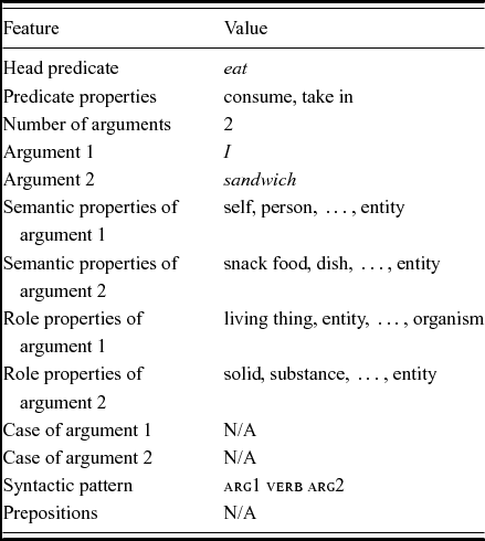
The exposure consists of a number of argument structure instances (AS instances) represented as assemblies of different information cues (or features). Each instance corresponds to an individual verb usage: an utterance and the respective perceptual context. A sample verb usage and its corresponding AS instance are presented in Table 1. The features include the head predicate (verb) and its semantic properties (lexical meaning), the number of arguments that the verb takes, argument heads, their cases, their semantic and event-based (thematic role) properties, prepositions and the syntactic pattern (which reflects the word order and the presence or absence of prepositions at specific slots). Instead of representing lexical meanings or thematic roles symbolically, we use a set of elements for each of these, following the theories of Dowty (Reference Dowty1991), and McRae, Ferretti and Amyote (Reference McRae, Ferretti and Amyote1997). Composite representations allow the model to estimate the similarity between different meanings or thematic roles. Sets of elements may be rather large: therefore for brevity we only show three elements for each feature in Table 1. Unlike semantic and role properties, some other features, for example head predicate and prepositions, take language-specific values. When a feature such as argument case is absent in a language (e.g., English), it is assigned a dummy value (ɴ/ᴀ). Note that the cases are the only morphological features in our setup, other morphological elements as well as articles are ignored, as they contribute little to differentiating between argument structure constructions.
An example AS instance extracted from a verb usage I ate a tuna sandwich.

Learning process
The learner maintains a set of constructions, which are represented as generalizations over AS instances. More specifically, each construction is an assembly of feature values of all instances that the model has decided to add to this construction. The learner tracks the frequency of each construction (the number of participating instances), together with the frequencies of all feature values, yet the original instances are not recoverable. The learner receives one instance at a time and iterates over all the acquired constructions, to find the one that can best accommodate the new instance. Two factors determine which construction the new instance is added to:
-
1. The frequency of each construction in the previously encountered input. This follows the idea in usage-based linguistics that linguistic units become entrenched through their use (e.g., Langacker, Reference Langacker1987; Schmid, Reference Schmid, Geeraerts and Cuyckens2007; MacWhinney, Reference MacWhinney, Gass and Mackey2012). A construction which already contains a large number of instances is more entrenched, or more readily accessible, therefore the learner is more likely to add the new instance to this construction. Note that this is to a certain extent similar to processing limitations that arise in connectionist models at later stages of learning (e.g., Ellis & Lambon Ralph, Reference Ellis and Lambon Ralph2000). However, the maximal processing capacity of our model (the number of categories) is not predefined as is the number of units in connectionist models, and we make no claims regarding how similar the two approaches are.
-
2. The similarity between the new AS instance and each construction, which is measured in terms of each feature independently (see Table 1 above). For example, if a construction and the new instance share the number of arguments, the syntactic pattern and the argument role properties, it is likely that this instance belongs to this construction. Vice versa, if a construction and the new instance have little in common in terms of feature values, the new instance is unlikely to be added to this construction. This similarity-based learning mechanism comes from the original model in Anderson (Reference Anderson1991) and reflects the role of similarity in human categorization (e.g., Sloutsky, Reference Sloutsky2003; Hahn & Ramscar, Reference Hahn, Ramscar, Hahn and Ramscar2001).
Upon estimating the two values, the learner adds the new AS instance into one of the constructions. However, especially at the beginning of the learning process, the best decision (as informed by the likelihood values) may be to create a new construction and add the new instance to this new construction (which would be identical to the instance). This happens when the new instance is very dissimilar to all the constructions the learner has acquired so far.Footnote 1
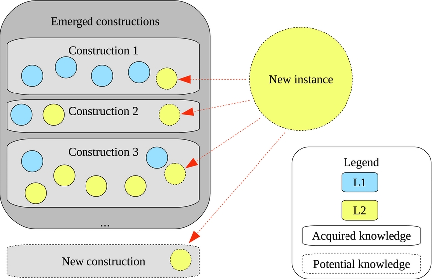
Exactly the same algorithm applies to L1 and L2 learning, as illustrated by Figure 1. Note that constructions may contain instances from only L1 or L2, as well as from both languages. Although such features as head predicate, arguments, and prepositions contain implicit information about the language of each AS instance, the model is not explicitly enforced to distinguish between the two languages. It is the input data and the probabilistic learning mechanism that determine to what extent L1 and L2 share their ‘storage resource’.
Deciding on a construction for a newly encountered L2 AS instance.

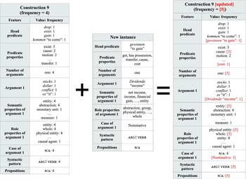
We further illustrate the learning process in Figure 2, where an English speaker learning L2 German encounters an AS instance with the head predicate gewinnen “to gain”. Note that construction 9 is associated, among other English verbs, with gain, and the instance headed by gain shares some feature values with the new instance headed by gewinnen. Thus, among all the existing constructions, construction 9 may be the most likely candidate for adding the new AS instance. Imagine, however, that the learner, upon receiving a substantial amount of English input, encounters a German instance with a syntactic pattern ᴘʀᴇᴘ ᴀʀɢ1 ᴠᴇʀʙ ᴀʀɢ2 ᴀʀɢ3 (e.g., Über die Nebenwirkungen weiß niemand das geringste. “No one knows anything about the side effects.”). This order of arguments is not typical for English, therefore the learner might not know a suitable construction to accommodate this AS instance, and is likely to create a new construction for the novel instance.
Updating a construction with a newly encountered AS instance. The frequency of the construction represents the number of AS instances it is based on. The frequency of each feature value equals to the number of participating AS instances showing this value for the respective feature. Square brackets denote updated elements.

Simplifying assumptions
Like all computational models in the field, our model simulates only certain aspects of learning, and makes a number of simplifying assumptions about the other aspects. Because we focus on the learning of abstract constructions, we assume that our simulated learner is able to segment the utterance and recognize all the words; it knows the meaning of most words in the utterance; it can identify the role of each participant in a given perceptual context; and it is able to infer the information about linguistic cases in the utterance. For the purpose of this study, we assume that the learning mechanism has acquired these types of knowledge and abilities by the moment it starts learning constructions, although we acknowledge that human learners acquire different types of knowledge in parallel (see, e.g., Lieven & Tomasello, Reference Lieven, Tomasello, Robinson and Ellis2008, for child learning).
Testing L2 proficiency
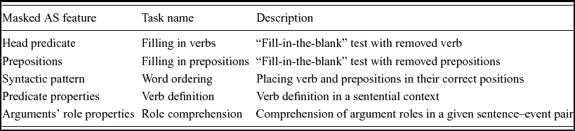
The model's knowledge of argument structure constructions is tested in terms of the accuracy of language use, both in production and comprehension. A formal description of the testing method is provided in Appendix A, while here we outline the general approach to testing and focus on the actual tasks. We use five tasks for evaluating the model, each of them testing a different aspect (or feature) of the model's construction knowledge. We provide the model with a number of test instances in which the values of some features are masked. Although it is possible to mask the values of multiple features at once, each of the tasks in this study masks only a single feature. Thus, for each test instance, the model has to predict the missing value of a particular feature given the values of the other features. The prediction accuracy in each task is estimated based on the match between the original (masked) value and the value predicted by the model.
Such approach relates to the view in usage-based linguistics that linguistic knowledge is reflected in language use. Although the main motivation for the task choice comes from the model architecture, the tasks we employ map onto some existing methodologies used either in L2 assessment or in experimental studies with children and adults (see Table 2). Note, however, that our test tasks are conceptually closer to spontaneous language use rather than to traditional language assessment,Footnote 2 therefore the examples (1)–(5) below are provided mostly for illustrative purposes, while the actual testing algorithm can be found in Appendix A.
Assessment tasks with their descriptions and corresponding features in AS instances.

Filling in verbs
In this task we elicit the production of verbs that the model finds suitable in a given test instance. This is close to the method used in some experimental studies concerned with the learning of argument structure constructions, as they tend to examine the distribution of verbs in specific constructions (e.g., Ellis et al., Reference Ellis, O'Donnell and Römer2014; Gries & Wulff, Reference Gries and Wulff2005):
-
(1) Fill in a verb: I _____ a sandwich.
Filling in prepositions
The same design is used to elicit the production of prepositions. Filling in blank slots with missing prepositions is a classic task in L2 assessment (e.g., Oller & Inal, Reference Oller and Inal1971):
-
(2) Fill in a preposition: John gave an apple _____ Mary.
Word ordering
Given the verb and its arguments, the task is to name a matching syntactic pattern. This is similar to a common L2 assessment task in which learners are asked to unscramble the words into a grammatical sentence (e.g., Wesche & Paribakht, Reference Wesche and Paribakht2000):
-
(3) Arrange the words to form a grammatical sentence: ate, (a) sandwich, I.
Verb definition
The task of deriving lexical meanings from contexts tests learners’ ability to comprehend verbs. A similar definition task has been used, for example, for assessing children's vocabulary (Cain, Reference Cain2007). A schematic example for our setup is given in (4):
-
(4) Describe the lexical meaning of ate in the sentence: I ate a sandwich.
Role comprehension
Studies in which humans have to learn new verbs (e.g., Akhtar & Tomasello, Reference Akhtar and Tomasello1997; Wonnacott, Newport & Tanenhaus, Reference Wonnacott, Newport and Tanenhaus2008) often test the acquisition of verb-general knowledge about the thematic roles of participants in a given event. Similarly, our model is required to describe the role of each participant in a given sentence–event pair:
-
(5) Describe the thematic roles of I and (a) sandwich in the sentence: I ate a sandwich.
Input and test instances
In preliminary experiments (Matusevych, Alishahi & Backus, Reference Matusevych, Alishahi, Backus, Demberg and Levi2013) we tested the model on small data sets of German and English, in which argument structures were annotated manually. However, manual annotation of larger data sets would be very time-consuming. Instead, in the present study we extracted data from available annotated resources for the same languages. Essentially, the data come from German and English newspaper texts. Although these texts do not represent the kind of language that L1 and most L2 learners are exposed to, we used these corpora as the only large sources of English and German that contained all the necessary types of annotations related to argument structure.
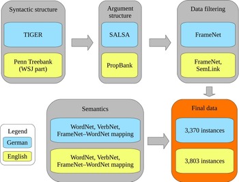
Figure 3 schematically shows the resources we used and the steps we took for preparing the input data. The syntactically annotated data originate from the TIGER corpus for German (Brants, Dipper, Eisenberg, Hansen-Schirra, König, Lezius, Rohrer, Smith & Uszkoreit, Reference Brants, Dipper, Eisenberg, Hansen-Schirra, König, Lezius, Rohrer, Smith and Uszkoreit2004) and the Penn Treebank for English (Marcus, Kim, Marcinkiewicz, MacIntyre, Bies, Ferguson, Katz & Schasberger, Reference Marcus, Kim, Marcinkiewicz, MacIntyre, Bies, Ferguson, Katz, Schasberger and Weinstein1994). The German SALSA corpus (Burchardt, Erk, Frank, Kowalski, Padó & Pinkal, Reference Burchardt, Erk, Frank, Kowalski, Padó, Pinkal, Calzolari, Choukri, Gangemi, Maegaard, Mariani, Odijk and Tapias2006) and English PropBank (Palmer, Gildea & Kingsbury, Reference Palmer, Gildea and Kingsbury2005) contained the types of annotations that helped us to extract argument structure from sentences. Further, for consistency between the languages, we filtered the resulting sentences and kept only those that were annotated with FrameNet frames (see Ruppenhofer, Ellsworth, Petruck, Johnson & Scheffczyk, Reference Ruppenhofer, Ellsworth, Petruck, Johnson and Scheffczyk2010). While some German data were already annotated so in SALSA, for English we had to use the mappings between PropBank and FrameNet, provided in SemLink (Palmer, Reference Palmer, Rumshisky and Calzolari2009). Finally, semantic features for individual lexemes were extracted from WordNet (Miller, Reference Miller1995) and VerbNet (Schuler, Reference Schuler2006). The existing mappings between WordNet and FrameNet (Bryl, Tonelli, Giuliano & Serafini, Reference Bryl, Tonelli, Giuliano, Serafini, Ossowski and Lecca2012) also made it possible to automatically expand argument thematic roles into sets of elements. The procedure resulted in German and English data sets containing 3,370 and 3,803 AS instances, respectively. Note that the two data sets have similar, but not identical sizes. Besides, they may differ in the amount of noise originating from either the corpus annotations or from our data extraction procedures. This potentially may result in one of the data sets being more difficult to learn than the other.
Schematic representation of the input data preparation.

Importantly, a substantial part of both German and English AS instances originated from embedded clauses. While in English main and embedded clauses have analogous word order, this is not so for German, where embedded clauses are usually verb-final. Consider the following English sentence (6) translated into German (7):
-
(6) The group said (that) it sold the shares.
-
(7) Die Gruppe sagte, dass sie die Aktien verkauften.
The word order in the English embedded clause in (6) is SVO, while the German order (7) is SOV. This is a natural difference if one considers each complex sentence as a whole. However, we represent each AS as an independent language unit, and the unnaturally large number of SOV sentences would make our data set a non-representative sample of German (simple) sentences. Ultimately, this would provide our model with an unrealistic tool to distinguish between English and German syntactic structures. Therefore, we ‘recovered’ German verb-second word order in embedded clauses by manually assigning the second position to the verb. Note, however, that the order of arguments was never changed, so that the data contained both SVO and OVS sentences.
From the resulting data sets, input to the model was sampled randomly, so each individual simulation represented a learner with a unique history of language exposure. Thereby, in our experiments we sometimes refer to different simulations as individual learners. The exact number of German and English AS instances as well as the temporal pattern of their presentation were determined by the experimental setup, however all the experiments were run twice – using German as L1 and English as L2, and vice versa.
Similarly, test instances are randomly sampled from the data. Learners are tested on different test sets, although every learner is repeatedly offered the same test set at certain intervals. Furthermore, each learner performs most language tasks on a single test set, except for the task of filling in prepositions, for which an additional test set is prepared. This is because most AS instances in our data (approximately 70% for German and 90% for English) contain no prepositions, and sampling items randomly would result in having no prepositions in the majority of test instances. Therefore, we sample an additional test set for each learner, considering only instances with prepositions. Just as in human language learning, some test items may be identical to input items that the model has encountered. In other words, sampling the input and the test instances from the same data resembles better a natural language learning setting than splitting the data into a train and a test set (a common practice in computational linguistics). It is unlikely that the model can memorize specific instances and then simply reproduce them, because construction learning is implemented as a categorization task, without memorizing actual instances. However, to ensure that the model does not memorize the exact instances, we run an additional set of simulations, in which none of the learning data appear as test instances.Footnote 3 The described data is used in all the experiments that we report in the next section.
Experiments and results
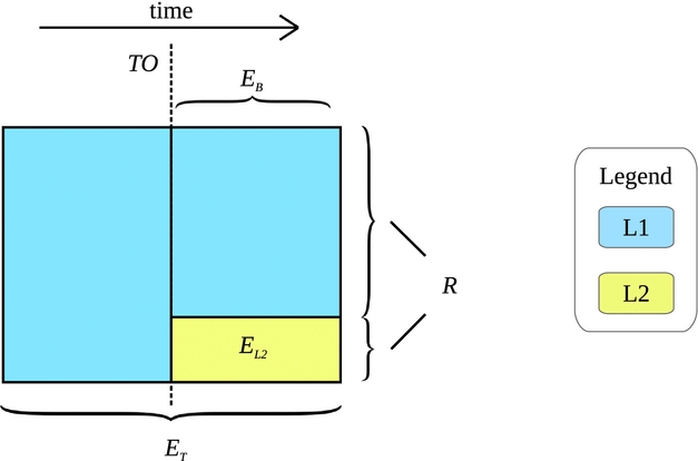
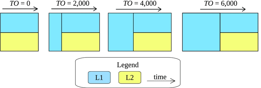
This section describes the design and the results of three experiments. The first two are intended to test whether the general learning principle “the more, the better” holds for statistical learning of argument structure constructions – that is, whether the larger amount of L2 input results in higher L2 performance. We measure L2 amount both in relative (experiment 1) and absolute terms (experiment 2). Experiment 3 is designed to test how learners’ L2 performance is affected by the time of L2 onset. In all the experiments, we quantify various amounts of input in terms of the respective number of AS instances. Furthermore, we adopt the following notations (see Figure 4):
-
1. ET – total language exposure, both L1 and L2. E.g., ET = 12,000 AS instances.
-
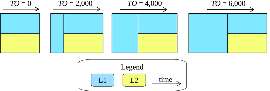
2. TO – the time of onset, expressed as the amount of L1 input prior to the L2 onset. E.g., TO = 9,000 L1 instances. TO = 0 defines a simultaneous bilingual.
-
3. EL2 – cumulative L2 exposure in absolute terms. E.g., EL2 = 3,000 L2 instances.
-
4. R – the ratio of L1 amount to L2 amount at each interval after TO. E.g., R = 20:1 means that the learner receives 20 times more L1 input than L2 input.
-
5. EB – the amount of bilingual input, in which both L1 and L2 instances are present. E.g., EB = 6,000 indicates that after TO, the learner receives 6,000 instances of bilingual input, where L1 and L2 are mixed in the proportion determined by R.
Notations used in the experiments.

Amount of L2 input
Experiment 1
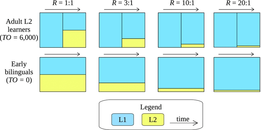
In this experiment learners’ exposure to L2 was measured in relation to their L1 exposure. To investigate whether the relative amount of L2 input would affect learners’ L2 performance, we manipulated the ratio R in four groups of simulated learners, while keeping ET constant. The first group of learners received equal amounts of L1 and L2 input at each learning interval after L2 onset, R = 1:1, while for the other groups R was set to 3:1, 10:1, or 20:1, respectively. Such design simulated a common SLA setting: adult L2 learners are often exposed to the target language in small quantities, while L1 still dominates in their daily use. Each of the four groups consisted of 30 learners, for which both TO and EB were set to 6,000 instances – to simulate a population of adult L2 learners. Our choice of the TO value 6,000 was justified in our preliminary simulations, which had shown that after encountering approximately 6,000 AS instances learners’ L1 performance stabilized (although not completely, and this differed somewhat depending on the task). This way, ET = TO + EB = 12,000. Similarly, we simulated four more groups of early bilinguals (TO = 0, ET = EB = 6,000) with different R values (see Figure 5).
The setup of experiment 1. Two rows show the population types, four columns show the learner groups.

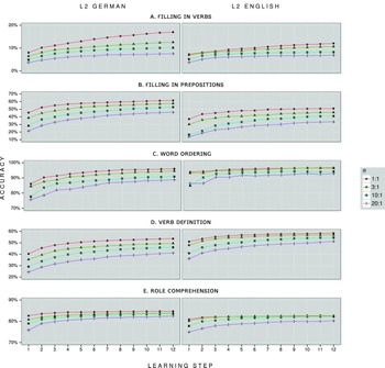
After every 500 input instances, learners’ L2 proficiency was tested using the five tasks described in the previous section. Figure 6 shows the average performance curves for each of the four groups of adult learners.
Average learning curves for adult learners with different R values, ET is kept constant.

First, we notice that in most tasks the performance curve flattens far below 100%. This is partly because all the tasks underestimate learners’ L2 knowledge: while each test item assumes a single ‘correct’ answer, there may be more than one acceptable answer. When filling in verbs, for example, some empty slots may fit several semantically related verbs – synonyms (8) or antonyms (9).
-
(8) He acquired (bought) 300,000 shares of the stock.
-
(9) Industrial output fell (rose) 0.1% in September.
The size of the described effect is different for each task, which contributes to the different learners’ performance across tasks (note that in Figure 6 the tasks are plotted on different scales). Additionally, there are certain differences between the model's performance in L2 German and L2 English tasks (compare the plots in Figure 6 pairwise). We explain this by possible differences in complexity between the German and English data sets, which we mentioned in the subsection Input and test instances above.
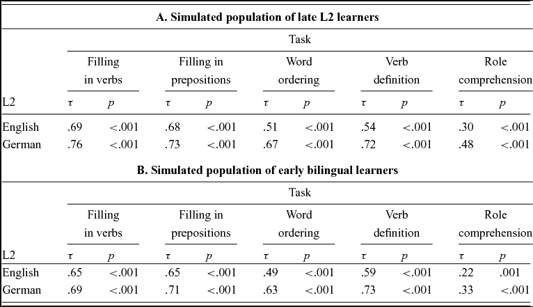
Despite the differences between the tasks, each individual plot in Figure 6 reveals the same pattern. Higher relative amount of L2 input corresponds to better L2 performance at each point in time. To statistically test whether the relative amount of L2 input correlated with the L2 performance at the end of learning, we ran Kendall's tau correlation testsFootnote 4 (see Table 3A). The results revealed a highly significant correlation between the amount of L2 input and the performance in each task in late learners, both for L2 English and L2 German. The results for early bilinguals yielded very similar patterns, thus we do not provide the plots of their learning curves, however the results of the correlation tests are shown in Table 3B.
Results of correlation tests between R and L2 performance at the end of learning, ET is kept constant.

The results in Table 3 suggest that receiving more L2 input (in relation to L1 input) by a statistical learner leads to the better knowledge of L2 argument structure constructions. This may be due to the interaction of L2 input with the ongoing exposure to L1 input. However, so far we have assumed that learners’ performance achieves its maximum at the end of learning simulations (upon receiving 6,000 mixed AS instances). This may be the case for the easier tasks, but the more difficult ones may take learners more time to achieve the highest possible performance, especially in case their cumulative EL2 is low because of a high R value (e.g., 20:1). For example, most learning curves for filling in verbs (see Figure 6A) do not flatten at step 12. Thus, it may be the case that learners in each group could potentially achieve the same performance, irrespective of the R value, if only they had enough time to learn. In this interpretation the L2 attainment depends not on the relative, but on the absolute amount of L2 input. To test whether this would be true, we ran another experiment.
Experiment 2
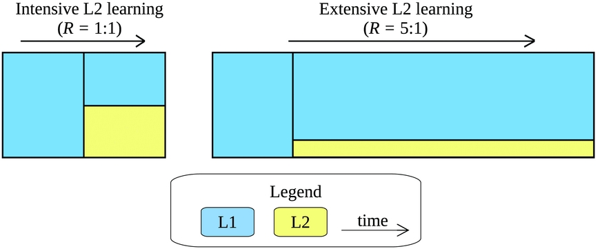
The setup of this experiment was similar to that of experiment 1, however this time we kept the absolute amount of L2 input constant (EL2 = 1,500), while manipulating R. The latter was set to 1:1 (intensive L2 learning) or 5:1 (extensive L2 learning) – see Figure 7 (note that the length of L2 exposure is different in the two conditions, but the total L2 area is identical). Since the results of experiment 1 did not differ substantially for early bilinguals and adult learners, this time we simulated only the latter population by setting TO to 6,000.
The setup of experiment 2.

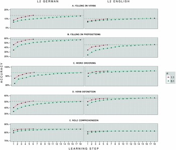
If the relative amount of L2, indeed, determines the level of L2 attainment in a statistical learner, then we expect the performance to differ in the two groups. However, if it is only the absolute amount of L2 input that matters, there must be no difference in proficiency between the two conditions. The learning curves are shown in Figure 8.
Average learning curves for learners with different R values, EL2 is kept constant.

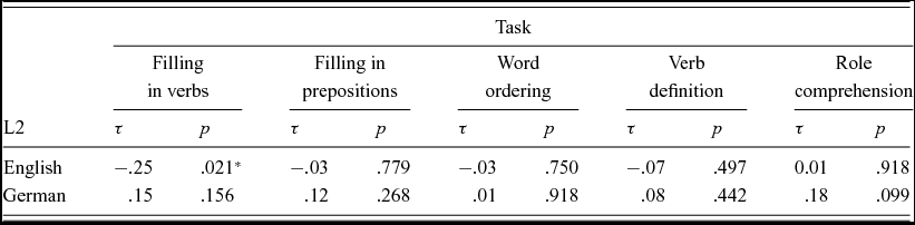
Each individual plot in Figure 8 shows that the learner ultimately achieves the same or very similar performance in both conditions. In case of intensive learning, the curve is steep and reaches the highest level fast, while in the extensive condition learning goes much slower. The final performance is comparable, however: see the horizontal lines in Figure 8. Again, we ran Kendall's tau correlation tests using the final performance values. Table 4 shows the results of these tests.
Results of correlation tests between R and L2 performance at the end of learning, EL2 is kept constant.

The results show no significant correlations between R and learners’ final performance for most tasks, the correlation reaching significance only for filling in verbs in L2 English: τ = −.25, p = .021. Since the correlation is negative, learners’ performance in this task is higher in the extensive condition (R = 5:1) than in the intensive condition (R = 1:1). We believe this reflects learners’ ongoing enhancement of L1 verbs. As we mentioned, filling in verbs is the most difficult task of the five, therefore continuing L1 exposure after TO aids learners in memorizing some contexts in which L1 verbs are used. As the extensive condition exposes learners to more L1 input than the intensive condition, they memorize more of these contexts, which helps them in discriminating between L1 and L2 contexts. As a result, at the end of learning in the extensive condition the model produces fewer L1 instances than in the intensive condition, hence the higher performance.
For the other tasks only the absolute amount of L2 input determines the resulting knowledge of L2 argument structure constructions. This suggests that length of exposure makes no difference, as long as the cumulative amount of L2 input stays the same.
Time of L2 onset
Experiment 3
This experiment was designed to investigate whether learners’ L2 performance could be influenced by the time of L2 onset. If constructions and words are learned in a similar manner, then a negative effect of higher L1 entrenchment is to be expected (e.g., MacWhinney, Reference MacWhinney, Gass and Mackey2012). Later L2 onset would lead to higher L1 entrenchment and, because of the interference this entails, lower L2 proficiency.
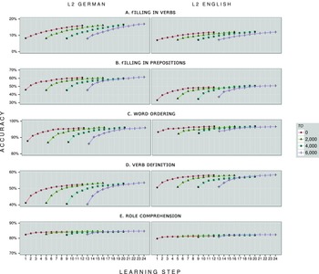
We manipulated the prior amount of L1 input by setting TO to 0 (simultaneous bilinguals), 2,000, 4,000 or 6,000 (late L2 learners). As we mentioned, in our preliminary simulations the maximum L1 performance was achieved only after approximately 6,000 AS instances, thereby we chose TO values under 6,000 to ensure that the level of L1 entrenchment is different for each TO. For all the four groups of learners, EB was set to 6,000, and R was equal for all the groups (1:1), therefore EL2 amounted to 3,000 instances for each learner. The only difference between the groups, then, was the TO value. The experimental setup is shown in Figure 9, while Figure 10 illustrates the average learning curves for each group.
The setup of experiment 3.
Average learning curves for learners with different TO values.

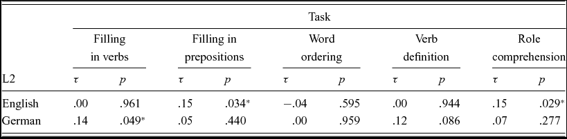
If we look at each individual plot, we can notice no obvious pattern of difference between the four groups – in each case the learning curves seem to reach similar accuracy values. To statistically test whether learners’ resulting performance at the end of learning correlated with TO, we ran Kendall's tau correlation tests (see Table 5).
Results of correlation tests between TO and L2 performance at the end of learning.

The results suggest that the time of L2 onset does not affect the simulated learners’ performance at the end of learning, with some exceptions. We do observe significant positive correlations between TO and the ultimate L2 performance for two tasks in L2 English (filling in prepositions and role comprehension), and a marginally significant correlation for filling in verbs in L2 German. Note that the correlations are positive, meaning that later TO leads to better L2 performance. This suggests a positive impact of cross-linguistic transfer from L1 to L2. English and German argument structures have a lot in common, as the two languages are typologically close: they both have SVO order in main clauses, and both are satellite-framed. Thus, the model may use the existing L1 knowledge to perform better in L2 tasks. The higher L1 entrenchment at TO is, therefore, beneficial, and may well give the model a small long-term advantage in L2 performance.
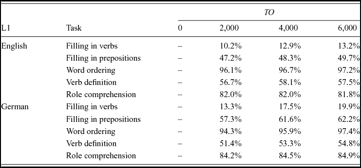
Most correlations in Table 5, however, are not significant. To ensure this is not caused by the similar degree of L1 entrenchment at TO in some groups (with TO = 2,000, TO = 4,000, and TO = 6,000), we compared the average L1 performance at TO in the three mentioned groups. Table 6 shows that L1 performance in the three groups differs in most tasks. The only deviation from this pattern is observed for role comprehension in L1 English, where the L1 performance of the three groups is approximately equal. This, in fact, makes our correlation result for role comprehension in L2 German non-informative, because the difference in ultimate L2 performance is not to be expected for the three groups with equal degree of L1 entrenchment at TO.
Average L1 performance at TO in different learner groups in experiment 3.

Before drawing any conclusions regarding the effect of the time of onset, we should additionally look at whether such effect is present at the earlier learning stages as well, since the presented correlation results are estimated for the learners’ performance at the end of learning only. In addition, the correlation results do not tell us whether the time of onset interacts in any way with learners’ cumulative amount of L2 exposure. To test this, we ran a series of regression models that predicted learners’ performance at each learning stage.
L2 performance: contributions of individual factors
Regression models were used to examine the potential effects of TO, EL2 , and their interaction. Conceptually speaking, we checked whether at any learning stage learners’ L2 performance in a certain task could be predicted by TO and EL2 . We ran ten linear mixed effects models (Baayen, Reference Baayen2008), one for each task in each language, using the lme4 package for R (Bates, Mächler, Bolker & Walker, n.d.). To account for possible individual variation between learners, we introduced a random factor of learner. Each model had the maximal random effect structure justified by the data sample (Barr, Levy, Scheepers & Tilly, Reference Barr, Levy, Scheepers and Tilly2013), slightly varying for different tasks and languages due to convergence issues.
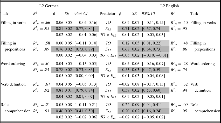
All the models were run on the learning results reported on for experiment 3. Recall that in experiment 3 we manipulated TO, but not EL2 . Nevertheless, the latter was present in the learning results of our simulations, because we tested the model's performance at different learning stages (that is, after it was exposed to different amounts of L2). Therefore, each performance score had an EL2 value associated with it, which we used in the regression. This setup implies that the regression models do not only provide results in terms of ultimate L2 proficiency (as did the correlation tests reported in the previous sections), but at each moment of learning. Importantly, L2 performance is not a linear function of EL2 in our experiments (recall the shapes of the learning curves). In general, learning success is believed to be a power function of experience (Newell & Rosenbloom, Reference Newell, Rosenbloom and Anderson1981). To account for this relation between performance and EL2 , we log-transformed all the performance values and EL2 , but also TO for consistency. To eliminate the problems of multicollinearity and variance inflation, and to make the regression coefficients directly comparable, we standardized all the variables. A summary of the models is given in Table 7.
Summary of mixed effects models predicting learners’ L2 performance (predictors names are given in the central column).

Note: R2 m and R2 c stand for marginal and conditional R2 coefficients and indicate the amount of variance explained by the fixed factors and by the full model, respectively (Johnson, Reference Johnson2014). The reported SE and confidence interval values are estimated via parametric bootstrap with 1,000 resamples (Bates et al., n.d.).
L2 amount
The effect of EL2 is the only main effect observed for all the tasks in both German and English (see the dark gray cells in Table 7). As expected, the effect is always positive: learners’ L2 proficiency increases as they are being exposed to more L2 input. This supports the correlation between EL2 and learners’ L2 performance, found in experiment 1. Note that the standardized regression coefficients (β) for EL2 have the largest values, compared to the coefficients of TO and TO × EL2 in each regression model, which means that the effect of EL2 is stronger than that of TO and of the interaction. The only exception is role comprehension in L2 English, for which the coefficient of EL2 (0.20) is smaller than that of TO (0.22). Yet, the amount of variance explained by the fixed effects (R2 m ) in the respective regression model is the smallest (R2 m = .09, or 9%), compared to the respective value in all the other models (e.g., R2 m = .67 for verb definition in L2 German). The poor model fit suggests that the β coefficients in the regression model for role comprehension in L2 English might not be informative.
L2 onset
The main effect of TO is present only for L2 English and only for two tasks: filling in prepositions and role comprehension. This is comparable to the results of experiment 3, in which the correlation of TO with learners’ final L2 performance was observed for the same two tasks in L2 English. Additionally, in experiment 3 the same positive correlation was observed for a single task in L2 German (filling in verbs), but this was only marginally significant and is not supported by the regression results. As for the other two tasks with a main effect of TO, the analysis for role comprehension, as we mentioned, is not informative due to the poor model fit. This is not the case, however, for filling in prepositions. The impact of TO is positive: late L2 starters perform better than early L2 starters. This could be explained by the positive effect of cross-linguistic transfer. As we mentioned, the model may use the existing L1 knowledge to perform better in L2 tasks, and the higher level of L1 entrenchment is beneficial, especially at the early stages of L2 learning. Indeed, although the effect of transfer can be both positive and negative, the positive effect must prevail here due to the similarity of English and German argument structure constructions. However, the effect can be manifested differently in each of the five tasks used, due to their nature. Since the two languages in our model use shared representations of lexical semantics, participant roles, and word order, in such tasks as verb definition, role comprehension and word ordering, one would expect a positive transfer effect. For example, a simulated learner of L2 English may be able to describe the meaning of a novel English verb to increase, because it shares many contexts of use with its German translation steigen. This is different for the other two tasks – filling in verbs and prepositions. Since learners are allowed to use their L1 in the two “fill-in-the-blank” tasks, they are likely to produce L1 verbs and prepositions (which are different in German and English), hence the negative effect of transfer.Footnote 5 Note, however, that both German and English have a preposition in, often used in equal or very similar contexts. In our German data set, in is the most frequent preposition, which promotes its use by L1 German speakers during the testing in L2 English. Although the learners, in fact, use the German preposition, it may fit many English test instances that require the use of English in, hence the positive effect of lexical transfer from German to English. The same effect from English to German may not be observed, since in our English data set in is only the third most frequent preposition. Therefore, learners would more likely use the two more frequent prepositions (to and on) during the testing.
Interaction term
First we note that the interaction effect of EL2 and TO is significant for filling in prepositions in L2 English, with a negative β coefficient. Considering the positive effect of TO in this task we just discussed, this negative interaction can be interpreted as a decrease in the positive TO effect at the later stages of L2 testing. This supports our explanation of the positive TO effect in terms of positive transfer: higher L1 entrenchment is beneficial at the early stages of L2 learning, however at the later stages this benefit diminishes, because learners rely more on their acquired L2 knowledge than on L1 knowledge.
Finally, there is a significant interaction effect in verb definition in L2 German. The respective β coefficient is positive – that is, the positive effect of higher EL2 on learners’ performance is stronger for learners with later TO. In other words, in this task late L2 starters achieve a certain level of performance faster than early L2 starters. This observation also suggests that transfer has more positive than negative effect in verb definition in L2 German.
Discussion
In the present study we investigated how the learning of argument structure constructions in L2 was affected by two variables – the amount of L2 input (both relative and absolute) and the time of L2 onset. For this purpose, we computationally simulated the process of statistical construction learning in two languages and ran three experiments to test the performance of simulated learners under different conditions of exposure.
Amount of L2 input
The first variable, the amount of L2 input, affected learners’ L2 performance as expected – getting more L2 input resulted in better L2 performance. This is in line with a general learning rule “the more, the better”, which has been demonstrated to apply to human learners for various domains (e.g., Flege, Yeni-Komshian & Liu, Reference Flege, Yeni-Komshian and Liu1999; Muñoz, Reference Muñoz2011). In experiment 1, we captured this type of relation using a relative measure of L2 amount, while controlling for the length of L2 exposure. However, when the cumulative amount of L2 was kept constant instead (experiment 2), the model's performance appeared to be the same for varying relative amounts of L2. Intuitively, this is contrary to a well-researched spacing effect: spaced, or distributed, practice leads to higher test performance than massed practice in many domains (Küpper-Tetzel, Reference Küpper-Tetzel2014), including construction learning (Ambridge, Theakston, Lieven & Tomasello, Reference Ambridge, Theakston, Lieven and Tomasello2006). However, it has been argued (e.g., Cepeda, Pashler, Vul, Wixted & Rohrer, Reference Cepeda, Pashler, Vul, Wixted and Rohrer2006) that the learning depends not only on the length of the interstudy interval (the time between two presentations of an item), but also on that of the retention interval (the time between its last presentation and the test). Thus, simulations with a systematic control of the two intervals (with respect to the presentation of individual L2 instances) are needed to relate our findings to the existing research in this domain.
In the current study we focused only on the quantitative characteristics of L2 input, but the quality of L2 input may be equally important (Moyer, Reference Moyer2005). Obviously, it cannot be the mere amount of input that determines learners’ L2 proficiency, as an identical amount of input may be very different for two different learners, in terms of relevance for the learner, grammatical complexity, lexical diversity, native-likeness, discourse style, etc. All these characteristics contribute to learners’ level of engagement with the target language and affect the learning process. Therefore, an ideal measure of L2 input should account for much more than its overall amount. Preliminary versions of such measures have already been proposed, but they need further refinement. For example, Ågren, Granfeldt and Thomas (Reference Ågren, Granfeldt and Thomas2014) have developed an individual input profile score, yet they recognize it does not take into account that different input domains may affect the learning to a different degree.
Time of L2 onset
The second variable that we investigated – the time of L2 onset – appeared not to have any impact on performance in most L2 tasks. The only exceptions were two tasks in L2 English – filling in prepositions and role comprehension, where later L2 starters performed better than early starters. The latter exception, as we showed, could be due to the poor fit of the respective regression model. As for filling in prepositions, later L2 starters had a better knowledge of a frequent German preposition in, and they could transfer this knowledge into L2 to identify the correct contexts of use of the English preposition in. Overall, unlike in other linguistic domains such as lexis and morphology (Zhao & Li, Reference Zhao and Li2010; Monner et al., Reference Monner, Vatz, Morini, Hwang and DeKeyser2013), a pronounced negative effect of L1 entrenchment (i.e., later L2 onset) on learning L2 argument structure constructions is absent in our experiments. The difference between the domains relates to a discussion in literature on L1 processing or, more broadly, on the age/order effect. It has been shown (Lambon Ralph & Ehsan, Reference Lambon Ralph and Ehsan2006) that the negative effect of a later acquisition of a specific item (e.g., word) in cued production is higher for stimuli with more arbitrary cue–outcome mappings (e.g., word phonology and meaning), and lower for stimuli with more consistent mappings (e.g., word phonology and orthography). In case of arbitrary mappings, the meaning of a novel word can hardly be predicted from its phonological form, despite a potentially large number of earlier acquired mappings. On the contrary, word orthography is often predictable from its phonological form, due to the consistency of the mapping with earlier acquired words. In the context of bilingual learning we look at the consistency of mappings across L1 and L2, rather than across multiple L1 items. In our test tasks each cue (i.e., test AS instance) consisted of multiple features, and the model, in fact, could predict the outcome (i.e., the value of the missing feature) based on the mappings between the features in L1: the languages we used in this study – German and English – were typologically close, and positive transfer was likely to take place. This could be the reason why the negative effect of the late onset was not observed.
In the light of the ongoing discussion about the age/order effect in literature, we can further note that our results do not support the idea proposed by Stewart and Ellis (Reference Stewart and Ellis2008) that the age/order effect is a property of any learning system. Instead, our findings are consistent with the cumulative frequency hypothesis (Lewis et al., Reference Lewis, Gerhand and Ellis2001; Zevin & Seidenberg, Reference Zevin and Seidenberg2002), which claims that the accessibility of a word is determined by its cumulative frequency, but not the moment of its first encounter.
Due to the lack of available annotated resources we only used English and German in the current study. We plan to explore new resources and investigate the bilingual learning of argument structure constructions in additional language pairs, to determine the exact contribution of cross-linguistic transfer effects to such learning. The computational tool used for our study focuses on only a subset of (input-related) factors and is not meant to represent the whole picture of how humans learn a second language. Nevertheless, it has provided rather robust and consistent results by allowing for full control of the variable confounding and of the input quantities, which cannot be easily done in human subject studies. These advantages make the presented model a promising tool for future studies.
Appendix A. Formal model
Basic notations
In this appendix, the following notations are used: C – a construction; I – an argument structure instance, S – the feature set used by the model. The feature set consists of a number of features F k :
 $$\begin{equation}
{S = \left\{ {{F_{\rm{1}}},{F_{\rm{2}}},{F_{\rm{3}}}...,{F_n}} \right\}}\end{equation}$$
Each featureF k ∈ S is represented by multiple values in a data set, which we denote using the feature cardinality |F(k)|. Some features by definition take single string values, while other features are defined as sets of elements, e.g.:
 $$\begin{equation}
{{F_k} = \left\{ {abandon,about,accept...,wrong} \right\}}
\end{equation}$$
An instance I is, in fact, a unique combination of specific values (FI k ) of all features F k ∈ S:
 $$\begin{equation}
{I = \left\{ {F_{\rm{1}}^I,F_{\rm{2}}^I,F_{\rm{3}}^I...,F_n^I} \right\}}
\end{equation}$$
Each construction C also has a combination of values (FC k ) of eachF k ∈ S associated with it. However, each element e ∈ FC k may occur inFC k multiple times. In other words,FC k is a multiset, and |ei | denotes the number of occurrences of ei inFC k .
Learning
The learner processes instances one by one: N denotes the number of instances encountered by a certain moment of time. For a given instance I, the model looks for the most probable construction Cbest :
 $$\begin{equation}
{C_{best}}(I) = \mathop {\arg \max }\limits_C P(C|I)
\end{equation}$$
In (4), C ranges over all the constructions learned so far, as well as a potential new construction. The conditional probability in (4) can be estimated using the Bayes rule:
 $$\begin{equation}
{P\left( {C|I} \right) = \frac{{P\left( C \right)P\left( {I|C} \right)}}{{P\left( I \right)}}}
\end{equation}$$
Since the denominator P(I) in (5) is the same for all constructions, it can be dropped when comparing the probabilities of constructions:
 $$\begin{equation}
{\frac{{P\left( C \right)P\left( {I|C} \right)}}{{P\left( I \right)}} \propto P\left( C \right)P\left( {I|C} \right)}
\end{equation}$$
In (6), there are two factors that determine which construction the new instance is added to: prior probabilityP(C) and conditional probabilityP(I|C). P(C) is proportional to the frequency of C in the previously encountered input – in other words, the number of instances that C contains:
 $$\begin{equation}
{P\left| C \right| = \frac{{\left| C \right|}}{{N + {\rm{1}}}}}
\end{equation}$$
For the potential (new) construction C 0 the frequency is initially assigned to 1, to avoid zero values in the multiplicative formula (6):
 $$\begin{equation}
{P\left( {{C_{\rm{0}}}} \right) = \frac{{\rm{1}}}{{N + {\rm{1}}}}}
\end{equation}$$
The conditional probability captures the similarity between the encountered instance I and a construction C. The features are assumed to be independent, and the overall similarity is a product of the similarities in terms of each feature. Considering (3), this can be noted as follows:
 $$\begin{equation}
{P\left( {I|C} \right) = \prod\limits_{k \in {\rm{1}}..n} P \left( {F_k^I|C} \right)}
\end{equation}$$
For features which take a single (string) value, such as the head verb, this probability is computed via a smoothed maximum likelihood estimator:
 $$\begin{equation}
{P\left( {F_k^I|C} \right) = \frac{{\left| {\{ F_k^I|F_k^I \in F_k^C\} } \right| + \lambda }}{{\left| {F_k^C} \right| + \lambda \left| {{F_k}} \right|}}}
\end{equation}$$
In (10), |{FI k |Fk I ∈ FC k }| denotes the number of occurrences of FI k in the multiset FC k , while λ is a smoothing parameter, whose value is set as described in the final section of this Appendix. Note that for a new construction |{FI k |Fk I ∈ FC k }| = |Fk C | = 0.
For features with a set value such as the semantic properties of the verb and the arguments, the method given in (10) is too strict, because any two sets of properties (e.g., lexical meaning properties) are unlikely to be fully identical, so that |{C|FC k = Fk I }| would always equal zero. Therefore, the conditional probability for each set feature is calculated as follows (cf. Alishahi & Pyykkönen, Reference Alishahi, Pyykkönen, Carlson, Hoelscher and Shipley2011):
 $$\begin{eqnarray}
{P\left( {F_k^I|C} \right) = \frac{{\rm{1}}}{{\left| {{F_k}} \right|}}\prod\limits_{e \in F_k^I} {P\left( {e|C} \right)} \times \prod\limits_{e \in {F_K}\backslash F_K^I} {P\left( {\neg e|C} \right)} }\nonumber\\
\end{eqnarray}$$
In (11), F
k
is the superset of all values of the respective feature in the data set. Then, Fk
\FI
k
denotes all potential elements in F
k
which do not occur inFI
k
. The probabilities P(e|C) and
 $P(\neg e|C)$
are computed as given in (10), to obtain the probability of each element e occurring or not occurring, respectively, in C.
Testing
At certain intervals, the language proficiency (L2 proficiency, in our case) of the model is tested on a number of test tasks. Each task contains in total T test instances. To create a test instance Itest , a value of a single feature F x in I is masked (FI x ), so that the resultingItest is incomplete:
 $$\begin{equation}
{{I_{test}} = I\backslash F_x^I}
\end{equation}$$
The model, then, has to predict all the values that could be used in place of FI x , and their probabilities, givenItest . We denote the enumerated set of predicted values as Fpredicted x . The probability of each Fj x ∈ Fx predicted is calculated as follows:
 $$\begin{equation}
{P\left( {F_x^j|{I_{test}}} \right) = \sum\limits_C P \left( {F_x^j|C} \right)P\left( {C|{I_{test}}} \right)}
\end{equation}$$
The right part in (13) is the sum over all acquired constructions.P(Fj x |C) is computed as given in (10), while P(C|Itest ), again, can be transformed using the Bayes rule:
 $$\begin{equation}
{P\left( {C|{I_{test}}} \right) = \frac{{P\left( C \right)P\left( {{I_{test}}|C} \right)}}{{P\left( {{I_{test}}} \right)}}}
\end{equation}$$
Dropping the constant denominator in (14) yields:
 $$\begin{equation}
{\frac{{P\left( C \right)P\left( {{I_{test}}|C} \right)}}{{P\left( {{I_{test}}} \right)}} \propto P\left( C \right)P\left( {{I_{test}}|C} \right)}
\end{equation}$$
The two probabilities in the right part of (15) are computed using equations (7) and (9), respectively.
The model's accuracy in a test task is computed differently for single-value features and for set-value features. For single-value features, the original value FI x is looked up in the enumerated set of predicted values Fpredicted x , and the probability of FI x in this set is used as the model's accuracy for a specific instance in the task:
 $$\begin{eqnarray}
{Accuracy\left( {F_x^I,F_x^{predicted}} \right) = P\left( {F_x^I|F_x^{predicted}} \right)}\nonumber\\
\end{eqnarray}$$
The overall accuracy in the task is the average over all the instances:
 $$\begin{eqnarray}
&&OverallAccuracy\left( T \right)\nonumber\\
&&\quad = \frac{{\rm{1}}}{T}\sum\limits_{j = {\rm{1}}}^T {Accuracy} \left( {F_{xj}^I,F_{xj}^{predicted}} \right)
\end{eqnarray}$$
For set-value features, the accuracy for a single test instance is estimated by comparing the enumerated set Fpredicted x to the original set valueFI x . This is done by using average precision (AP), a standard measure in information retrieval, where a set of relevant items are expected to appear at the top of a ranked list of results. The average precision is usually defined via so called precision at a rank k:
 $$\begin{eqnarray}
{Precision\left( {k,F_x^I,F_x^{predicted}} \right) = \frac{{\rm{1}}}{k}\sum\limits_{j = {\rm{1}}}^k {{{\rm{1}}_{F_x^{predicted}}}} \left( {F_{xj}^I} \right)}\nonumber\\
\end{eqnarray}$$
In (18), 1 Fpredicted x is a characteristic function of the setFpredicted x , the image of 1 Fpredicted x is {0, 1}. Given (18), the AP (and, respectively, the accuracy) is defined as follows:
 $$\begin{eqnarray}
&&AP\left( {F_x^I,F_x^{predicted}} \right) \nonumber\\
&&\quad= \frac{{\rm{1}}}{{\left| {F_x^I} \right|}}\sum\limits_{k = {\rm{1}}}^{\left| {F_x^{predicted}} \right|} {Precision} \left( {k,F_x^I,F_x^{predicted}} \right)\nonumber\\
&&\quad \times {{\rm{1}}_{F_x^{predicted}}}\left( {F_{xk}^I} \right)
\end{eqnarray}$$
Again, the overall accuracy in the task is the average over all the instances, as given in (17).
Parameter setting
The model has a smoothing parameter λ mentioned in equation (10). It determines the default probability of FI
k
in a construction C when |{FI
k
|Fk
I
∈ FC
k
}| = 0. The value of λ is determined empirically: its lower bound depends on the numbers of values of all features Fk
in the data set and can be calculated as
 ${\prod\nolimits_k {\frac{{\rm{1}}}{{{F_k}}}} }$
, which in our case equals to 10−17. Setting λ to 10−17 would likely result in creating a new construction for each novel instance. To ensure this is not the case, we set λ to a moderate value of 10−9. This way, the number of constructions formed by the model at the end of learning varied from 89 to 210, depending on the experiment, with an average of 158. A more elaborated explanation of the parameter setting is provided by Alishahi and Stevenson (Reference Alishahi and Stevenson2010; Appendix B).