2.1 Fully three-dimensional problem and boundary conditions

We wish to calculate the volumetric flow rate of liquid flowing over parallel ridges aligned with the flow direction, including inertial effects caused by the streamwise variation in meniscus geometry. Guided by applications we assume that between the ridges there is a groove of sufficient depth to allow meniscus protrusion. We also assume that the grooves contain gas of negligible viscosity or, equivalently for our purposes, are under vacuum. We illustrate a microchannel characterized by such grooves and ridges in figure 1. This figure also indicates a region under consideration which, by symmetry, is representative of the entire liquid domain.

Figure 1.

A section of the lower half of a superhydrophobic microchannel. The region contained within the red dotted lines represents that in which we develop our mathematical formulation. This region is illustrated in more depth in figure 2. The microchannel is symmetrical in the horizontal centre plane. Hence, the upper half of the microchannel (not shown) is a reflection of the lower half, in this plane.

Figure 2.

(a) Full 3-D liquid domain and its boundaries, indicating key dimensional geometric quantities and (b) Two-dimensional (2-D) cross-section of the full 3-D domain corresponding to an arbitrary value of $z$ , given with corresponding boundary labels and indicating dimensionless geometric parameters. Note that the former is not drawn to scale and does not show the curvature gradient along boundary $A$ .

The liquid motion is governed by the steady Navier–Stokes equations and driven by a pressure drop over the microchannel length. In dimensional form the equations read,

where $\boldsymbol{u}=(u,v,w)$ is the velocity field in the usual Cartesian coordinate system $(x,y,z)$ where $x,y$ are cross-sectional coordinates and $z$ denotes the streamwise coordinate; $p$ is the pressure, $\unicode[STIX]{x1D70C}$ is the liquid density and $\unicode[STIX]{x1D707}$ its viscosity. Gravity is unimportant in the applications we are considering and is excluded. We have also assumed that the liquid is Newtonian. However, confirmation of this in the case of Galinstan has not been obtained due to complications in measuring the viscosity of liquid gallium alloys due to formation of an elastic oxide skin (Xu et al. Reference Xu, Oudalov, Guo, Jaeger and Brown2012). Figure 2(a) illustrates the three-dimensional liquid domain, showing the distinct types of boundaries where different boundary conditions need to be applied. On the solid ridge $\boldsymbol{D}$ at $y=-H$ , $\unicode[STIX]{x1D6FF}<x<P$ , we impose a no-slip condition. On the meniscus $\boldsymbol{E}$ at the unknown interface $y=-h(x,z)$ , $0<x<\unicode[STIX]{x1D6FF}$ , we impose zero normal velocity since we are at steady state, and a balance of normal and tangential stresses noting that the latter lead to zero shear stress conditions since the gas viscosity is negligible. At the inflow front face $\boldsymbol{A}$ of the microchannel at $z=0$ , and its back end $\boldsymbol{G}$ at $z=L$ , we prescribe pressure values (when it is well-defined to do so – see below). The other boundaries $\boldsymbol{C}$ , $\boldsymbol{F}$ , $\boldsymbol{G}$ represent planes of symmetry, with appropriate boundary conditions imposed there. In summary, the (dimensional) boundary conditions are

where $\unicode[STIX]{x1D705}$ is the mean curvature of the gas–liquid interface defined by $y=-h(x,z)$ , $\boldsymbol{n}$ is an inward facing normal to this surface, $\boldsymbol{t}_{i}$ , $i=1,2$ are two linearly independent vectors in a tangent plane with normal $\boldsymbol{n}$ and are chosen to be in the spanwise and streamwise directions, respectively, and $\unicode[STIX]{x1D748}=-p\unicode[STIX]{x1D644}+\unicode[STIX]{x1D707}(\unicode[STIX]{x1D735}\boldsymbol{u}+\unicode[STIX]{x1D735}\boldsymbol{u}^{\text{T}})$ is the viscous stress tensor. Superscripts T denote the transpose of a vector.

2.2 Non-dimensionalization and asymptotic expansions for slowly varying microchannels

We make analytical progress by considering the important limit when the dimensions of the microchannel cross-section are much smaller than its length, i.e. $H,P\ll L$ . We non-dimensionalize lengths by (half of) the ridge pitch $P$ or microchannel length $L$ as appropriate, and use the prescribed inlet and outlet pressures (denoted by $p^{(1)}$ and $p^{(0)}$ , respectively) to re-scale the pressure as shown below. Defining $\unicode[STIX]{x1D700}=P/L\ll 1$ we note that the streamwise velocity has scale $W=\unicode[STIX]{x1D700}P(p^{(1)}-p^{(0)})/\unicode[STIX]{x1D707}$ and consequently the velocity in the cross-section is one order higher and scales with $U=\unicode[STIX]{x1D700}W$ . The following dimensionless variables are introduced (decorated with star superscripts that will be dropped later)

The slowly varying assumption is characterized by $\unicode[STIX]{x1D700}\ll 1$ . Substituting (2.10)–(2.11) into the Navier–Stokes and continuity equations, (2.1) and (2.2), respectively, and dropping the stars yields

where the Reynolds number $Re=\unicode[STIX]{x1D70C}WP/\unicode[STIX]{x1D707}$ and is assumed to be an order one quantity. We proceed with an asymptotic expansion of dependent variables in powers of $\unicode[STIX]{x1D700}$ : Substituting these expansions into the dimensionless governing equations (2.12), and the dimensionless versions of the pressure drop boundary conditions (2.3) and (2.9) gives, at leading order $\unicode[STIX]{x1D700}^{0}$ , Throughout this study we use

to denote the Laplacian in cross-sectional variables. In § 2.3, we derive the remaining zeroth-order boundary conditions that apply at each cross-section. As implied by (2.14a ), the zeroth-order pressure is constant in each cross-section, validating our original choice of pressure drop boundary conditions. At order $\unicode[STIX]{x1D700}$ we find the system,

Note that we are interested in the $O(\unicode[STIX]{x1D700})$ correction to the volumetric flow rate, and this does not require consideration of the first-order continuity equation which would only be useful in computing $u_{1}$ and $v_{1}$ , which are not needed here.

At $O(\unicode[STIX]{x1D700}^{2})$ the $x$ and $y$ momentum equations yield governing equations for $u_{0}$ and $v_{0}$ ,

Solving for $u_{0}$ and $v_{0}$ is central in the analysis since they appear as forcings in the governing equation (2.16b ) for $w_{1}$ . Note that $w_{0z}$ is also needed to accomplish this since it appears as a forcing in (2.14b ) which is coupled to (2.17a,b ).

2.3 Boundary conditions

After non-dimensionalization the zero- and first-order boundary conditions are largely identical in appearance to the boundary conditions given in (2.3)–(2.9) with the exception of the stress balances treated next. Asymptotically, these are applied at the leading-order meniscus location, $y=-H-h_{0}(x,z)$ , with $0<x<\unicode[STIX]{x1D6FF}$ (where $\unicode[STIX]{x1D6FF}$ is the groove or cavity fraction on the textured surface) and where necessary Taylor expansions are performed around this value of $y$ to account for the higher-order terms in $h$ . In dimensional terms, points on the liquid–gas interface are parametrized as $(x,-h(x,z),z)$ , and two linearly independent unit tangent vectors $\boldsymbol{t}_{1}$ and $\boldsymbol{t}_{2}$ , and the inwards pointing unit normal vector $\boldsymbol{n}$ can be expressed by

Hence the impermeability condition (2.7a ) reads

which gives, to leading order (after non-dimensionalization and dropping stars)

This is needed to determine the cross-flow and does not enter into the first-order analysis. The remaining conditions are the tangential and normal stress balances (2.7), namely $\boldsymbol{t}_{1}^{T}\unicode[STIX]{x1D748}\boldsymbol{n}=0$ , $\boldsymbol{t}_{2}^{T}\unicode[STIX]{x1D748}\boldsymbol{n}=0$ and $\boldsymbol{n}^{T}\unicode[STIX]{x1D748}\boldsymbol{n}+p^{(0)}=\unicode[STIX]{x1D6FE}\unicode[STIX]{x1D705}$ . We provide the detailed derivations of the zeroth- and (where necessary) first-order approximations of these boundary conditions in appendix A, and list the results here. The condition $\boldsymbol{t}_{1}^{T}\unicode[STIX]{x1D748}\boldsymbol{n}=0$ , at zeroth order, gives

Once again, this condition determines the cross-flow only and is not needed to first order. The condition $\boldsymbol{t}_{2}^{T}\unicode[STIX]{x1D748}\boldsymbol{n}=0$ , at zeroth order, gives

which recovers the no-shear condition for the two-dimensional streamwise field $w_{0}$ . At first order, this tangential stress balance yields

The dimensionless normal stress balance (2.7c ) or (A 8) fully written out, becomes at leading order,

where $\unicode[STIX]{x1D6E4}=\unicode[STIX]{x1D6FE}/(P(p^{(1)}-p^{(0)}))$ . Condition (2.24) is identical to the pressure condition used in the two-dimensional parallel flow problem, and is only used to determine the coupling between the pressure and the geometry of the meniscus. As in the 2-D problem, at every $z$ , we have that $h_{0}(x,z)$ represents the circular arc of radius $\unicode[STIX]{x1D6E4}/p_{0}(z)$ with $h_{0x}=0$ at $x=0$ and $h_{0}=0$ at $x=\unicode[STIX]{x1D6FF}$ . Equivalently,

Since $h_{0}$ is determined by $p_{0}$ which is a monotonic function of $z$ , we can instead consider it as a function of $p_{0}$ itself. Henceforth we will write $h_{0}(x,p_{0})$ as a shorthand for $h_{0}(x,z(p_{0}))$ and likewise for other functions of $z$ . Continuing to first order in the normal stress balance provides, on $y=-H-h_{0}(x,z)$ ,

Recalling that $p_{1}$ is independent of $x$ and $y$ (see (2.16a )), and integrating (2.26) in $x$ gives

since, by symmetry, we require $h_{1x}(0)=0$ . Using (2.24) in (2.27) casts the latter into

Integrating by parts gives

where

The conditions $h_{0}(\unicode[STIX]{x1D6FF})=h_{1}(\unicode[STIX]{x1D6FF})=0$ have been used to fix the integration constant. Note that $g_{1}$ is well defined. In particular, we can evaluate $g_{1}(x,p_{0})$ at $p_{0}=0$ , as revealed by an asymptotic expansion of (2.25) for small $p_{0}$ which gives

3.1 Volumetric flow rate

We begin by formally deriving the expansion for the volumetric flow rate in the form

Integrating the continuity equation (2.12d ) over an interval $z_{1}\leqslant z\leqslant z_{2}$ and applying the divergence theorem leads to

where $Q$ is the constant flow rate (we are at steady state), $0\leqslant z_{1}<z_{2}\leqslant 1$ are arbitrary and $D(z)$ is the cross-section (normal to the streamwise direction) of the 3-D domain at the streamwise station $z$ . Due to the arbitrary nature of $z_{1}$ and $z_{2}$ , it follows that for every $0\leqslant z\leqslant 1$

Firstly note that

where we have defined $I(x,z)=\int _{-h(x,z)}^{0}w(x,y,z)\,\text{d}y$ as indicated. Note also that the interface is defined to be at $y=-h(x,z)=-(H+h_{0}(x,z)+\unicode[STIX]{x1D700}h_{1}(x,z)+\cdots \,)$ . In order to find the expansion for $Q$ , we first find that for $I(x,z)$ . We start by splitting the range of integration,

The third integral has size $O(\unicode[STIX]{x1D700}^{2})$ since its range is of $O(\unicode[STIX]{x1D700}^{2})$ and the integrand is bounded; hence it is not retained in the analysis. Next, by Taylor expanding the second integrand in (3.5) about $y=-H-h_{0}(x,z)$ and using the asymptotic series (2.13a ) for $w$ , we obtain

Furnished with (3.6), the expressions for $Q_{0}$ and $Q_{1}$ follow readily:

where $D_{0}(z)$ is the leading-order cross-section whose only difference from $D(z)$ is that the former has a liquid–gas meniscus boundary given by the leading-order expression $y=-H-h_{0}(x,z)$ . To compute $Q_{0}$ and $Q_{1}$ we need to solve for the leading-order streamwise velocity, the cross-flow problem and the first-order streamwise problem. These are addressed next.

3.2 Zeroth-order streamwise velocity problem

As mentioned in § 2.3 we find it convenient to work with $p_{0}$ as the streamwise independent variable rather than $z$ . In what follows we provide a method for finding $z(p_{0})$ , $w_{0}(x,y,p_{0})$ and hence $Q_{0}$ from (3.7). The difficulty is that, at each cross-section, the forcing $\text{d}p_{0}/\text{d}z$ is unknown and $p_{0}$ also determines its geometry. Hence, we solve a complimentary problem that allows us to apply the numerical method without knowledge of $z(p_{0})$ , and use the acquired numerical results to then solve the fully coupled problem.

Note from (2.14a ) that since $p_{0}$ is constant in each cross-section, it follows that $\text{d}p_{0}/\text{d}z$ is also constant in each cross-section. This is the only forcing in equation (2.14a ) for $w_{0}$ , hence at a fixed streamwise location, $w_{0}$ is proportional to the leading-order pressure gradient. Substituting

into (2.14a ) yields the following Poisson equation at each cross-section (geometrically characterized by a fixed value of $p_{0}$ )

The leading-order boundary conditions to be satisfied by solutions of (3.10) are (see § 2.3 and in particular the tangential stress balance condition (2.22) at the meniscus)

This can be solved numerically using the method outlined in § 4. We define $\widetilde{Q}_{0}$ to be the integral of $W_{0}$ over the leading-order cross-section $D_{0}$ ,

This quantity can be found numerically at discrete values $p_{0}^{(n)}$ as defined in (4.1). Substituting the definition (3.9) into (3.15) and making use of (3.7) gives

Equation (3.16) relates the auxiliary quantity $\widetilde{Q}_{0}$ that we can calculate at any cross-section, to the physically relevant constant flow rate $Q_{0}$ that we are seeking. Rearranging (3.16) and integrating both sides with respect to $p_{0}$ (first an integration between 0 and 1 to calculate $Q_{0}$ followed by an indefinite integral between $0$ and $p_{0}$ ) gives the following expressions for $Q_{0}$ and $z(p_{0})$

Having calculated the values of $\widetilde{Q}_{0}(p_{0})$ at the Chebyshev points $p_{0}^{(n)}$ as defined in (4.1), we compute integrals (3.17)–(3.18) in turn using Chebyshev collocation methods. We then recover $\text{d}p_{0}/\text{d}z$ from (3.16), and obtain $w_{0}$ from the definition (3.9).

3.3 Cross-flow problem

In order to find $u_{0}$ and $v_{0}$ which automatically satisfy the continuity equation (2.14b ) and to eliminate $p_{2}$ from (2.17), we define a modified streamfunction $\unicode[STIX]{x1D713}$ such that

Cross-differentiating (2.17) to eliminate $p_{2}$ , and substituting (3.19) provides the following equation for $\unicode[STIX]{x1D713}$

The right-hand side of (3.20) is identically zero as we show next. Using the leading-order streamwise momentum equation (2.14a ) we have $w_{0xx}=p_{0z}-w_{0yy}$ and so

since $p_{0x}=0$ from (2.14a ). Hence, in order to obtain the cross-flow we need to solve a biharmonic equation in the cross-plane,

This is to be solved subject to the meniscus boundary conditions (2.20) and (2.21) which in terms of $\unicode[STIX]{x1D713}$ read

Substitution of (3.19) into the remaining boundary conditions for $u_{0}$ and $v_{0}$ , and then integration of the resultant tangential derivative conditions to produce equivalent Dirichlet conditions (choosing $\unicode[STIX]{x1D713}=0$ on $y=0$ without loss of generality), gives the remaining boundary conditions for $\unicode[STIX]{x1D713}$ . Firstly,

from the no-slip and impermeability conditions on the solid ridge, respectively. Secondly,

from impermeability at the vertical planes of symmetry and the symmetry condition on $v_{0}$ , respectively. Thirdly,

from impermeability at the horizontal plane of symmetry and the symmetry condition on $u_{0}$ , respectively. It can also be shown by integrating the tangential derivative of $\unicode[STIX]{x1D713}$ over a section of the meniscus and applying the gradient theorem, that (3.23) is equivalent to:

Note that, at $x=0$ , the right-hand side of (3.28) is equal to $-\text{d}Q_{0}/\text{d}z$ (by the Leibniz integral rule), which is equal to zero, since $Q_{0}$ is constant. Hence, it can be verified that the preceding boundary conditions for $\unicode[STIX]{x1D713}$ preserve continuity around the boundary.

This system for $\unicode[STIX]{x1D713}$ is solved at each required cross-section (according to our discretization in the $p_{0}$ direction) using the method outlined in § 4 below.

3.4 First-order streamwise velocity problem

We address equations (2.16a )–(2.16c ) and obtain the solutions for $p_{1}(p_{0})$ , $h_{1}(p_{0})$ , $w_{1}$ and hence $Q_{1}$ from the expression (3.8). The first-order boundary conditions to be satisfied at the curved meniscus and the solid ridge, together with symmetry conditions at $x=0,1$ and $y=0$ , and zero conditions for the inlet and outlet perturbation pressure read

The tangential stress condition (3.29) follows from (2.23) after use of (2.29) and (2.30) for $h_{1}$ . An apparent complexity in the above system is the fact that $p_{1}$ is unknown and depends on $p_{0}$ which in turn determines the geometry of the domain. This is resolved by utilizing the linearity of the problem and identifying three $p_{1}$ -independent auxiliary problems whose solutions are superimposed with $p_{1}$ as a multiplicative function. The auxiliary problems need to be addressed numerically but are either similar to or identical to the solution for $w_{0}$ described in § 3.2, so that our existing numerical algorithms can be used. Once the functional form of the solutions is found, we address the fully coupled problem as described next. To motivate the decomposition consider (2.16b ) written in the form

with the first term on the right-hand side followed by the chain rule and the fact that $p_{1x}=p_{1y}=0$ – see (2.16a ). Comparison of (3.34) and the boundary conditions (3.29)–(3.33) with the leading-order streamwise problem (2.14a ) and its boundary conditions (in particular the tangential stress balance (2.22) since the other symmetry and no-slip conditions are homogeneous), shows that we must deal with three inhomogeneous terms to solve the problem. These are the right-hand side of (3.29) where the only unknown is the function multiplying $p_{1}$ , along with the pressure gradient and inertial terms on the right-hand side of (3.34). Hence, looking for a solution of the form

we have

subject to the boundary conditions

Note that the solution $w_{B}$ is identical to $w_{0}$ which is already known – $w_{B}=-(\text{d}p_{0}/\text{d}z)W_{0}$ with $W_{0}$ already found from (3.10)–(3.14). The remaining solutions $w_{A}$ and $w_{C}$ can be found at each required cross section by discretization in $p_{0}$ using the methods of § 4.

To obtain the correction $Q_{1}$ to the flux given by (3.8), we integrate the solution (3.35) over any cross-sectional area $D_{0}(p_{0})$ as defined earlier in § 3.1. Since $p_{1}$ is a function of $p_{0}$ alone, this integration can be easily accomplished to yield

where

Since $w_{B}=w_{0}$ , this implies that $Q_{B}(p_{0})=Q_{0}=\text{const.}$ , and so (3.44) can be rearranged to give

which in turn can be cast into

where

Integrating (3.49) with respect to $p_{0}$ yields

where the lower limit is chosen to satisfy the outlet pressure condition $p_{1}=0$ at $p_{0}=0$ . The inlet condition for $p_{1}$ translates into $p_{1}=0$ at $p_{0}=1$ , and applying this to (3.51) provides an expression for the flux correction $Q_{1}$ ,

An expression for $p_{1}$ in terms of known computable quantities follows, namely,

With (3.53) available we readily obtain the correction $h_{1}(x,p_{0})$ to the interface as given by (2.29) and (2.30). In addition, substituting (3.53) into expression (3.35) determines the leading-order streamwise velocity $w_{1}(x,y,p_{0})$ where it is understood that $p_{0}$ and $z$ are interchangeable as explained above.

We emphasize that the analysis presented here must be augmented with a series of elliptic two-dimensional cross-sectional problems solved at a discretized set of streamwise nodes. The computational work is described next, and is carried out using domain decomposition and Chebyshev methods that preserve spectral accuracy. An additional complication is the presence of stress singularities at the liquid–gas–solid triple point, and we provide details of our algorithms for treating such points analytically and maintaining spectral accuracy.

5.1 Three-dimensional flow field, pressure distribution and meniscus shape

We initially provide a sample solution to the full problem, for the chosen parameter values of $H=0.5$ , $\unicode[STIX]{x1D6E4}=1$ and $\unicode[STIX]{x1D6FF}=0.8$ – recall that $H$ is the dimensionless microchannel height, $\unicode[STIX]{x1D6E4}$ the surface tension parameter (see (2.24) for the definition) and $1-\unicode[STIX]{x1D6FF}$ the the solid fraction. The relatively small height and small solid fraction were chosen to make the 3-D effects more pronounced visually. The surface tension parameter $\unicode[STIX]{x1D6FE}$ was selected so that the inlet meniscus protrusion angle (in this case $53^{\circ }$ ) would be physically realizable when using a liquid metal such as Galinstan. Liu et al. (Reference Liu, Sen and Kim2012a ) find that Galinstan has an advancing contact angle $\unicode[STIX]{x1D703}_{A}=147^{\circ }$ on silicon nitride, corresponding to a protrusion angle of $57^{\circ }$ . Hence our chosen value of $\unicode[STIX]{x1D6E4}$ is consistent with maintaining the Cassie state under physically relevant conditions.

In figures 4 and 5 we show the streamwise velocity profiles at zeroth and first orders, $w_{0}$ and $w_{1}/Re$ , respectively, in the cross-sectional region $0<x<\unicode[STIX]{x1D6FF}$ , $-H-h_{0}(x,z)<y<0$ and $\unicode[STIX]{x1D6FF}<x<1$ , $-H<y<0$ , at four streamwise locations $z=0$ , $1/3$ , $2/3$ and $1$ . Animated videos of these solutions (as the microchannel is traversed at a constant rate) are provided as supplementary Movie 1 for $w_{0}$ available at https://doi.org/10.1017/jfm.2019.366, and supplementary Movie 2 for $w_{1}$ . As can be seen from these results, the flow-field structures of $w_{0}$ and $w_{1}$ are quite similar comprising of a slow flowing region in the vicinity of the solid boundary and a faster moving central core over the meniscus and away from solid boundaries. The reason for this is the fact that the in the solution (3.35) for $w_{1}$ , the main contribution comes from $w_{C}$ which satisfies a Poisson equation and shares the same boundary conditions as $w_{0}$ (compare (3.38)–(3.39) for $w_{C}$ with (3.10)–(3.11)). In addition, in contrast to $w_{0}$ , $w_{1}$ is usually negative because its governing equation has $w_{0}w_{0z}$ as its primary forcing, and $w_{0z}$ is also usually positive, i.e. the leading-order flow speeds up as we move downstream. In both cases the velocity magnitudes are typically larger towards the end of the microchannel. This is a consequence of a constant flow rate being driven through a smaller channel cross-section as we move downstream and the meniscus becomes flatter and explains why $w_{0z}$ is usually positive. We provide results for large ranges of microchannel heights $H$ later, but we emphasize that for moderate heights the trends outlined in results presented above are fairly typical in that inertia causes a slowing down of the total streamwise flow and hence a reduction in the total flux (see figure 12 and the discussion pertaining to it).

Figure 4.

Contour plots of $w_{0}$ for $\unicode[STIX]{x1D6E4}=1$ , $H=0.5$ , $\unicode[STIX]{x1D6FF}=0.8$ , at $z=0$ , $1/3$ , $2/3$ and 1 (from a to d).

Figure 5.

Contour plots of the normalized first-order correction $w_{1}/Re$ to the streamwise velocity. Other parameters are $\unicode[STIX]{x1D6E4}=1$ , $H=0.5$ , $\unicode[STIX]{x1D6FF}=0.8$ , at $z=0$ (a), $1/3$  (b),  $2/3$ (c) and $1$ (d).

Figure 6.

Contour plots of the spanwise velocity $u_{0}$ for $\unicode[STIX]{x1D6E4}=1$ , $H=0.5$ , $\unicode[STIX]{x1D6FF}=0.8$ , at $z=0$ (a), $1/3$ (b), $2/3$ (c) and 1 (d).

Figure 7.

Contour plots of the vertical velocity $v_{0}$ for $\unicode[STIX]{x1D6E4}=1$ , $H=0.5$ , $\unicode[STIX]{x1D6FF}=0.8$ , at $z=0$ (a), $1/3$ (b), $2/3$ (c) and 1 (d).

Next we consider the behaviour of the spanwise ( $x$ -direction) and vertical ( $y$ -direction) velocities, $u_{0}$ and $v_{0}$ , respectively, for the transverse flow problem in the cross-section. Results are provided in figures 6 and 7 for $u_{0}$ and $v_{0}$ respectively, for the same geometry and parameters as those in figures 4 and 5. These results are captured for all streamwise locations in supplementary Movie 3 for $u_{0}$ , and supplementary Movie 4 for $v_{0}$ . Additionally, Figure 8 provides contour plots of the transverse flow field, where the colour map indicates the transverse flow speed $\sqrt{u_{0}^{2}+v_{0}^{2}}$ , whereas the contours indicate the transverse flow direction, that is the tangents of the contours are in the direction of the vector $(u_{0},v_{0})$ . Note that the contours are not streamlines in the sense that they are not lines of constant $\unicode[STIX]{x1D713}$ as defined in (3.19). In all 3 figures’ results are, again, given at streamwise locations $z=0$ , $1/3$ , $2/3$ and $1$ . It can be observed that larger transverse velocities are attained towards the end of the microchannel – for example the maximum values roughly double as we move from $z=1/3$ to $z=1$ , as can be seen from figures 6 and 7. This increase is due to the larger values of $w_{0}$ and $w_{0z}$ that force the system for $\unicode[STIX]{x1D713}$ – see (3.19) for the definition of the transverse velocities in terms of the modified streamfunction $\unicode[STIX]{x1D713}$ , and (3.22)–(3.23) for the equation and boundary conditions it satisfies. The results can also be used to identify where in the 3-D geometry the transverse velocities attain maximum values. Inspection of figure 7 indicates that the maximum value of $v_{0}$ is achieved on the meniscus at $x=0$ and for all streamwise values $z$ . This is due to kinematic boundary condition (2.20). Since $h_{0x}=0$ at $x=0$ and $-h_{0z}$ and $w_{0}$ are at local maxima at $x=0$ , the maximum value of $v_{0}$ on the meniscus must also be here. Turning next to the streamwise velocity $u_{0}$ and the results of figure 6, it can be seen that a maximum value of $u_{0}$ is achieved close to the middle ( $x\approx 0.5$ ) of the microchannel centreline ( $y=0$ ). This is largely due to transverse velocities induced at the meniscus being forced in the positive $x$ direction by the centreline and the symmetry line conditions at $x=0$ . The point in the middle of the centreline is furthest (in $y$ ) from the solid ridge that provides the source of friction, and furthest (in $x$ ) from the symmetry lines $x=0,1$ which force $u_{0}$ to become zero by symmetry.

Figure 8.

Contour plots illustrating the transverse flow field $(u_{0},v_{0})$ . The colour map indicates the transverse flow speed, $\sqrt{u_{0}^{2}+v_{0}^{2}}$ , whereas the contours indicate the transverse flow direction, i.e. tangents to the contours are in the direction of the vector $(u_{0},v_{0})$ . Note that the contours are not streamlines – they are not lines of constant $\unicode[STIX]{x1D713}$ , as defined in equation (3.19). Results are depicted at streamwise locations $z=0$ (a), $z=1/3$ (b), $z=2/3$ (c) and $z=1$ (d) for $\unicode[STIX]{x1D6E4}=1$ , $H=0.5$ and $\unicode[STIX]{x1D6FF}=0.8$ .

Figure 9.

Plots of (a) $p_{0}(z)$ and (b) $p_{1}(z)/Re$ for $\unicode[STIX]{x1D6E4}=1$ , $H=0.5$ , $\unicode[STIX]{x1D6FF}=0.8$ . In (a) we also plot $(1-z)$ against $z$ as a dotted line to facilitate comparison with a constant pressure gradient.

Figure 9 gives the calculated pressure at zeroth and first orders as a function of the streamwise position $z$ for the parameters used earlier, namely a microchannel of height $H=0.5$ , $\unicode[STIX]{x1D6FF}=0.8$ and $\unicode[STIX]{x1D6E4}=1$ . Note that since $p_{0}$ and $p_{1}$ are independent of the cross-sectional coordinates $x$ and $y$ , they can be represented as curves of a single variable $z$ as shown. In figure 9(a), we also superimpose the dotted line $(1-z)$ which represents a linear pressure variation for a unit pressure drop. As this figure shows, even for a case in which three-dimensional effects are inflated (small $H$ and $\unicode[STIX]{x1D6FF}$ approaching 1), we see very little deviation in $p_{0}$ from the linear pressure field case. This is a result of the limited variation in the quantity $\widetilde{Q}_{0}$ (see (3.15)) along the microchannel, which itself is a result of the relatively minor influence of meniscus curvature on the 2-D problem with a constant pressure gradient. We find that the deviation in $p_{0}$ is even smaller as $H$ increases, but as discussed later in the context of figure 12(b), this is the scenario when we see the largest correction in flow rate. Hence, the deflection (or lack thereof) of the zeroth-order pressure field from linear is not predictive of the overall significance of three-dimensional effects. Correspondingly, figure 9(b) shows that the values of the perturbation pressure $p_{1}$ we achieve for $H=0.5$ are numerically small and of maximum magnitude ${<}10^{-2}$ . This does not imply small values of $w_{1}$ , however. Inspection of (2.16b ) (equivalently (3.34)) indicates that $w_{1}$ is driven by the first-order pressure gradient $p_{1z}$ and the inertial terms involving leading-order velocities. The main inertial contribution comes from $w_{0}w_{0z}$ . The reason for this is that we find computationally that $u_{0}(x,y,z)\approx 0$ and $v_{0}(x,y,z)\approx \int _{y}^{0}w_{0z}(x,y^{\prime },z)dy^{\prime }$ are excellent approximations (see (5.2)), and consequently even when the term $v_{0}w_{0y}$ is not small relative to $w_{0}w_{0z}$ , its sign follows that of $w_{0}w_{0z}$ (note that $w_{0y}$ is non-negative). We conclude, therefore, that if $w_{0}w_{0z}$ is positive/negative it acts like a adverse/favourable pressure gradient thus decreasing or increasing $w_{1}$ . If at the same time $p_{1z}$ is small even though it can be adverse over more than 70 % of the microchannel length as is the case in figure 9, then since $w_{0}$ is non-negative it is the sign of $w_{0z}$ that controls whether the correction $Q_{1}$ to the flux is positive or negative. This physical reasoning helps explain our computational findings, namely for small and moderate heights $H$ we obtain $Q_{1}<0$ and hence a reduction in the overall flow rate – fluxes are discussed in detail later, but see figure 12(b) for cases having $Q_{1}<0$ when $H\lessapprox 7$ . It remains to explain physically the origin of positive values of $w_{0z}>0$ , the leading-order streamwise velocity gradient, generally implying an increase in $w_{0}$ along the microchannel leading to an inertia-induced reduction of the overall flow rate when $H$ is sufficiently small. The increase in $w_{0}$ can be seen from figure 4 as we move down the microchannel, but also more explicitly in figure 13(b), discussed in detail later, that shows $w_{0z}$ at different streamwise locations for $H=6$ . As we move down the microchannel the meniscus becomes flatter and hence the cross-sectional area decreases. If we were dealing with no-slip boundaries then the conclusion that the velocity increases is immediate. In the presence of slip, however, there is a competition between the decrease in cross-sectional area and the effect of apparent slip as the meniscus flattens towards the end of the microchannel. For sufficiently small $H$ the former mechanism dominates and the streamwise velocity increases due to cross-sectional area decrease – see also the 2-D computations by Game et al. (Reference Game, Hodes, Keaveny and Papageorgiou2017) and the asymptotic study for small meniscus curvatures by Kirk, Hodes & Papageorgiou (Reference Kirk, Hodes and Papageorgiou2017). We also note that one can achieve significant values of $p_{1}$ at the larger values of $H$ in the regime discussed here, as shown in figure 10 for $\unicode[STIX]{x1D6FF}=0.8$ and $H=6$ or $H=10$ . In contrast to the pressure correction $p_{1}$ corresponding to the smaller $H=0.5$ case shown in figure 9(b), we note that in addition to larger values, the pressure gradient $p_{1z}$ is now favourable over about $0.4$ units from entry before becoming adverse over the latter section of the microchannel. However, the inertial terms also see a corresponding increase in magnitude; $w_{0z}$ decreases as $H$ increases, but this is more than offset by the increase in $w_{0}$ . Hence, the relative significance of inertia and $p_{1}$ on $w_{1}$ is left unchanged as compared to smaller $H$ microchannels, and the overall effect is for $Q_{1}$ to remain negative for $H$ less than 8 approximately, as seen in figure 12(b). At larger $H$ we find that $Q_{1}$ becomes positive and the physical mechanism behind this is discussed and explained later in § 5.2 where the flow field is also interrogated in more detail.

Figure 10.

Plots of $p_{1}(z)/Re$ for larger microchannel heights: $H=6$ (solid), and $H=10$ (dotted). Other parameters are $\unicode[STIX]{x1D6E4}=1$ , $\unicode[STIX]{x1D6FF}=0.8$ .

Next we turn to the shape of the meniscus as we traverse the microchannel. As explained in § 2.2, the position of the meniscus, defined by $y=-H-h(x,z)=-H-h_{0}(x,z)-\unicode[STIX]{x1D716}h_{1}(x,z)+\cdots \!,$ is found as part of the asymptotic solution procedure. The leading-order term $h_{0}(x,z)$ is given by the expression (2.25) which is a circular arc of changing radius $\unicode[STIX]{x1D6E4}/p_{0}(z)$ . Hence, furnished with $p_{0}(z)$ computed numerically as described earlier, the leading-order shape is completely determined. 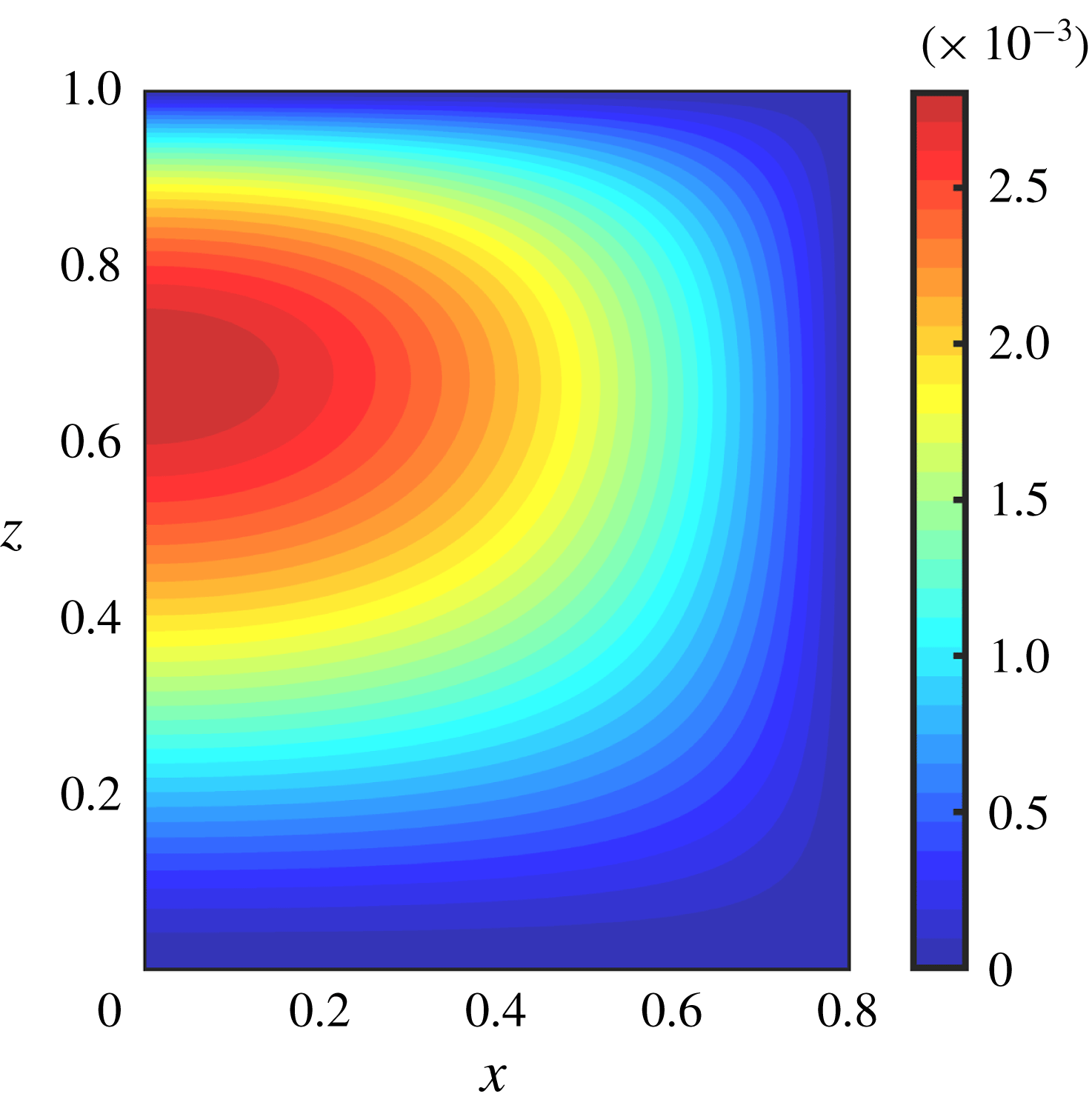In figure 11 we provide the first-order correction $h_{1}(x,z)$ to $h$ in order to identify any significant deviations from the leading-order form – the solution for $h_{1}$ is given by equations (2.29)–(2.30). Since the meniscus shape is a quantity that varies only in the intervals $0<x<\unicode[STIX]{x1D6FF}$ and $0<z<1$ , we can display $h_{1}(x,z)$ as a two-dimensional contour plot as seen in figure 11. The relatively small values achieved (less than $3\times 10^{-3}$ ) are a direct consequence of the relatively small values of $p_{1}$ observed in figure 9(b) – see solution (2.29) which tells us that $h_{1}$ depends linearly on $p_{1}$ . It is of note that the perturbations to $h$ are such that both $h_{0}$ and $h_{0}+\unicode[STIX]{x1D716}h_{1}$ represent circular arcs (up to an error of $O(\unicode[STIX]{x1D716}^{2})$ ). This is a consequence of the application of the Young–Laplace equation with constant (in each cross-section) pressure fields $p_{0}$ and $p_{0}+\unicode[STIX]{x1D716}p_{1}$ , respectively. Further inspection of figure 11 shows that the largest values of $h_{1}$ are in the vicinity of $x\sim 0$ , i.e. the meniscus centre, which might be expected as larger values of $h_{0}$ are achieved here. The overall maximum of $h_{1}$ is seen at a streamwise location of around $z=0.7$ , which corresponds to the maximum in $p_{1}$ found in figure 9(b). Physically, then, the correction $h_{1}$ will cause a local depression in the vicinity of $x\approx 0$ , $z\approx 0.7$ , something that could be of interest to experimentalists.

Figure 11.

Contour plot of the first-order correction $h_{1}(x,z)$ to the meniscus shape for $\unicode[STIX]{x1D6E4}=1$ , $H=0.5$ , $\unicode[STIX]{x1D6FF}=0.8$ .

5.2 Overall flow rates and the effects of inertia

The results of § 5.1 provided details of the flow-field, pressure distribution and meniscus shape up to two terms in the asymptotic expansion, hence yielding results correct to $O(\unicode[STIX]{x1D716}^{2})$ . To illustrate matters attention was focussed on one microchannel geometry having $H=0.5$ , $\unicode[STIX]{x1D6FF}=0.8$ and dimensionless surface tension $\unicode[STIX]{x1D6E4}=1$ . In this section we consider large ranges of $H$ , $\unicode[STIX]{x1D6FF}$ and $\unicode[STIX]{x1D6E4}$ and calculate their effect on the leading-order flow rate $Q_{0}$ and the scaled first-order correction $Q_{1}/(Re\,Q_{0})$ that introduces the effects of inertia. Recall that $Q=Q_{0}+\unicode[STIX]{x1D716}Q_{1}+\cdots \,$ , and expressions for $Q_{0}$ and $Q_{1}$ have been derived in (3.7) (equivalently (3.17)) and (3.8) (equivalently (3.52)), respectively, and calculated using quadratures once the leading-order and first-order quantities are determined. The Reynolds number $Re$ is included on the denominator of the quantity $Q_{1}/(Re\,Q_{0})$ because $Q_{1}$ is proportional to $Re$ – see (3.52). We can multiply with a given value of $Re$ to obtain the appropriate first-order flow rate as needed.

Before presenting results from the computations, we introduce two approximations to $Q_{0}$ and $Q_{1}$ denoted by $Q_{0}^{(approx)}$ and $Q_{1}^{(approx)}$ , respectively. Our motivation stems from the question of whether the flow rates constructed using 3-D effects (albeit for the slowly varying case) can be approximated well using computations of 2-D equations, i.e. Poisson solvers that avoid the need for computing transverse flow quantities as for example $u_{0}$ and $v_{0}$ . Mathematically this simplification avoids solving biharmonic equations for the modified streamfunction $\unicode[STIX]{x1D713}$ – see (3.19) and (3.22) – allied with singularity removal techniques for fourth-order problems as described in § C.3.

We begin with the approximation of $Q_{0}$ defined by

where $Q_{0}$ is given as a function of $p_{0}$ in (3.15). Instead of the exact form (3.17) for $Q_{0}$ , we approximate the integrand $\widetilde{Q}_{0}$ by its value in the middle of the $p_{0}$ -domain, i.e. at $p_{0}=1/2$ , leading to the (5.1). Note that this is exactly the two-dimensional approximation that assumes a constant pressure gradient, with the meniscus protrusion angle chosen to be that corresponding to the pressure midway between inlet and outlet pressures. Next, we define $Q_{1}^{(approx)}$ in the same way as $Q_{1}$ given by (3.8) or equivalently by (3.52), except that during the calculation process of $w_{C}$ via (3.38) we use the following approximations for the transverse velocities $u_{0}$ and $v_{0}$

Specifically, to calculate $w_{C}$ we substitute (5.2) for $u_{0}$ and $v_{0}$ into (3.38) and use the result to calculate $Q_{1}$ (now named $Q_{1}^{(approx)}$ ) as before. We anticipate this to be a good approximation as we expect $\unicode[STIX]{x1D713}$ to be numerically small globally (as indeed confirmed a posteriori from the full computations). The reason for this is that $\unicode[STIX]{x1D713}$ , as defined by (3.19) and satisfying the biharmonic equation (3.22) and relevant boundary conditions given in § 3.3, has $\unicode[STIX]{x1D713}=0$ imposed by boundary conditions on three sides of the domain.

Figure 12.

(a) The zeroth-order flow rate $Q_{0}$ and (b) the first-order flow-rate correction metric $Q_{1}/(ReQ_{0})$ plotted against $H$ for the indicated values of the liquid fraction $\unicode[STIX]{x1D6FF}$ and $\unicode[STIX]{x1D6FE}=1.2$ . In both cases dotted lines represent the corresponding approximate values $Q_{0}^{(approx)}$ and $Q_{1}^{(approx)}$ . Note that in both cases, but particularly in (a), the dotted lines are not easily visible due to very good agreement.

We begin by presenting results for $Q_{0}$ and $Q_{1}/(ReQ_{0})$ for a wide range of dimensionless microchannel heights $H$ describing narrow microchannels all the way to relatively high microchannels having $H=10$ . The results given in figure 12 were computed for $\unicode[STIX]{x1D6FF}=0.7,0.8,0.9$ , i.e. half-ridge lengths of 0.3, 0.2 and 0.1, respectively. The surface tension parameter is $\unicode[STIX]{x1D6E4}=1.2$ . The leading-order flow rate $Q_{0}$ is given in figure 12(a) and the correction $Q_{1}/(ReQ_{0})$ is included in figure 12(b). For each value of $\unicode[STIX]{x1D6FF}$ we also superimpose with dotted curves, the approximations $Q_{0}^{approx}$ and $Q_{1}^{approx}$ given above. The accuracy of such approximations is remarkable for the given range of $H$ , and this finding can have implications for practitioners. Firstly, the success of $Q_{0}^{(approx)}$ implies that for problems where inertial effects do not need to be considered, the technical details of the slowly varying approximation results do not need to be accounted for. A practitioner can simply take the midpoint of the inlet and outlet pressures, and compute the two-dimensional problem at this pressure. Secondly, the success of $Q_{1}^{(approx)}$ indicates that the most difficult and time-consuming part of the implementation of the methodology (solving the cross-flow problem) is often unnecessary for good accuracy. In fact, the implementation of this approximation will only require the solutions to a sequence of second-order problems. It also means that significant progress may be made in finding analytical solutions, as the fourth-order problem would have been the most significant barrier to this. We expect there to be a formal way to quantify the strength of these approximations using asymptotic analysis (with $H$ as a large parameter) as carried out in related problems, see Crowdy (Reference Crowdy2016), D. G. Crowdy (private communication, 2017), Kirk et al. (Reference Kirk, Hodes and Papageorgiou2017), Kirk (Reference Kirk2018).

The overall trends of the results for the leading-order flow rate $Q_{0}$ shown in figure 12(a) are as expected, namely smaller width ridges produce larger flow rates due to reduced flow resistance. The results also show that this is valid for all values of $H$ with the curve for $\unicode[STIX]{x1D6FF}=0.9$ yielding the highest values and $\unicode[STIX]{x1D6FF}=0.7$ the lowest ones. In addition, as expected $Q_{0}$ is monotonically increasing with $H$ for all values of $\unicode[STIX]{x1D6FF}$ computed.

Figure 13.

(a) The first-order velocity $w_{1}$ and (b) the leading-order velocity gradient $w_{0z}$ , plotted at $z=0,1/4,1/2,1$ (left to right). Other parameters are $\unicode[STIX]{x1D6FF}=0.8$ , $H=6$ .

Figure 12(b) also illustrates that $Q_{1}$ is more sensitive to $\unicode[STIX]{x1D6FF}$ as compared to $Q_{0}$ . The results also show that the behaviour of $Q_{1}$ with $H$ is non-monotonic with a negative minimum being attained at $H\approx 6$ . As explained in § 5.1, the correction $Q_{1}$ is negative for small and moderate values of $H$ mainly due to inertial terms and in particular $w_{0}w_{0z}$ being relatively large and positive compared to the other inertial terms and the correction $p_{1z}$ of the pressure gradient. Figure 12(b) also shows that at large values of $H$ it is possible to obtain positive values of $Q_{1}$ , implying flow-rate enhancement due to inertial effects. For example, $Q_{1}$ becomes positive for $H$ larger than approximately $7.7$ , $8.6$ or $9.5$ , for ridges characterized by $\unicode[STIX]{x1D6FF}=0.7$ , $0.8$ and $0.9$ , respectively. A physical explanation can be given both for the sign of $Q_{1}$ in this regime as well as the requirement of larger $H$ as $\unicode[STIX]{x1D6FF}$ increases and the ridge width decreases. For large $H$ the decrease in area towards the end of the microchannel becomes insignificant compared to the enhancement in slip length due to the flattening meniscus – see Game et al. (Reference Game, Hodes, Keaveny and Papageorgiou2017), Kirk et al. (Reference Kirk, Hodes and Papageorgiou2017), for example. This slip enhancement in turn enables the leading-order flow $w_{0}$ to decrease towards the centre of the microchannel to maintain a constant flow rate. This causes $w_{0z}$ to be negative in the centre of the microchannel away from boundaries, and hence the main inertial contribution $w_{0}w_{0z}$ is negative over a large region of the cross-section and acts as a favourable pressure gradient – see (3.34) and the relevant discussion in § 5.1. This then causes $w_{1}$ to become positive towards the centreline and once $w_{1}$ is positive over a sufficiently large part of the microchannel, the quantity $Q_{1}$ also becomes positive. For completeness, and to quantify the physical explanation given above, we provide numerical results of the streamwise velocity correction $w_{1}$ and the key quantity $w_{0z}$ , for a value of $\unicode[STIX]{x1D6FF}=0.8$ and two values of $H=6$ and $H=10$ – these results correspond to the middle curve in figure 12(b) with $H=6$ predicting a flow-rate decrease since $Q_{1}<0$ then, and $H=10$ corresponding to an increase in flow rate since $Q_{1}>0$ . Results for $H=6$ are depicted in figure 13 at the streamwise locations $z=0,1/4,1/2,1$ , with $w_{1}$ and $w_{0z}$ shown in figures 13(a) and 13(b), respectively. The results show that $w_{1}$ is mostly negative and $w_{0z}$ is mostly positive in the different cross-sections, explaining the negative value of $Q_{1}$ and hence the decrease in overall flow rate. The situation is the opposite when $H=10$ as shown in figure 14, with $w_{1}$ having large positive velocities in the majority of the microchannel driven by negative values of $w_{0z}$ .

Figure 14.

(a) The first-order velocity $w_{1}$ and (b) the leading-order velocity gradient $w_{0z}$ , plotted at $z=0,1/4,1/2,1$ (left to right). Other parameters are $\unicode[STIX]{x1D6FF}=0.8$ , $H=10$ .

Finally, in figure 15, we provide a more complete exploration of the parameter space, giving $Q_{1}/(ReQ_{0})$ as all three parameters $\unicode[STIX]{x1D6FF},H$ and $\unicode[STIX]{x1D6E4}$ vary in the ranges $0.5\leqslant \unicode[STIX]{x1D6FF}\leqslant 0.9$ , $0.5\leqslant H\leqslant 4$ and $1\leqslant \unicode[STIX]{x1D6E4}\leqslant 2$ . It is noteworthy that $Q_{1}$ becomes more negative for smaller $\unicode[STIX]{x1D6E4}$ , as can be seen by fixing $\unicode[STIX]{x1D6FF}$ in any of the figures and reducing the value of $\unicode[STIX]{x1D6E4}$ . This is quite intuitive since smaller $\unicode[STIX]{x1D6E4}$ leads to a larger inlet meniscus curvature and therefore enhanced three-dimensional effects. Similarly, increasing $\unicode[STIX]{x1D6FF}$ for a fixed $\unicode[STIX]{x1D6E4}$ also enhances the three-dimensional effects, which in turn causes $Q_{1}$ to become more negative.

Figure 15.

Contour plots of $Q_{1}/(ReQ_{0})$ against $\unicode[STIX]{x1D6E4}$ and $\unicode[STIX]{x1D6FF}$ for the indicated values of $H$ .