Implications
The e-Dairy model was designed to predict the biophysical and economic performance of grazing dairy systems, with some key variables allowed to behave stochastically, which enables the risk associated with different feed management strategies to be evaluated. The e-Dairy model can be used for different types of grazing dairy systems, that is, ryegrass- or lucerne-based systems with and without supplementation and for cows of different genetic merit.
This paper combines, within a whole-farm model, advances from previous models that predict milk yield, body lipid change and pasture intake at grazing, and presents a methodology to stochastically simulate cows of different genetic merit for several traits.
Introduction
System modelling involves the use of mathematical models to represent the key features of a complex system, in order to make quantitatively logical predictions about the system's performance (Woodward et al., Reference Woodward, Romera, Beskow and Lovatt2008). Thus, the modelling of dairy systems becomes a powerful tool to test the system's performance in a range of different conditions, including different market prices of milk and feeds, different policies and different values for genetic merit of cows.
Several whole-farm models simulate grazing dairy systems. Some of these models work at a herd level (Larcombe, Reference Larcombe1990; Freer et al., Reference Freer, Moore and Donnelly1997; Shalloo et al., Reference Shalloo, Dillon, Rath and Wallace2004; Schils et al., Reference Schils, De Haan, Hemmer, Van den Pol-Van Dasselaar, De Boer, Evers, Holshof, van Middelkoop and Zom2007; Vayssières et al., Reference Vayssières, Guerrin, Paillat and Lecomte2009), whereas other models work at an individual animal level (Beukes et al., Reference Beukes, Palliser, Macdonald, Lancaster, Levy, Thorrold and Wastney2008; Bryant et al., Reference Bryant, Ogle, Marshall, Glassey, Lancaster, Garcia and Holmes2010). These latter models account for genetic differences between cows, but they were designed to be used under specific conditions, that is, grass-based dairy systems and their environmental conditions under which the breeding values were estimated. The e-Dairy model, described in this study, differs from the aforementioned models in its ability to simulate the performance of individual cows, accounting for genetic differences between cows and genotype × environment interactions at an animal level (with genetic merit defined in such a way to not restrict the use of the model to a particular region), for both grass- and lucerne-based dairy systems.
Stochastic behaviour of the genetic merit of individual cows is seldom allowed in farm models. Gartner (Reference Gartner1981) simulated a dairy herd with cows accounting for differences in genetic merit for one trait, milk production. A distinctive feature of the model presented here is that it allows stochastic behaviour of the genetic merit of individual cows for several traits namely, yields of milk, fat and protein, live weight (LW) and body condition score (BCS), and also for the consequent energy requirements and dry matter (DM) intakes per cow, within a whole-farm model.
The whole-farm model, e-Dairy, is built upon the animal model e-Cow (Baudracco et al., Reference Baudracco, Lopez-Villalobos, Holmes, Comeron, Macdonald, Barry and Friggens2012), which simulates the performance of a single dairy cow at grazing. The prediction of energy partitioning within the cow, to either milk yield or body tissues, is a long-standing problem that has still not been solved (Friggens and Newbold, Reference Friggens and Newbold2007), particularly if the genetic merit of the cow and the genotype × environment interactions are to be considered. The present whole-farm model predicts body tissue mobilisation accounting not only for nutritional drives, but also for genetic drives, on the basis of the model of Friggens et al. (Reference Friggens, Ingvartsen and Emmans2004).
The e-Dairy model is designed to explore the effects of, and interactions between, cow genetic merit, supplementation and stocking rate, and their impact on biophysical and economic performance of grazing dairy systems, allowing stochasticity for milk and concentrate prices, genetic merit of cows and for the amount of pasture grown on farm.
The objectives of the present study are to describe and validate the e-Dairy whole-farm simulation model, and to illustrate the use of the model with stochastic simulations of grazing dairy systems, which explore the risk associated with two contrasting strategies of supplementation and stocking rate.
Material and methods
Model overview
The e-Dairy model is energy based, dynamic (daily simulation over a 365-day period) and is written in the Visual Basic programming language within Microsoft Excel®. Dairy farms with either ryegrass- or lucerne-based pastures, with or without summer or winter crops, and with any calving pattern can be simulated. An animal model, e-Cow (Baudracco et al., Reference Baudracco, Lopez-Villalobos, Holmes, Comeron, Macdonald, Barry and Friggens2012), was integrated into e-Dairy to simulate the performance of individual cows at grazing.
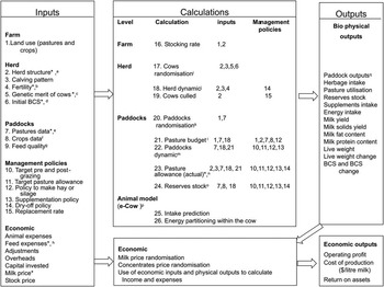
The main inputs of e-Dairy are farm area, use of land for either pasture and crops, type of pasture (ryegrass-based or lucerne-based), type of crops (winter or summer crop), monthly pasture growth rate (mean and s.d.; used to predict daily herbage mass (HM) for each paddock), annual crop yield (mean and s.d.), supplements offered, quality of feeds including NDF and metabolisable energy (ME), herd description including herd size, age structure, calving pattern, BCS at calving, probabilities of pregnancy, average genetic merit (potential yields of milk, fat and protein) and economic data for items of income, costs and assets. Stocking rate (cows/ha) is indirectly an input that is the result of the number of cows and the farm area, both set as inputs. The model allows to set management policies such as calving pattern, dry-off policy, target pre- and post-grazing HM, a policy to make hay or silage from pasture and supplementation. The main outputs are herbage and total DM intake, annual pasture utilisation, yields of milk, fat and protein, changes in BCS and LW, economic farm profit and return on assets. A global schematic representation of the model is shown in Figure 1.
Schematic representation of the e-Dairy model. *Can be set to behave stochastically. aHerd structure: number of cows per age category (year) and per lactation number. bFertility: probability of pregnancy at each service, calving system (seasonal or all-year-round) and number of services. cGenetic merit (potential yields of milk, fat and protein, parameters defining milk fat and milk protein content, target BCS parameters and live weight). dInitial BCS: mean and s.d. ePastures data: number and size of paddocks, pasture type, initial herbage mass and herbage growth rates (mean and s.d.). fCrops data: number and size of paddocks, type of crop (summer or winter), amount of DM produced/ha per year, the fate of the crop (grazing, silage or hay) and efficiency of harvesting or grazing. gFeed quality: NDF, metabolisable energy (ME) of herbage and supplements, and rate of herbage quality decrease/increase if not used by optimum date. hFeed expenses: concentrates price can be set to behave stochastically. iCows randomisation: to allocate a unique genetic merit to each cow, on the basis of average genetic merit and (co)variance matrix. jHerd dynamic: number of lactating and dry cows (daily). kPaddocks randomisation: to define initial herbage mass (HM) on each paddock. lPasture budget sub-routine that matches in advance the amount of pasture available with the amount of pasture required. mPaddocks dynamic: daily HM and actual growth rate, grazing dates and grazing time per paddock and actual post-grazing mass. nPasture allowance: actual kg DM offered per dry and lactating cow/day. oReserves stock: kg DM reserved as hay and silage. pe-Cow model: see schematic representation, inputs and equations in the e-Cow model (Baudracco et al., Reference Baudracco, Lopez-Villalobos, Holmes, Comeron, Macdonald, Barry and Friggens2012) explaining dry matter (DM) and energy intake and energy partitioning within the cow. qPaddocks outputs: daily actual pre- and post-grazing herbage mass, daily actual growth rates.

Cows
Each cow has unique values for the parameters defining its genetic merit, and the performance of each cow is individually simulated on a daily basis in e-Dairy, using the animal model e-Cow described in Baudracco et al. (Reference Baudracco, Lopez-Villalobos, Holmes, Comeron, Macdonald, Barry and Friggens2012). The e-Cow model is an energy-based model that predicts intakes of DM and energy, yields of milk, fat and protein and changes in BCS and LW. The main features of the e-Cow model are the combination of physical, metabolic and ingestive constraints in the prediction of herbage DM intake, the homoeostatic and homeorhetic control of body lipid change and its ability to predict performance of cows of different genetic merit.
There is now considerable evidence that genotype affects nutrient partitioning throughout differences in gene expression and enzyme profiles (Friggens et al., Reference Baudracco, Lopez-Villalobos, Holmes, Comeron, Macdonald, Barry and Friggens2012). The genetic merit of the cow, in the e-Cow model, is defined by her potential yields of milk, fat and protein (kg/cow for a 305-day lactation period), LW at calving and genetic targets for BCS at conception and at next calving. The genetic potentials and genetic targets are those achieved by the cow when no feeding restrictions are imposed; however, predictions are later adjusted by the nutritional status of the cow in our model (Baudracco et al., Reference Baudracco, Lopez-Villalobos, Holmes, Comeron, Macdonald, Barry and Friggens2012). This approach of homeorhetic-driven variables and homoeostatic corrections was already used by Martin and Sauvant (Reference Martin and Sauvant2010).
Potential milk yield is calculated in e-Dairy using a mathematical mammary gland model (Vetharaniam et al., Reference Vetharaniam, Davis, Upsdell, Kolver and Pleasants2003), which is based on the interaction of two pools of alveoli (i.e. groups of secretory cells): one active pool and one non-active pool. Further details are given in the description of the e-Cow model (Baudracco et al., Reference Baudracco, Lopez-Villalobos, Holmes, Comeron, Macdonald, Barry and Friggens2012). The default potential milk yields for mature cows (in a 305-day lactation period) are 11 247 and 8011 kg milk per cow, with 836 and 679 kg milk solids (MS; fat plus protein) per cow for North American (NA) and New Zealand (NZ) Holstein–Friesian (HF) strains, respectively. These are default values internally stored in the model. However, cows with different potential milk yield can be simulated by defining other potential yield of milk as inputs. When the input potential milk yield differs from the internally stored values cited above, an iterative procedure is used to find the value of parameters of the mammary gland model that produces a lactation curve with the new potential milk yield (kg milk for 305 days).
The potential yields of fat and protein (kg/cow in 305-day lactation) are the result of the sum of the product between daily potential milk yield and daily milk fat or milk protein concentration. Daily milk fat and milk protein concentrations are calculated using lactation curves produced with the Wilmink (Reference Wilmink1987) function:
 $${{y}_t}\,{\rm{ = }}\,a\,{\rm{ + }}\,b{{e}^{{\rm{ - 0}}{\rm{.05}}t}} \,{\rm{ + }}\,ct \eqno(1)$$
where yt represents the percentages of milk fat or milk protein at day t of lactation and e is the base of natural logarithm (2.718281828), whereas a, b and c are estimated parameters that define the scale and shape of the curve. The values for parameters a, b and c were obtained from a study by Roche et al. (Reference Roche, Berry and Kolver2006), for both NZ and NA HF cows.
The BCS and LW are modelled according to the genetically driven body lipid change model proposed by Friggens et al. (Reference Friggens, Ingvartsen and Emmans2004), with the main concepts of this model further expanded in a study by Friggens and Newbold (Reference Friggens and Newbold2007). This body lipid change model proposes that mobilisation and gain of body reserves are genetically driven to achieve two genetic targets of body fatness: one, at or around conception, and another at the next calving. In the e-Cow model, the genetically driven changes in LW and BCS (i.e. no nutritional constraints) are initially calculated and then adjusted on a daily basis according to the nutritional status of the cow. All equations and parameters used in the e-Cow model are described in detail by Baudracco et al. (Reference Baudracco, Lopez-Villalobos, Holmes, Comeron, Macdonald, Barry and Friggens2012). In the e-Cow model, the genetic merit of the cow is defined by the potential yields of milk, fat and protein, parameters a, b and c of the Wilmink function for milk fat and milk protein concentrations, LW and parameters defining target BCS at conception and at next calving.
Herd
Random generation of cows with correlated variables
Each cow is generated randomly through the following correlated traits: potential yield of milk, LW at calving and parameters of the Wilmink function defining milk fat and milk protein concentration curves (equation (1)). In order to simulate randomly a herd in which each cow has correlated values for all variables, the following matrix operation is performed:
 $$\bf H\,{\rm{ = }}\,m'\,{\rm{ + }}\,L\,{\rm{\times }}\,Z$$
where H is the matrix of the simulated herd, with each trait in a column and each cow in a row, m is the vector with the herd mean values for each trait (inputs), L is the lower triangular matrix obtained by Cholesky decomposition of the phenotypic (co)variance matrix (A) between the traits and Z is a matrix with random values derived from a normally distributed function with a mean of 0 and a s.d. of 1. A similar procedure has been used by Gartner (Reference Gartner1981).
Elements of the phenotypic (co)variance matrix A were estimated using phenotypic records from a trial comparing cows of NA and NZ HF strains (Macdonald et al., Reference Macdonald, Verkerk, Thorrold, Pryce, Penno, McNaughton, Burton, Lancaster, Williamson and Holmes2008b). The product between the vector Z that has random values (mean of 0 and a s.d. of 1) and the matrix L (containing information about traits variance and correlation between traits) creates the correlated variance for each cow on each trait. The m vector contains all the traits described as columns of the H matrix and represents the mean herd values for each trait. Thus, summing up m to the product L × Z, a unique value is allocated to each cow on each trait. The average values of the m vector are set as default for each strain (see e-Cow model, Baudracco et al., Reference Baudracco, Lopez-Villalobos, Holmes, Comeron, Macdonald, Barry and Friggens2012), but new values can be set as inputs. Each cow is further allocated an age (see the ‘age structure’ section) and a BCS at calving. The BCS at calving is defined as input (Figure 1), with a mean and s.d. for a normal distribution.
Age structure
The age structure of the herd is an input defined as the percentage of cows in each age category, that is, year. Then, each of the simulated cows of the H matrix is randomly given an age. Afterwards, potential milk yield and LW are age adjusted for each cow. The following multiplicative age adjustment factors are used to adjust potential milk yields: 0.75, 0.87, 0.95, 1.0, 0.97 and 0.92 for lactations 1, 2, 3, 4 to 7, 8 and 9, respectively (Lopez-Villalobos et al., Reference Lopez-Villalobos, Garrick, Holmes, Blair and Spelman2000). Multiplicative age adjustment factors for LW at calving are: 0.85, 0.92 and 0.96 for cows in first, second and third lactation, respectively (Fox et al., Reference Fox, Van Amburgh and Tylutki1999).
Paddocks
The number and size of paddocks with pasture and crops are inputs (Figure 1). In pasture paddocks, the net herbage accumulation rate depends on a general net herbage accumulation rate curve (input), but is affected by the particular HM of each paddock, which is altered by the events of grazing and its intensity (see the ‘HM, herbage accumulation and grazing dates’ section). This results in a unique growth rate on each paddock.
In paddocks with crops, the type of crop (summer or winter), the amount of DM produced/ha per year (mean and s.d.), the fate of the crop (grazing, silage or hay) and the grazing/harvesting efficiency need to be set as inputs. If the crop is grazed, the grazing efficiency is constant (input) for all crop paddocks and for all the grazing events, in contrast to what happens in paddocks with pasture, where grazing efficiency is predicted for every paddock and every grazing event (see the ‘simulation of grazing’ section). The response to fertiliser is not simulated, but could be indirectly accounted for by changing the input amount of DM produced/ha per year.
HM, herbage accumulation and grazing dates
Daily net herbage growth rates are required as an input (kg DM/day, average of each month; Figure 1). Herbage growth can behave either stochastically or deterministically – it is optional in the model. For deterministic simulations, the growth rates used are those set as inputs. For stochastic simulation, the input herbage growth rates are used as the mean of a normal distribution, and an s.d. is required as input to randomise the herbage growth rates. Thus, the effect of climate on herbage growth rate can be accounted for, by using s.d. obtained from experimental data sets.
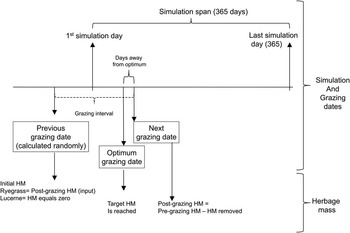
A ‘target pre-grazing HM’ (Figure 2), needs to be defined as input, expressed as kg DM for ryegrass-based pastures and as accumulated ‘growing degree days’ for lucerne pastures, which is an indicator of morphological development (Sanderson et al., Reference Sanderson, Karnezos and Matches1994). Daily minimum and maximum temperatures (inputs) are needed to calculate ‘growing degree days’. The date when each paddock reaches the ‘target pre-grazing HM’ is named ‘optimum grazing date’. However, the actual date of grazing, named ‘next grazing date’, may differ from the calculated ‘optimum grazing date’ (Figure 2) according to the use of paddocks. The calculated difference (days) between the ‘optimum grazing date’ and the ‘next grazing date’ is called ‘days away from optimum’, as shown in Figure 2. HM in each paddock will accumulate daily, from ‘previous grazing date’ until ‘next grazing date’, as shown in the timeline of Figure 2. The herbage growth rate set as input is affected by the grazing intensity, using the following equation (Garcia, Reference Garcia2000):
 $$ {\rm{Growth}}\,{\rm{rate}} = \left( {{\rm{GR}}\times \frac{{\rm{4}}}{{{\rm{H}}{{{\rm{M}}}_{{\rm{max}}}}}}} \right)\times {\rm{H}}{{{\rm{M}}}_{{\rm{(}}t{\rm{)}}}}\left( {{\rm{1 - }}\frac{{{\rm{H}}{{{\rm{M}}}_{{\rm{(}}t{\rm{)}}}}}}{{{\rm{H}}{{{\rm{M}}}_{{\rm{max}}}}}}} \right) $$
where GR is the input herbage growth rate (kg DM/day, input), HM(t ) is the HM of the paddock in the day of simulation, calculated as HM of the previous day (HM(t − 1)) plus GR, HMmax (input) is the HM at which net accumulation rate approaches zero because senescence rate approaches gross growth rate (Bircham and Hodgson, Reference Bircham and Hodgson1983).
Schematic representation of the simulation of grazing dates and herbage mass (HM) for each paddock within the e-Dairy model.

Simulation of grazing
Each paddock is individually grazed. The duration of each grazing event in each paddock ‘grazing time’, is calculated with the following equation:
 $$ {\rm{Grazing}}\,{\rm{time}}\,{\rm{(days)}}\, = \,\frac{{{\rm{Pre - grazing}}\,{\rm{HM}}\,\times \,{\rm{paddock}}\,{\rm{area}}}}{{{\rm{Total}}\,{\rm{allowance}}\,{\rm{per}}\,{\rm{day}}}} $$
where ‘total allowance per day’ is calculated as the summed allowance for all cows.
The post-grazing HM is calculated as the difference between ‘pre-grazing HM’ and ‘herbage removed at grazing’, the latter being calculated as the sum of daily herbage DM intake of all cows. Daily herbage DM intake is not assumed but predicted for each cow, as explained in the e-Cow model (Baudracco et al., Reference Baudracco, Lopez-Villalobos, Holmes, Comeron, Macdonald, Barry and Friggens2012). Pasture utilisation (%) is calculated as the kg DM/ha consumed at grazing, divided by the kg DM/ha annual pasture accumulation and multiplied by 100.
Feed quality
The quality of each feed is defined as inputs (Figure 1), through a monthly value for ME (MJ/kg DM) and NDF (%DM). The quality of the pasture, set as input, is affected when the paddock is used before or after the ‘optimum grazing date’. Pasture quality will decrease (ME decrease and NDF increase) if ‘next grazing date’ occurs after the ‘optimum grazing date’ and vice versa (Figure 2). The rate at which pasture quality increases or decreases is an input expressed as percentage of the values of ME and NDF.
Management policies
Grazing policy
Before the simulation starts, it is possible to define a policy related to the utilisation of pastures, through the following inputs: ‘target pre-grazing HM’, ‘target post-grazing HM’ and ‘target pasture allowance’.
Pasture budget
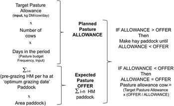
The date of grazing and the grazing time (per grazing event) in each paddock are calculated while the model runs; however, it is still possible to define a policy to use paddocks before the simulation starts. The automatic procedure implemented in the model to simulate paddocks dynamics is performed by a sub-routine named ‘pasture budget’ (Figure 3), which runs for a period defined with an input named ‘pasture budget frequency’. The pasture budget in e-Dairy consists of a calculation of future pasture offer (expected pasture offer) and future pasture demand (planned pasture allowance) for the whole farm. The ‘expected pasture offer’ is calculated as the sum of the product between pre-grazing HM in each paddock at the calculated ‘optimum grazing date’ and the area of each paddock (Figure 3). The ‘planned pasture allowance’ is calculated as the target pasture allowance per cow times the number of cows times the number of days in the period to be budgeted.
Schematic representation of the pasture budget performed in the e-Dairy model.

Hay and silage
A management sub-routine named ‘make hay or silage’ was implemented. There are two situations in which a paddock is allocated to hay or silage. The first can occur at the time of pasture budgeting. Thus, if the ‘expected pasture offer’ for the period is greater than the ‘planned pasture allowance’, whole paddocks will be conserved as hay or silage at its calculated ‘optimum grazing date’ (Figure 3).
The second situation is when a paddock, allocated to grazing at the pasture budgeting time, is not used by its ‘optimum grazing date’. In this case, the paddock remains available for grazing for a number of days (input). Once the ‘days away from optimum’ reaches the threshold value, all the pasture in the paddock is conserved as hay or silage.
Supplements
The following inputs define a supplementation policy: herd supplemented (lactating or dry), supplement type (concentrates, silage summer crop, silage winter crop, pasture silage, hay summer crop, hay winter crop and pasture hay), starting date, finishing date, kg DM/cow per day offered and efficiency of use (proportion of the offered supplement that is consumed).
Calving pattern
An input table is used to define the percentage of cows calving per week of the year. Then, a calving date is randomly given to each cow, on the basis of a flat probability function. A seasonal (any season), split calving or an all-year-round calving pattern can be defined.
Dry-off policy
In the e-Dairy model, lactation can be stopped at any stage by setting a dry-off policy (termination of lactation) on the basis of inputs of threshold values for either BCS or milk yield or the number of days until the cow calves again. When any of this threshold values is achieved, the lactation will finish. This policy is applied individually to each cow (Figure 1).
Fertility and replacement rate
In both all-year-round and seasonal calving systems, each cow is randomly allocated a mating date. For all-year-round systems, the mating date occurs after a voluntary waiting period defined with an input (days after calving, unique for each cow), whereas for seasonal systems mating will occur after a fixed number of days, also defined as input (days of simulation, common to all cows). For both calving systems, the probability of pregnancy at each service is defined as an input (Figure 1), and a flat probability function is used to randomly decide whether each cow gets pregnant or not, according to the probability of pregnancy set as an input at each service. The number of service is an input.
The number of cows to be replaced by heifers is defined as a percentage of the total number of cows as a single input (Figure 1).
Economics
Two different payment systems can be used, namely: price per litre of milk and multiple component price system (kilograms of fat × A + kilograms of protein × B − litres of milk × C), where A, B and C are the values per kilogram of fat and protein and litre of milk, respectively, as it is used in NZ (Marshall, Reference Marshall1989) and Ireland. The following groups of inputs are required: farm incomes, animal expenses, feed expenses, labour expenses, adjustments, overheads (includes depreciation) and assets. Items included in each section are based on DairyNZ (2009). This allows the calculation of two main outputs: operating profit [farm incomes − (animal expenses + feed expenses + labour expenses + adjustments + overheads)] and return on assets (economic farm profit ÷ assets × 100).
Simulation
Deterministic or stochastic simulations can be carried out with e-Dairy. The stochastic simulation allows multiple runs, which could represent either different farms in 1 year or different conditions for the same farm. A group of variables can be allowed to behave stochastically. Some variables are stochastically triggered at the beginning of the simulation (and stay constant), such as genetic merit of cows, initial BCS, calving dates, cows age, crops yield, milk price and supplement price and pasture growth rates, whereas other variables behave stochastically during the simulation, such as daily herbage allowance and probabilities of pregnancy. Probability distribution functions, and their respective parameters, need to be set as inputs for the stochastic simulation. The normal, flat and gamma functions are available in the model.
Outputs
The main system outputs are herbage DM intake per cow and per hectare, annual pasture utilisation, milk yield per cow and per hectare, annual changes in BCS and LW, economic farm profit and return on assets. However, daily values for each variable, for individual cows or individual paddocks are available after the simulation. Thus, outputs such as daily HM or post-grazing HM per paddock, daily milk yield, BCS and LW per cow are stored after the simulation.
Model validation
Two independent data sets resulting from stocking rate experiments, and not used in the development of the e-Dairy model, were used to validate the model. One data set was obtained from a farmlet trial comparing five levels of stocking rate (from 2.2 to 4.3 cows/ha) with HF cows, winter–spring calving, grazing on ryegrass-based pastures (offered 0.19 t DM supplement per cow/year) during 3 years in NZ (Macdonald et al., Reference Macdonald, Penno, Lancaster and Roche2008a). The second data set was obtained from a farmlet trial comparing three levels of stocking rate (from 1.6 to 2.6 cows/ha) with crossbred HF-Jersey cows, winter–spring calving, grazing on lucerne-based pastures (offered 1.8 t DM supplements per cow/year) during 2 years in Argentina (Baudracco et al., Reference Baudracco, Lopez-Villalobos, Romero, Scandolo, Maciel, Comeron, Holmes and Barry2011).
Measured inputs used to validate the model were stocking rate, monthly pasture growth rates, monthly amounts of supplements used per cow, monthly herbage allowances, monthly ME and NDF of pastures and supplements, weekly calving pattern, monthly pre- and post-grazing HM, farmlet averages for age structure, lactation length, BCS and LW at calving.
Annual outputs for actual and simulated farmlets were compared, with 21 points for validation (five farmlets during 3 years plus three farmlets during 2 years). Outputs compared were: yields of milk and MS (kg/cow per year), BCS and LW at day 365-day of simulation and annual pasture utilisation. The concordance correlation coefficient (CCC; Lin, Reference Lin1989) and the relative prediction error (RPE) (Fuentes-Pila et al., Reference Fuentes-Pila, Ibanez, De Miguel and Beede2003) were used to evaluate the extent of agreement between actual and predicted values. The Landis and Koch (Reference Landis and Koch1977) scale has been used here to describe the degree of concordance, with: 0.21 to 0.40 being ‘Fair’; 0.41 to 0.60 being ‘Moderate’; 0.61 to 0.80 being ‘Substantial’; and 0.81 to 1.00 being ‘Almost perfect’. The CCC reflects both precision, that is, the degree to which the predicted against actual values cluster about the regression line, and accuracy, that is, degree to which the regression line adheres to the 45° line through the origin.
The RPE is defined as the positive square root of the mean square prediction error (equation (5)), the latter expressed as a percentage of the mean of actual values (μA) (Fuentes-Pila et al., Reference Fuentes-Pila, Ibanez, De Miguel and Beede2003):
 $$ MSPE\, = \,\frac{{\rm{1}}}{n}\mathop{\sum}\limits_{i\, = \,{\rm{1}}}^n {{{{({{A}_i}{\rm{ - }}{{P}_i})}}^{\rm{2}}} } $$
where P represents the predicted values and A represents the actual observed values for either milk yield, MS yield, pasture utilisation, BCS or LW change. The RPE is used to decide whether the overall level of accuracy could be considered acceptable for practical use. Fuentes-Pila et al. (Reference Fuentes Pila, DeLorenzo, Beede, Staples and Holter1996) suggested that an RPE value <10% is an indication of satisfactory prediction, whereas an RPE between 10% and 20% indicates a relatively acceptable prediction, and an RPE >20% indicates poor prediction.
Results
Model validation
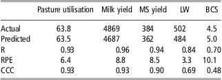
The accuracy of prediction of the e-Dairy model is shown in Table 1. Predicted data were compared with actual data from the NZ and the Argentine stocking rate trials.
Comparison of actual (Macdonald et al., Reference Macdonald, Penno, Lancaster and Roche2008a; Baudracco et al., Reference Baudracco, Lopez-Villalobos, Romero, Scandolo, Maciel, Comeron, Holmes and Barry2011) and predicted (e-Dairy) data for annual pasture utilisation (%), annual yields of milk (kg/cow), annual yield of MS (kg/cow), LW (kg/cow) and BCS (scale 1 to 10) at day 365 of simulation
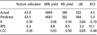
MS = milk solids; LW = live weight; BCS = body condition score; R = Pearson correlation coefficient; RPE = relative prediction error; CCC = concordance correlation coefficient.
The validation data set comprises data from 21 farm lets.
In validation analysis, the e-Dairy model showed satisfactory accuracy of prediction, with RPE <10% and with CCC over 0.80 for annual pasture utilisation, yields of milk and MS, and CCC of 0.69 and 0.48 for LW and BCS score at the end of the 365-day period, respectively (Table 1).
Average predicted values were close to average actual values. The model underpredicted annual pasture utilisation (−0.3%), milk yield (−182 kg/cow per year), MS yield (−22 kg/cow per year), LW (−18 kg per cow) and overpredicted BCS (+0.5, scale 1 to 10) at the end of the 365-day period (Table 1).
Model simulations
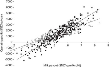
As an example of the practical application of the e-Dairy model, two owner-operated NZ dairy farms were stochastically simulated. One farm, named ‘low input’, was set to be similar to the average NZ dairy farm (LIC, 2010; DairyNZ, 2010), with 360 cows on 128 effective hectares (2.8 cows/ha) and 0.15 t DM/cow per year of imported supplement. The second farm, named ‘high input’, had 448 cows on 128 effective hectares (3.5 cows/ha) and 1.45 t DM/cow per year of imported supplement. In both cases, NZ HF cows (average LW of 477 kg) were simulated and calving started on 20 July. In both farms, pasture DM produced on farm was set to behave stochastically, using a normal distribution with a mean of 13.5 (s.d. = 1.25) t DM/ha per year. Milk payout per kg MS and concentrate price were also set to behave stochastically, using a normal distribution with a mean of $NZ 5.3/kg MS (s.d. = 1.13) and $NZ 0.45/kg DM (s.d. = 0.112), respectively, whereas all other inputs were held constant. Variables set to behave stochastically were assumed to be independent to each other.
Each farm was stochastically simulated 250 times. Average MS yields per cow were 334 ± 43 and 439 ± 36 kg MS/cow for low and higher input farms, respectively. The average MS yields per hectare per year were 941 ± 120 kg MS/ha per year in the low input farm and 1534 ± 127 kg MS/ha per year in the high input farm. However, operating profits were similar, with 1681 ± 1004 and 1703 ± 1272 $NZ/ha per year for the low and high input farms, respectively.
Discussion
The e-Dairy model was designed to predict the biophysical and economic performance of milk production systems and to explore the interactions between genetic merit, supplementation, stocking rate and market prices for systems using either ryegrass- or lucerne-based pastures. The e-Dairy model was designed to evaluate dairy farm systems over the whole year rather than short-term changes, that is, within 1 year.
Whole-farm models for grazing dairy systems that account for genetic differences between cows (Farmax Dairy Pro and WFM) are restricted to specific conditions, such as the type of pasture and the type of cow used in a particular region of the world. The e-Dairy model is relatively flexible in these respects, as it includes equations to predict herbage DM intake from both ryegrass- and lucerne-based pastures. In addition, the genetic merit of the cow is defined by several parameters including potential milk, fat and protein yield, LW and other parameters (Baudracco et al., Reference Baudracco, Lopez-Villalobos, Holmes, Comeron, Macdonald, Barry and Friggens2012), which do not restrict the use of the model to a particular region, opposite to the use of breeding values. Breeding values represent objective parameters to estimate potential production of dairy cows; however, the information provided by breeding values only reflects the potential production under the environmental conditions where the breeding values were estimated.
Most of the models predicting nutrient partitioning do not accommodate genotype. One reason for this is related to the difficulty of obtaining operational descriptions of genotype with respect to nutrient partitioning (Friggens et al., Reference Baudracco, Lopez-Villalobos, Holmes, Comeron, Macdonald, Barry and Friggens2012). The approach used to define potential yields in the e-Dairy model is based on productions achieved by cows under experimental conditions, where feed quantity and quality were not limiting (no major nutritional limitations). However, this does not mean that the actual genetic merit of the cow is known, but it is a pragmatic approach to define potential genetic merit.
Model validation
In validation tests, using the measured annual outputs of experimental farmlets, the model predicted with a high degree of accuracy (CCC > 0.80 and RPE < 10%) for annual pasture utilisation, and per farmlet annual yields of milk and MS. The accuracy of prediction was moderate for LW and BCS, when considering the CCC (Table 1). These levels of accuracy of prediction for DM intake and milk yield are similar or higher than those reported for other models for grazing dairy systems, such as Farmax Dairy Pro (Bryant et al., Reference Bryant, Ogle, Marshall, Glassey, Lancaster, Garcia and Holmes2010), GrazeIn (Delagarde et al., Reference Delagarde, Valk, Mayne, Rook, Gonzalez-Rodrıguez, Baratte, Faverdin and Peyraud2011) and the WFM (Beukes et al., Reference Beukes, Palliser, Macdonald, Lancaster, Levy, Thorrold and Wastney2008). However, it is important to notice that the validation of the model was conducted for annual outputs, and the accuracy of the model for short-term predictions (weekly or monthly basis) remains to be tested.
Model simulations
The stochastic simulation carried out for two contrasting dairy farms (Figure 4) shows the ability of the model to predict biophysical and economic performance of dairy systems, accounting in this case, for the risk associated with changes in pasture grown, milk price and concentrate prices, with all other inputs were held constant. Although the average profit per hectare was similar between the simulated systems, high input farms showed higher variation in terms of economic profit, showing both the greatest and the lowest values of profit per hectare (Figure 4), which is associated with higher risk.
Stochastic simulations carried out with e-Dairy for biophysical and economic performance of ryegrass-based dairy farms owner operated in New Zealand. (○) Low input systems with 2.8 cows/ha and 0.15 t DM/cow per year of imported supplement and (▪) high input systems with 3.5 cows/ha and 1.5 t DM/cow per year of imported supplement. Pasture grown, milk payout and concentrate price were allowed to behave stochastically using a normal distribution, whereas all other variables were held constant.

Figure 4 shows that at milk prices lower than $NZ5.5/kg MS, the lower input system was more profitable than the higher input system, whereas at prices higher than $NZ5.5/kg MS the opposite occurred. These examples show the potential of the model to explore the effects feeding level (stocking rate and supplementation) on economic outputs, when facing uncertainty in terms of pasture grown, milk price and supplement price.
The e-Dairy model can simulate different farms of a region by generating, stochastically, herds with differing genetic merit across farms. This, in turn, when combined with stochastic behaviour of pasture grown, can represent two of the most important features for a group of pasture-based dairy farms.
Model limitations
The e-Dairy model does not link BCS to fertility, and does not include health issues. However, the simulation of the effects of BCS on fertility could be implemented in future work by using the calculated daily BCS and BCS change of each cow to predict probabilities of pregnancy, with fertility as a function of BCS and BCS change. Similarly, the effect of health problems on the performance of cows could be simulated with a probabilistic approach supported by experimental data for the main health problems of dairy herds, such as mastitis and lameness.
At the current stage of development, the e-Dairy model is based only on energy, because protein supply does not usually limit milk production in grazing dairy systems (Holmes and Roche, Reference Holmes and Roche2007). However, there may be excess protein in leafy spring and especially autumn pastures with an associated energy cost in excreting the excess protein, or lack of adequate protein in diets with a high proportion of maize silage. In these cases, the inclusion of a protein balance would improve predictions.
The model evaluates the risk associated with changes in prices of milk and concentrates and pasture grown; however, as the model simulates only a 365-day period, risk aspects related to the management of the stocks throughout the years cannot be considered.
Conclusions
This model simulates pasture-based dairy farms. Three important features of the e-Dairy model are its ability to simulate, randomly, individual cows with internally correlated variables, its ability to account for genetic differences between cows and its ability to account for genotype × environment interactions. The model was proven to simulate annual performance of dairy cows with acceptable levels of accuracy for both ryegrass- and lucerne-based dairy systems.
The e-Dairy model can be used to explore the effects and interactions of feeding level and genetic merit of cows, for grazing dairy systems with differing calving patterns, evaluating the trade-offs between profit and the associated risk.
Acknowledgement
The authors thank Marcelo Zamateo for his support in the development of this model.
Supplementary materials
For supplementary material referred to in this article, please visit http://dx.doi.org/doi:10.1017/S1751731112002376