1 Introduction
Annuities provide a means by which risk-averse households facing an uncertain lifespan can insure themselves against the risk of outliving their wealth. Yet, only 7.4% of a large sample of elderly households in the United States had voluntarily purchased an annuity between 1993 and 2000 (Dushi and Webb, Reference Dushi, Anthony and Pierre-Andre2006). These purchases represent only a small proportion of household wealth held in annuitized form, though, because considerable household wealth is automatically annuitized through Social Security and defined benefit (DB) pensions offered by employers. The average married couple turning 65 between 1994 and 2000 had $248,778 in Social Security wealth and $154,810 in defined benefit pension wealth (Dushi and Webb, Reference Dushi and Anthony2004).
Annuity providers – be they insurance companies, private and public sector employers offering DB pension plans, or taxpayers through Social Security and the Pension Benefit Guaranty Corporation – face two kinds of mortality risk: idiosyncratic risk, since any particular annuitant may live longer than expected, and aggregate mortality risk, since annuitants may on average live longer than expected.Footnote 1 Idiosyncratic risk can be eliminated by increasing the size of the annuitant pool, but aggregate mortality risk cannot.
Friedberg and Webb (Reference Friedberg and Anthony2007) evaluate the consequences of aggregate mortality risk faced by voluntary annuity providers. To calculate the magnitude of this risk, they use the Lee and Carter (Reference Lee and Lawrence1992) mortality model, which – according to Deaton and Paxson (Reference Deaton, Christina and David2004) – has become the ‘leading statistical model of mortality in the demographic literature’.Footnote 2 Friedberg and Webb conclude that an insurance company using the Lee–Carter model to price annuities would face a 5% chance that the present value of its payments would be 3–4% greater than expected, and a 1% chance that they would be 5–6% greater.
Only a small part of aggregate mortality risk is held by insurance companies selling voluntary annuities, however. The vast majority is held by shareholders of companies providing DB plans to employees, by insurance companies providing deferred annuities to pension plans, and by taxpayers.Footnote 3 We extend the above research to consider the aggregate mortality risk faced by providers of DB pension plans. DB pension coverage has declined substantially in recent years in both the United States and the United Kingdom, and aggregate mortality risk is one of the factors that has explicitly been blamed in the UK (ACA, 2005: 13–14).Footnote 4 New UK reporting regulations just enacted in January 2007 are expected by some to reveal that plans have considerably underestimated expected participant longevity, which may in turn raise awareness of aggregate mortality risk and perhaps accelerate the rate of plan closures.Footnote 5
We consider two aspects of aggregate mortality risk: the possibility that plan providers use mortality forecasts that are biased upward, compared to Lee–Carter or to Social Security Administration (SSA) forecasts, and the possibility that future mortality rates are lower than those predicted by these up-to-date, putatively unbiased forecasts.Footnote 6 We first consider the likely consequences of any bias in plan providers' mortality assumptions, a concern that has recently been noted by regulators in the UK.Footnote 7 Our enquiries and previous research indicate that, by common practice, plan providers base the estimated pension liabilities reported in their financial statements on GAM83, a period mortality table reflecting 1983 mortality.Footnote 8 Very recently, there has been a shift towards RP2000, a period table reflecting mortality in the year 2000. Though GAM83 incorporates a 10% conservative margin, mortality rates have declined since both tables were compiled, and most forecasts project further declines. Our investigations further indicate that only a minority of plans adjust the period mortality table (e.g., GAM83 or RP2000) to reflect subsequent declines in mortality rates, and that any adjustments are typically made only to a current date and not over the expected lifetimes of plan participants.
We calculate the effect of this apparent forecasting bias on plan providers' pension liabilities. We find that, for older workers, the 10% conservative margin in GAM83 projected to a current date approximately offsets the effect of the mortality declines currently projected by the SSA over the remainder of the workers' lifetimes, and for retirees it more than compensates. For such workers in a plan that was experiencing typical group annuitant mortality in 1983, therefore, projecting GAM83 to a current date is expected to suffice. However, liabilities would be substantially understated for plans with younger workers (unless those plans projected mortality improvements over the whole of their workers' lifetimes) and for any plan that does not project. For males, the understatement could reach as much as 16.2%, depending on the ages of participants, if mortality rates decline at the rates predicted by the SSA in their intermediate assumptions. If mortality declines at the somewhat higher rates predicted by the Lee–Carter model, then the understatement could reach 22.4%. For females, the understatements could reach 6.1% and 11.4%, respectively.
We then consider the magnitude of risk inherent in an unbiased forecast of mortality improvements. We conclude that the rate of mortality decline is subject to considerable volatility over the time horizons that concern pension providers. We evaluate the effects of this volatility by running Monte-Carlo simulations of the evolution of aggregate mortality according to the Lee–Carter model and then calculating the impact of these mortality shocks on the projected benefit obligation of continuing pension plans.Footnote 9 In doing so, we assume that the Lee–Carter model provides an unbiased forecast and, importantly, that the confidence intervals capture the degree of uncertainty attached to that forecast. Our results are driven by that uncertainty and not by the predicted rate of decline. We calculate that there is, in any year, a 5% chance that an aggregate mortality shock raises a provider's projected benefit obligation for male participants by at least 1.04%, and a 1% chance that a shock raises it by at least 1.50%. The respective results for female participants are 0.85 and 1.19%. We also compute the impact on the present value of obligations faced by frozen plans. For a hypothetical plan, there is a 5% (1%) probability that reductions in aggregate mortality over the life of the plan raise the present value of total future payments for male workers by at least 3.3% (4.0%) above what is expected. Lastly, we evaluate the aggregate mortality risk faced by S&P 500 companies, using data supplied by Credit Suisse First Boston (2006). We conclude that, while the aggregate risk is not large relative to overall profits and stock market capitalization, it is quite substantial for a minority of companies.
The riskiness of the liability is sensitive to the interest rate used to discount the payments, being substantially greater at lower rates. One important implication is that inflation-protected pensions expose a provider to substantially greater aggregate mortality risk than nominal pensions, whose present value is calculated using a higher nominal rate of interest. Also, the percentage increase in time-discounted liabilities from a given mortality shock is somewhat greater for pension providers than for insurance companies selling immediate annuities, as calculated in Friedberg and Webb (Reference Friedberg and Anthony2007) using a similar approach. In contrast to an immediate annuity, which, as its name suggests, comes into payment immediately, a pension is a deferred annuity, exposing the provider to only the high-risk long time-horizon obligations.
Our results suggest a role for capital markets to reallocate aggregate mortality risk to those most willing to bear it. Longevity bonds have been proposed as a mechanism to transfer aggregate mortality risk efficiently from annuity providers to financial markets.Footnote 10 The payments on such bonds would be based upon the survival rate of a reference population, for example American males aged 65 in 2006. Purchasing the bonds would insure an annuity provider against aggregate mortality risk to the extent that the provider's mortality experience mirrored that of the reference population.
The remainder of the paper is organized as follows. In Section 2, we discuss the literature on trends in life expectancy and the Lee–Carter model. In Section 3, we explain how plan providers typically forecast mortality rates. We estimate the impact of forecasting bias on pension obligations and calculate the impact of putatively unbiased estimates of aggregate mortality risk. Section 4 concludes.
2 Modeling improvements in human longevity
In this section, we introduce the Lee–Carter mortality model. We discuss its usefulness in making aggregate mortality forecasts over the long time horizons faced by pension providers and for quantifying the risks associated with those forecasts, and we discuss competing models.
There is considerable disagreement about the scope for improvements in human longevity over long time horizons (Siegel, Reference Siegel2005). This disagreement sometimes pits ‘pessimistic’ biologists, who argue that we may be approaching biological limits to longevity, versus ‘optimistic’ mathematical demographers. To illustrate, Olshansky et al. (Reference Olshansky, Bruce and Christine1990) argue from the biodemographer's perspective that the average of male and female life expectancy is unlikely to rise beyond 85 years in any country. In contrast, Oeppen and Vaupel (Reference Oeppen and James2002) analyze ‘best practice’ life expectancy, selecting the maximum across countries in each period between 1840 and 2000. Since female life expectancy has risen at a fairly constant 2.5 years per decade, they conclude that we have not yet been affected by any biological limits to longevity, and that life expectancy at birth will attain 100 years in some countries around the year 2060. Similarly, Tuljapurkar and Boe (Reference Tuljapurkar and Carl1998) argue that neither theory nor evidence point to an irreducible component of mortality, while Sanderson and Scherbov (Reference Sanderson and Sergei2004) point out that life expectancy in the leading country is already nearing 85 years, that the rate of increase in this ‘best practice’ life expectancy is very nearly linear, and that there is little statistical evidence of a biological barrier to longevity. Some biologists disagree with the pessimistic view too, and Steven Austad, another famous researcher in the field, has wagered $500 million with Jay Olshansky that someone recently born will live to 150 by 2150.
The mathematical demography approach is extremely useful for making precise aggregate mortality forecasts. We employ the Lee and Carter (Reference Lee and Lawrence1992) model, which is, as we described earlier, the most widely used model of population mortality improvements. The Lee–Carter model has been adopted by the US Census Bureau, among others, and was viewed favorably by the Social Security Administration's 1999 technical advisory panel.Footnote 11 Lee–Carter found that, within age groups, their fitted model explains well over 90% of the variance in mortality rates. An attractive feature of the model is that it yields estimates of not only the expected rate of mortality decline, but also the probability distribution of outcomes.
In the Lee–Carter model, mortality risk m at age x in year t is

The parameters a and b vary with age. Lee–Carter estimate that a random walk with drift fits the time path of k, as follows

where flu is the impact of the 1918 epidemic.Footnote 12 We calculate that a one standard-deviation shock to k translates into a roughly two-month change in age-65 life expectancy. This specification implies no mean reversion in mortality trends, so a shock to current mortality yields an equal percentage change in all subsequent periods' expected mortality. The linear k trend translates into a constant percentage decline in mortality at any given age, and therefore a decreasing rate of increase in life expectancy. This is less extreme than either the optimistic view that life expectancy will continue to increase at about the rate experienced in the past, or the pessimistic view that life expectancy is inherently limited to around the age of 85.
The Lee–Carter model predicts that mortality among people over 65 will decline at a rate of 1.13% a year. This is considerably higher than the intermediate forecast by the SSA of 0.47% a year, increasing to 0.67% a year by 2029, and it is even high relative to the high forecast of 0.70% a year rising to 1.17% a year by 2029. Both forecasts lie within the Lee–Carter model's 95% confidence interval, in contrast to the low forecast of the SSA.
There are three reasons why forecasts made with the Lee–Carter model might transpire to be incorrect. The first is that realizations of the e t and e x,t error terms are zero in expectation but are of course likely to take other values. The e x,t term has little impact on the value of annuities because it affects only one period's mortality and is therefore disregarded in our simulations. In contrast, realizations of the e t term affect mortality not only this year, but also in all future years. The second possible source of error arises because, as with any statistical model, the parameters a x, b x, and k are estimated and not known with certainty. Lee and Carter (Reference Lee and Lawrence1992) show in an appendix that these sources of error are relatively unimportant. We nonetheless incorporate this source of uncertainty in our simulations. The third source of error is that the model may be mis-specified, or that it fails to capture the probability of an event so rare that it does not appear in the historical data, or simply that the future turns out to be unlike the past (Turner, Reference Turner2006).
The 95% confidence interval of Lee–Carter forecasts for the next 50–60 years encompasses much of the disagreement as to whether, when, and by how much, a deceleration in longevity gains will occur. It covers both the 2.5-years-per-decade linear increase in life expectancy at birth forecast by Oeppen and Vaupel (Reference Oeppen and James2002) and also a gradual deceleration in the rate of increase, as the point estimate in 2060 is 1.65 years' increase in life expectancy at birth per decade. It predicts with 20% probability that population life expectancy at birth in 2060 will be more than the 100 years predicted by Oeppen and Vaupel. On the other hand, the model attaches perhaps too low a probability – less than 0.1% – to the other extreme view, that life expectancy at birth in 2060 will be as low as the 85 years predicted by Olshansky et al. (Reference Olshansky, Bruce and Christine1990). However, this ‘upside’ risk is of much less concern to pension plan providers. Lee and Miller (Reference Lee and Timothy2001) critique the Lee–Cater model and conclude that, ‘for forecasts of life expectancy at birth up to 50 years into the future, the probability bounds are too broad rather than too narrow’, suggesting that use of the original model will, if anything, somewhat overstate aggregate mortality risk.
A variety of authors have proposed related specifications or further enhancements to Lee–Carter's work.Footnote 13 These potential improvements in the model are not generally important for our application, as is discussed at length in Friedberg and Webb (Reference Friedberg and Anthony2007). Nevertheless, we will mention a few points that may be relevant. There may be a small risk that medical breakthroughs will dramatically boost longevity, or conversely that an epidemic of obesity and diabetes may reduce it.Footnote 14 For example, Olshansky et al. (Reference Olshansky, Bruce and Christine1990) calculate that eliminating cancer, all circulatory diseases, and diabetes would raise male and female life expectancy at age 50 by 15.30 and 15.02 years respectively, equivalent to a 75% reduction in mortality rates. This small risk increases with the time horizon and may be understated by the Lee–Carter model. Based on Lee–Carter, we calculate that such a reduction has even less than a 0.01% probability of occurring over a 30-year period. Because we have no means of quantifying the extent to which the Lee–Carter understates the risk of dramatic mortality improvements, we restrict ourselves to sensitivity analyses later on.
3 Quantifying the aggregate mortality risk faced by defined benefit plans
In this section, we describe how pension funds treat mortality risk in practice, and we evaluate these assumptions taking, alternately, the Lee–Carter model and Social Security Administration forecasts as unbiased benchmarks. We consider the effect of the apparent forecasting bias on plan providers' pension liabilities, and then the effect of aggregate mortality risk on putatively unbiased estimates of these obligations. Finally, we consider mortality risk in relation to actual plan providers' profits and stock market capitalizations.
3.1 Evaluation of plan providers' mortality assumptions
Pension providers must report their accumulated and projected benefit obligations on Form 10-K. The 10-K statements about mortality assumptions are usually uninformative. For example, one large company reports that, ‘mortality rates are based on actual and projected plan experience’.Footnote 15 Watson Wyatt collects annually the only survey data of companies' actuarial assumptions of which we are aware.Footnote 16Watson Wyatt (Reference Watson2006) reports that 53% of surveyed plan providers use the GAM83 mortality table. Of those, only 1% use age setbacks for males and 6% do so for females, while only 9% of plans use mortality projections for both males and females.Footnote 17
Our own discussions with members of the actuarial profession yield similar conclusions about typical actuarial assumptions. We are informed, further, that only in the very largest plans do mortality tables and projections incorporate the plan's actual mortality experience. We understand that in the minority of cases where mortality is projected forward from GAM83 or RP2000, the projection is most often made only to a current date, with no continued improvements projected in the future. Whether they are projecting to the current date or beyond, the plan provider will typically use Projection Scale AA. Friedberg and Webb (Reference Friedberg and Anthony2007) show, however, that the Lee–Carter model predicts faster mortality declines than Scale AA, so even the small minority of plans that fully project using Scale AA may overestimate mortality.
The GAM83 mortality table includes a 10% reduction in mortality probabilities that provides some margin to absorb longevity increases. Our analysis of SSA period mortality tables indicates that male mortality among the over 60s had declined to 10% below 1983 levels by 1991, and to 21.4% below by 2005. In contrast, female mortality in 2005 was only 1.9% below the 1983 level. We calculate that if a pension plan had average group annuitant mortality in 1983, equal numbers of men and women participants, and population level mortality declines from then onwards, GAM83 approximates to current mortality.
Our discussions with actuaries indicate that in the past couple of years there has been a move towards using the RP2000 table. RP2000 is based on mortality experience from 1990 to 1994, projected to 2000, but lacks the 10% cushion of GAM83. Watson Wyatt (Reference Watson2005) show that, although RP2000 predicts lower male mortality than GAM83, the reverse is true for women, reflecting the above differences between male and female mortality declines since 1983.
In contrast to pension plans, which, as we have seen, often use outdated mortality tables, actuarial guidelines require insurance companies in the annuity business to develop ‘prudent best estimates’ of mortality, while regulators require them to retain financial reserves against adverse mortality experience and investment returns. For a pension plan, the firm's equity is a ‘financial reserve’, yet pension plans are, as we discuss later, exposed to greater aggregate mortality risk by reason of the longer duration of their liabilities.
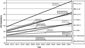
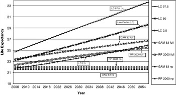
Figures 1(a) and (b) shows how the various mortality tables and projections translate into life expectancy for people reaching age 60 between 2006 and 2056. For convenience, the graphs show unisex mortality rates weighted by the projected proportions of men and women in the population by age. The horizontal lines show unisex life expectancy as predicted by the SSA 1983 and 2000 period tables (Figure 1(a)), and GAM83 (with the 10% margin) and RP2000 (Figure 1(b)). The upward-sloping lines in Figure 1(a) are for SSA's 2005 low, intermediate, and high mortality forecasts, and for the 2.5, 50, and 97.5 percentiles of the Lee–Carter forecasts from a jumping-off point of 2005 period mortality.Footnote 18 Those in Figure 1(b) are for GAM83 and RP2000, projected using Scale AA.
Life Expectancy at age 60 Under Lee-Carter and SSA Mortality Assumptions

Life Expectancy at age 60 Under Lee-Carter and Commonly Used Life Tables

Among the flat projections, the SSA 1983 and 2000 period life tables show shorter life expectancy than the corresponding pension annuitant life tables, reflecting the fact that the group annuitants represented in the GAM83 and RP2000 forecasts have relatively low mortality. The difference between GAM83 and the SSA 1983 period table (1.67 years) is greater than the difference between RP2000 and the SSA 2000 period table (0.57 years) because of the 10% conservative margin built into GAM83, but not RP2000.
The SSA intermediate forecast predicts a sex-weighted life expectancy at age 60 in 2006 of 22.60 years. The weighted-average low and high forecasts are 21.80 and 23.55 years, respectively. The SSA high projection is close to the central forecast obtained from the Lee–Carter model, reflecting the relative pessimism of the SSA forecasts. The SSA low projection lies increasingly below the 2.5 percentile of the Lee–Carter projection. Notably, though, both of them show continuing gains in life expectancy to levels considerably above both 1983 and 2000 period life expectancy. The life expectancies predicted by the SSA cohort tables and by Lee–Carter eventually far surpass GAM83 and RP2000, even though the predictions of the latter somewhat exceeded the 1983 and 2000 SSA life tables. So, a pension plan provider using GAM83 or RP2000 without any projection would underestimate longevity by increasing amounts, even if plan participants had population mortality rather than the somewhat lower mortality suggested by a comparison of RP2000 with the 2000 period mortality table. Another factor to consider is the socio-economic status of plan participants, which might lead to differences in not only current mortality but also the rate of decline. Scahlick et al. (Reference Schalick, Miller, Hadden, Elsie, Vicente and Gregory2000) found evidence of widening socio-economic mortality differences using older US data from 1967 to 1986, but it is difficult to infer whether mortality differentials have continued to expand.Footnote 19
Lastly, Figure 1 indicates how the uncertainty surrounding mortality forecasts – the source of aggregate mortality risk – rises with forecasting horizons. Though not interpretable as a confidence interval, the difference between the SSA high and low projections of life expectancy rises from 1.75 years in 2006 to 6.06 years by 2056. The 95% confidence interval in the Lee–Carter model, which was quite narrow in 2006 at only 2.72 years, rises to 7.06 years by 2056.
3.2 The impact of forecasting bias on pension liabilities
Our discussion above suggests that many pension providers are using outdated mortality forecasts. In this subsection, we consider the impact of this apparent forecasting bias compared to Lee–Carter and SSA forecasts, and in the next we evaluate the magnitude of aggregate mortality risk in those putatively unbiased forecasts. We will determine the impact of mortality risk on two measures of DB pension liabilities – the projected benefit obligation of continuing plans and the accumulated benefit obligation of frozen plans. The former accounts for projected salary increases of current workers until retirement, while the latter is based on current salary, as described in the Appendix. Projected benefit obligation is based on employees' service to date, and ignores the impact of mortality risk on the provision of benefits in relation to future service – so we underestimate the consequences for employers if employees do not end up taking lower cash wages to bear mortality-related increases in the cost of providing future benefits.Footnote 20
As previously discussed, plan providers could (and do) make a wide variety of mortality assumptions. They could use GAM83 or RP2000 with no projection, projection to 2006, or full projection into the relevant future (and until very recently most seem to have used GAM83 with no projection). We refer to these generically in our tables as ‘providers’ mortality assumptions.' A variety of assumptions about projections of future mortality are also possible. One could assume that mortality will decline at the low, intermediate, or high rate predicted by SSA, or at the 50 percentile of the Lee–Carter model, while conducting sensitivity analysis based on the 2.5 and 97.5 percentiles of mortality outcomes.Footnote 21 We label these mortality forecasts in our tables as ‘credible mortality forecasts’. Each combination of assumptions generates different mortality predictions. As mentioned above, male mortality has recently fallen by much more than female mortality. Unless this pattern is reversed in coming years, GAM83 will result in greater understatements of male than of female life expectancy. We therefore present calculations for men and women separately.
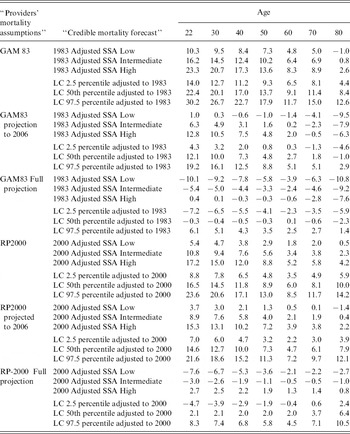
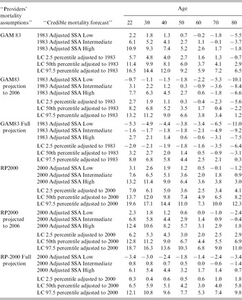
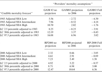
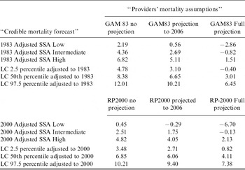
Tables 1(a) and (b) show the percentages by which projected benefit obligations of current plans would be understated for representative employees at selected ages; results for accumulated benefit obligations of frozen plans are almost identical and are not reported.Footnote 22 Although no direct comparison is possible, our methodology is similar to those of Watson Wyatt (Reference Watson2005) and Kessler (Reference Kessler2006), who calculates the change in annuity value at various ages resulting from switching from GAM83 to more recent tables with and without projection.Footnote 23 We use a 6.17% interest rate, the average used by surveyed pension plans to discount future pension obligations (Watson Wyatt, Reference Watson2004). We also have to combine information from the providers' mortality assumptions (which are annuitant mortality tables from previous dates) with the credible forecasts (which project population mortality beginning at the current date). We assume that male (female) annuitant mortality has declined and will continue to do so at the same percentage rate as past and projected declines in male (female) population mortality.Footnote 24
Percentage understatement of Projected Pension Obligations at Selected Ages – Male

Notes: The SSA cohort tables, for each alternative, are either adjusted by the ratio of GAM 1983 Basic mortality table to the 1983 SSA period table, or the ratio of RP2000 mortality table to the 2000 SSA period table. Mortality tables generated using Lee-Carter (LC) model are adjusted in the same way, but instead of GAM 1983 Basic we use GAM 1983 table. The assumed interest rate is 6.17%.
Percentage understatement of Projected Pension Obligations at Selected Ages – Female

Notes: The SSA cohort tables, for each alternative, are either adjusted by the ratio of GAM 1983 Basic mortality table to the 1983 SSA period table, or the ratio of RP2000 mortality table to the 2000 SSA period table. Mortality tables generated using Lee-Carter (LC) model are adjusted in the same way, but instead of GAM 1983 Basic we use GAM 1983 table. The assumed interest rate is 6.17%.
For males, the percentage understatements in Table 1(a) are dramatic at younger ages, reflecting the compounding of small mortality reductions over long periods of time. For example, the projected benefit obligation of a 22-year-old employee would be understated by 16.2% if the plan provider used GAM83, but instead mortality declined at the rate predicted by the SSA intermediate assumption. If mortality declined as predicted by the Lee–Carter model, the understatement reaches 22.4%. At age 60, the percentage understatements are much lower but still substantial – 6.4% and 9.1% respectively. The 10% margin in GAM83 is insufficient to offset the failure to project mortality improvements. The understatements for females (Table 1(b)) are smaller but still sizeable at younger ages. At age 22, the projected benefit obligation for a female employee would be understated by 6.1% under the SSA intermediate assumption and 11.4% under Lee–Carter. At age 60, the percentage understatements are 1.1% and 3.7%, respectively. At 70 and 80, projecting GAM83 results in male and female obligations that exceed those based on SSA intermediate forecasts since the 10% margin more than offsets any underestimation of the rate of mortality decline. In contrast, RP2000, when projected, produces obligations that closely match SSA projections. The increases are of the same order of magnitude as those reported by Antolin (Reference Antolin2007); he compared the present values of pension liabilities at various ages under the alternative assumptions that life expectancy either remained constant at 2005 levels, or increased at the rate of 1.2 years per decade as forecast by the OECD.
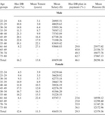
The dollar amounts of such obligations at younger ages are extremely small because employees have few years of service and because the eventual benefits are subject to substantial time discounting. The age and tenure-weighted average understatement of liabilities depends on the age, salary, and current and expected tenure of employees currently participating in DB plans. Table 2 reports relevant statistics obtained from the 2004 Survey of Consumer Finances for males and females. The great majority of DB participants are middle-aged and older, and tenure grows substantially with age. As expected, men are more likely to have a DB plan, have longer tenure in the job, and higher annual earnings than women.
Defined Benefit Participation, Tenure, and Salary by Age

Notes: Authors' calculations based on the Survey of Consumer Finances 2004. Percent with DB among all individuals age 22–64. Mean tenure and salary are conditional on having a DB plan.
Table 3 reports, separately for male and female employees, the understatement of projected benefit obligations weighted by age, duration of service, and salary, assuming that all employees stay until retirement at age 60. We assume a 6.17% interest rate as before, a 2.5% inflation rate, and 1.1% real salary growth.Footnote 25 The average is heavily weighted in favor of older workers, not only because they predominate in DB plans but also because they have greater DB wealth given that they have longer tenure and their pension liabilities are subject to shorter discounting to retirement.
Percentage understatement of Projected Pension Obligations – Male

Notes: Authors' calculations. Figures weighted by age, tenure and salary. The assumed interest rate is 6.17%, inflation rate=2.5%, and real salary growth=1.1%.
Percentage understatement of Projected Pension Obligations – Female

Notes: Authors' calculations. Figures weighted by age, tenure and salary. The assumed interest rate is 6.17%, inflation rate=2.5%, and real salary growth=1.1%.
The overall average understatements fall between the Table 1(a) and (b) values for ages 50 and 60. For males, the weighted projected benefit obligation is understated by 8.0% if the plan provider uses GAM83 and mortality declines at the rate predicted by the SSA intermediate assumption, and by 12.2% if it declines as predicted by the Lee–Carter model. If the plan provider projects mortality to 2006, the understatement almost disappears under SSA intermediate, offset by the 10% conservative margin in GAM83, but there remains a 3.4% understatement if mortality declines follow the Lee–Carter model. If the plan provider uses the RP2000 table without projection, the understatements are somewhat lower than those obtained from GAM83–4.6% if mortality follows the SSA intermediate forecast, and 8.7% if it follows Lee–Carter. They are somewhat higher than GAM83 if the tables are projected to 2006–2.9% and 6.9% respectively under the above assumptions, reflecting the smaller impact of projection on the more recent RP2000 table.
For females, the understatements of weighted projected benefit obligations are much lower, due to the smaller decline in mortality from 1983 to date. For example, the understatement is 4.4% if the plan provider uses GAM83 and mortality declines at the SSA intermediate rate, and 8.4% if it declines at the predicted Lee–Carter rate. The understatements are slightly lower if the provider projects mortality to 2006 or uses the RP2000 table.
3.3 Aggregate mortality risk in defined benefit pension plans
After evaluating the impact of biased forecasts of mortality improvements, we now consider the effect on a DB provider's pension liability of aggregate mortality risk – the risk that a putatively unbiased forecast of mortality turns out to be incorrect. In the case of a continuing plan, we calculate the annual mortality risk faced by the plan provider. We assume that the plan provider correctly calculates his projected benefit obligation using the Lee–Carter model. As above, we select values of a and k to match our 2005 estimate of annuitant mortality, which is obtained by multiplying the RP2000 mortality rates by the ratio of 2000 to 2005 mortality rates from SSA period mortality tables. We construct gender-specific cohort mortality tables using the Lee–Carter model.Footnote 26 We run Monte Carlo simulations by drawing a realization of the e t term in equation (2) each year. The pension provider then revises the forecasts of k for all future years accordingly and updates the calculation of projected benefit obligation.Footnote 27
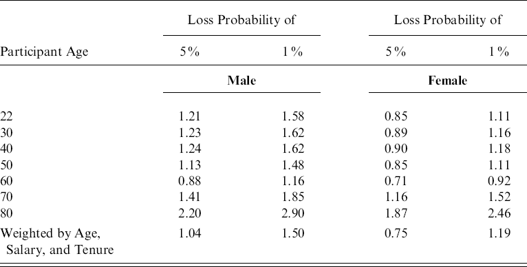
Table 4 reports our results. For 22-year-old male (female) employees, there is, in any year, a 5% probability that the projected benefit obligation increases by 1.21% (0.85%) or more. There is a 1% probability that it increases by 1.58% (1.11%) or more. The 5% and 1% risks for men peak at 1.24 and 1.62% at age 40, decline to 0.88 and 1.16% by age 60, and then rise again at older ages.Footnote 28 The age, tenure, and salary-weighted averages of these 5% and 1% risks are 1.04 and 1.50%, respectively. We view this level of risk as being moderate overall, while it is small in relation to (say) the risk of investing in equities.
Annual Aggregate Mortality Risk in Continuing Plans, by Gender
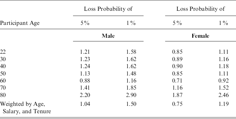
Notes: Authors' calculations. Annual aggregate mortality risk is as percentage of projected benefit obligations. Interest rate=6.17%. Results are based on Lee-Carter estimates.
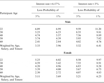
In the case of a frozen plan, we calculate the present value of the risk to pension assets over the entire period during which the assets are spent down, and not just the annual risk that was just reported for continuing plans. We calculate the plan's accumulated benefit obligation, assuming that mortality follows the predictions of the Lee–Carter model, and then run Monte Carlo simulations, noting the present value of the payments in each simulation. Table 5 reports our results. For 22-year-old male employees, there is a 5% probability that the accumulated benefit obligation exceeds the predicted amount by 6.1% or more and a 1% probability that it exceeds it by 7.0% or more. These values decline with age, since older employees have shorter remaining life expectancies and hence less risk of much lower realized mortality than predicted. For 60-year-old employees, there is a 5% (1%) probability that the accumulated benefit obligation exceeds the predicted amount by 2.4% (2.8%) or more.
Lifetime Aggregate Mortality Risk in Frozen Plans, by Gender

Notes: Authors' calculations based on Lee-Carter estimates. Aggregate mortality risk as percentage of accumulated benefit obligations.
The results are quite sensitive to interest rates because payments in the distant future, which are forecasted with less certainty, are discounted much more heavily at higher interest rates. To illustrate, if instead of 6.17%, we use an interest rate of 3%, as might be appropriate for a plan providing inflation-protected benefits, the 5% and 1% probabilities at age 60 are 4.0 and 4.8% respectively. For the weighted accumulated benefit obligations of male employees, the 5% and 1% probabilities are 3.3 and 4.0% at a 6.17% interest rate and 5.3 and 6.4% at a 3% interest rate. The respective numbers are slightly lower for female employees.
Defined benefit pensions carry greater aggregate mortality risk than immediate voluntary annuities because a greater proportion of the payments lie in the more distant future, when there is greater uncertainty as to mortality rates. At older ages, the aggregate mortality risk converges to that faced by annuity providers (Friedberg and Webb, Reference Friedberg and Anthony2007), as the pension deferral period approaches zero.
3.4 The magnitude of the aggregate mortality risk faced by S&P 500 companies
Most S&P 500 companies – 74.2% of the total – offer DB pension plans and so are exposed to aggregate mortality risk through their pension plans. Credit Suisse First Boston (2006) compares the projected benefit obligations of S&P 500 companies with their market capitalizations. Projected benefit obligations total $1,488 billion at year end 2005, or 12.6% of the $11,941 billion S&P 500 market capitalization, so even substantial increases in projected benefit obligations would result in a total that was small in relation.
A minority of companies has very substantial exposure, though. General Motors had a market capitalization of $11,033 million and a projected benefit obligation of $105,175 million, yielding the most extreme ratio of one to the other in the S&P 500. Even a small increase in GM's pension obligations due to an aggregate mortality shock would be large in relation to its market capitalization.
4 Conclusions
Many households are insured against the risk of an uncertain lifespan through annuities provided by defined benefit pensions. The resulting mortality risk borne by companies that offer DB pension plans consists of idiosyncratic risk, since any particular pensioner may live longer than expected, and aggregate mortality risk, since pensioners may on average live longer than expected. We evaluate two components of aggregate mortality risk: the risk that DB plan providers are using a biased estimate of participant mortality, and the risk that the mortality experience of a provider is lower than that predicted by an unbiased estimate.
Although there is obviously disagreement over what might constitute an unbiased estimate, the two mortality tables (GAM83 and RP2000) commonly used by DB plan providers understate even current male longevity and substantially understate prospective male longevity, relative to forecasts made by both the Social Security Administration and the widely used Lee–Carter model. Pension providers basing their calculations of plan liabilities on either mortality table without projection would substantially understate those liabilities. The potential understatement for men could be in the range of 2.3 to 12.2%, given forecasts implicit in the SSA and Lee–Carter projections, respectively. In contrast, female longevity has improved by less, so the potential understatement is lower, ranging from 0.5 to 8.4%.
Even if plan providers were to base their calculations on unbiased forecasts of mortality, they are still exposed to the risk that the forecast proves to be incorrect. We calculate that this results in a 5% annual probability that the projected benefit obligation of a continuing plan would increase by at least 1.04%, and a 1% probability that it would increase by at least 1.50%.
Longevity bonds have been proposed as a mechanism to transfer aggregate mortality risk to capital markets. These can be structured so that payments are proportional to the number of survivors of a birth cohort. Although there have been a number of short-term bond issues, there has not to date been a single long-term bond of a type that might appeal to pension plans. The European Investment Bank attempted to launch such a bond, based on United Kingdom lives, but the issue was withdrawn. Cairns et al. (Reference Cairns, David, Paul and Kevin2005) report that the bond was to be issued at a discount of 20 basis points compared to equivalent non-mortality related bonds, based on mortality forecasts of the British Government Actuary's Department.
Some of our results may help explain the failure of the EIB bond. First, if pension plans really expect the mortality rates predicted by GAM83, then the longevity insurance offered by EIB-type bonds appears very expensive in relation to the amounts at risk. Second, our results show that, although aggregate mortality risk is sizeable, it is of a much smaller order of magnitude than, for example, asset return risk. Third, several people have suggested to us that the particular design of the EIB bond contributed to its unattractiveness. The issuers planned to transfer the aggregate mortality risk on to the reinsurance market, which might explain the relatively high price compared to what would be available through the wider capital market, according to our calculations.
A last possible explanation for the lack of demand for the EIB bond, and one that has very different implications about who bears the associated risk, is that aggregate mortality risk may have only a small effect on company values. This may be because investors differ in their taste for aggregate mortality risk, with only those most willing to bear it investing in firms sponsoring defined benefit plans. In this regard, future research may consider why sponsors of defined benefit pension plans use outdated mortality assumptions. Firms may be exploiting an information advantage over uninformed investors, or seeking to minimize current expenses in anticipation of future growth, when it will be easier to catch up on pension funding – though DB plans are most prevalent in mature industries.
Yet another possibility is that firms are trying to reduce Pension Benefit Guaranty Corporation (PBGC) premiums or maximize the value of the PBGC ‘put option’. As Treynor (Reference Treynor1977) pointed out, the opportunity to liquidate one's pension fund can be thought of as a put option held by employers. The put option provides the employer with a mortality option that pays out if mortality does not decline too rapidly. This option gained in value when the PBGC was created in 1974, allowing shareholders to put pension obligations off to the government, and the option has been increasingly exercised in very recent years. Of course, the put option against the PBGC can only be exercised in certain circumstances, for example bankruptcy. Although the price of this option, as reflected in PBGC premiums, varies with the plan's funding status, the variation in price does not fully reflect the variation in risk.Footnote 29 Moreover, the value of the option rises as aggregate mortality grows more uncertain. Purchasing insurance against aggregate mortality eliminates that part of the value of the put option that arises from aggregate mortality risk. To the extent that DB pension providers insure themselves through the PBGC, then, our calculations of the impact of aggregate mortality risk on pension liabilities are pertinent for taxpayers rather than shareholders.
Appendix: Calculating pension liability in respect of past service
Defined benefit pension plans typically relate pension benefits to final salary and years of service. Schieber (Reference Schieber, Gale, Shoven and Warshawsky2005) reports that, until the early 1980s, pension plans funded their benefits on the basis of the entry age normal cost method. This involved choosing a level percentage of salary that would be sufficient to fund the benefits, provided the plan's actuarial assumptions were met. But, the benefits in respect of service at younger ages will be paid in the distant future and will therefore be subject to substantial time discounting. In consequence, at younger ages the assets in the plan will significantly exceed the sponsor's obligation if the plan were to be shut down.
In the early 1980s, the Federal Accounting Standards Board introduced rules requiring the use of the projected unit credit (PUC) method for pension accounting purposes. Under this method, the pension liability equals the present value of the proportion of future benefits that relates to past service. The calculation takes into account projected wage increases. The American Academy of Actuaries (2004) provides an example. Joe is aged 55, earns $50,000 a year, has worked for 20 years, and is expected to retire at 65 on a salary of $75,000 a year. His pension benefit is 1% of salary per year of service. His expected pension is $22,500, of which $15,000 relates to past service. Under the PUC method, the pension liability equals the present value at age 55 of a pension of $15,000 a year starting at age 65. This is referred to for pension accounting purposes as the projected benefit obligation.
Under the PUC method, the accounting cost of providing a year's pension obligation increases with age. From an economic perspective, this method understates the firm's obligation at younger ages.
Participants in a terminated plan will not benefit from future salary increases, and the analogous measure of the firm's liability is the accumulated benefit obligation, the present value of benefits earned in respect of past service, but excluding any salary increases.