1. Introduction
In the oceans and atmosphere there are a range of physical mechanisms that cascade energy to smaller length scales. Together, they play a pivotal role in the global energy budget and are far from well understood. The direct energy cascade in geophysical flows can occur after the perturbations have reached a state of nonlinear equilibration through wave-mean-flow or wave-wave interactions. Alternatively, it has been postulated that energy can be transferred to smaller length scales through weaker linear instabilities that occur at higher wavenumbers compared with the most unstable mode. In this paper, we use the reduced gravity one-layer rotating shallow water (SW) model to study the dynamics of oceanic fronts in both the linear and nonlinear regimes using high-resolution numerical models. By considering two important case studies, we investigate the dynamics that are efficient in generating motions at the submesoscale.
The SW model describes geophysical fluids with strong ambient rotation and small aspect ratios (Pedlosky Reference Pedlosky1987). Shallow water theory is more versatile than simpler models, such as quasi-geostrophy (QG), in that it allows for a wide range of Rossby numbers and it admits layer depths that can vary significantly in magnitude and even vanish. Even though SW is computationally more expensive to solve than QG, it is used a great deal by the geophysical community since it gives us a relatively simple paradigm to explore rather complex motions; see Zeitlin (Reference Zeitlin2007) for a range of examples. One classical example is to study the interaction of slow vortical motions and fast gravity waves (Warn Reference Warn1986; Ford Reference Ford1994; Bartello Reference Bartello1995). However, numerical solution of this set of equations in the case of an outcropping/incropping front is more challenging, and many standard methods can become numerically unstable and fail.
Paldor (Reference Paldor1983), Killworth, Paldor & Stern (Reference Killworth, Paldor and Stern1984) and Boss, Paldor & Thompson (Reference Boss, Paldor and Thompson1996) explain how to deal with an outcropping in the context of a one- and a two-layer SW model in the case of an active surface layer. In the one-layer case, they state that one enforces the conservation of momentum and mass at the boundaries. This simplifies matters in that one does not need to do anything differently at the boundary of the fluid compared with the interior. With two active layers, where in the mean state the lower layer is motionless, the only difference is that they impose a condition at the outcropping such that the pressure in the lower layer exponentially decays away from the front. This has been demonstrated to work efficiently in the context of a linear stability analysis using a pseudo-spectral collocation method (Scherer & Zeitlin Reference Scherer and Zeitlin2008; Gula, Plougonven & Zeitlin Reference Gula, Plougonven and Zeitlin2009; Gula & Zeitlin Reference Gula and Zeitlin2010). In the context of bottom trapped flows, Teigen (Reference Teigen2011) and Teigen et al. (Reference Teigen, Nilsen, Skogseth, Gjevik and Beszcynska-Möller2011) looked at incroppings that can occur along steep shelves in coastal regions. There, they imposed no-normal flow in both layers at the location of the solid boundaries.
The pioneering work of Boss et al. (Reference Boss, Paldor and Thompson1996) compared the stability of a front with that of a jet with non-zero minimum depth and obtained some interesting results. First, they showed that there is a direct connection between the most unstable frontal SW mode and the corresponding unstable QG mode. This dispelled the myth that was widely held about whether these modes were non-QG in nature. Second, in addition to the classical long-wave QG instability (the most unstable mode), there are also ageostrophic short-wave baroclinic instabilities that occur due to a resonance between a gravity wave and a vortical wave. They claimed that both are observed in oceanic fronts, but it is not evident that the shorter-wave instability has been observed in oceanic data. Furthermore, they stated that the most unstable modes in question cannot exist in a one-layer model, but could only exist with two active layers. Dritschel & Vanneste (Reference Dritschel and Vanneste2006) demonstrated that the one-layer profile is in fact unstable due to an exponentially small growing instability.
To establish these findings, Boss et al. (Reference Boss, Paldor and Thompson1996) considered a surface layer with piecewise constant potential vorticity (PV). This is a popular approach that has also been used by others to study oceanic fronts (Iga Reference Iga1993, Reference Iga1999; Iga & Ikazaki Reference Iga and Ikazaki2000). What is peculiar about this choice is that the velocity profile is dependent on the mean depths far away from the front. Consequently, as the minimum depth vanishes the velocity profile changes shape and therefore the profiles differ much more than simply changing their minimum depths. In this work, we consider a geostrophic Bickley jet profile and examine a range of minimum depths. Since the velocity profile is always the same in each case we argue that this case study can better illustrate the effect of only changing the minimum depth. However, because these profiles do not have constant PV profiles we need to solve the problem numerically. We find that the case of vanishing layer depth requires very high spatial resolution because of the high-frequency structure of some of the unstable modes. We do this by first using a spectral collocation method to guess the frequencies of the modes and then a much finer finite difference method to correct the results (Irwin & Poulin Reference Irwin and Poulin2014). Even though we cannot find analytical solutions, the fact that the profiles are smooth makes them a very attractive paradigm in which to study the stability of observable oceanic currents.
Boss et al. (Reference Boss, Paldor and Thompson1996) also briefly discussed the case of a parabolic height profile, which we refer to as a parabolic double front, but this has since been investigated in great detail in Scherer & Zeitlin (Reference Scherer and Zeitlin2008). They determined that there was a range of instabilities and further illustrated some aspects of the nonlinear evolution of the primary and secondary instabilities. These instabilities were deemed to be due to a resonance of so-called frontal modes (Killworth et al. Reference Killworth, Paldor and Stern1984), and their work has since been extended into a two-layer model (Ribstein & Zeitlin Reference Ribstein and Zeitlin2013). Using similar methods, we illustrate a slightly wider range of unstable modes and show how they can be nicely categorized based on the number of nodes on each side of the current. We show that there is a doubling up of these modes that did not seem to be mentioned in the literature previously.
Furthermore, we present the nonlinear evolution of unstable modes to study the effect of vanishing layer depths. This employs a new higher-order finite volume method that uses a weighted essentially non-oscillatory (WENO) scheme for advection (Shu & Osher Reference Shu and Osher1988) combined with Zhang limiting (Zhang & Shu Reference Zhang and Shu2011) to preserve the order of accuracy of the method where possible. We are able to simulate a high spatial resolution in a reasonable amount of time due to the fact that the code is parallelized using the message passing interface (MPI) in both dimensions. We determine that gravity waves are radiated from the resulting vortices, as previously observed in Ford (Reference Ford1994). Moreover, by using a fine enough resolution we find that the elliptical rings that develop in the parabolic double front become unstable and create many small submesoscale features.
The structure of this paper is as follows. In § 2, we present the linear and nonlinear methods we use to investigate the stability of oceanic fronts. Then, in § 3, we study the linear stability and nonlinear evolution of the Bickley jet front and compare it with scenarios where the depths do not vanish. In § 4, we complete a similar analysis in the context of the parabolic double front for different Burger numbers. Section 5 analyses the characteristics of the nonlinear simulations in some detail. Finally, in § 6, we conclude our findings.
2. Numerical techniques
We begin by considering a reduced gravity SW model in which the top layer overlies a deep quiescent lower layer. We consider two different jet profiles in the upper layer and consider both outcropping and non-outcropping fronts. In this set-up, the nonlinear governing equations are
 $$\begin{eqnarray}\displaystyle & \displaystyle \frac{\text{D}\boldsymbol{u}}{\text{D}t}+f\hat{\boldsymbol{k}}\times \boldsymbol{u}=g^{\prime }\boldsymbol{{\rm\nabla}}{\it\eta}, & \displaystyle\end{eqnarray}$$
 $$\begin{eqnarray}\displaystyle & \displaystyle \frac{\text{D}h}{\text{D}t}+h\boldsymbol{{\rm\nabla}}\boldsymbol{\cdot }\boldsymbol{u}=0. & \displaystyle\end{eqnarray}$$
 $\boldsymbol{u}=(u,v)$
to denote the horizontal velocity;
 $h$
is the total depth of the layer,
 $f$
is the Coriolis parameter,
 $\hat{\boldsymbol{k}}$
is the unit vector in the
 $z$
direction and
 $g^{\prime }$
is the reduced gravity. It should be noted that
 ${\it\eta}$
is the interfacial height between the active surface layer and the passive lower layer. Using typical oceanic values, we take
 $g^{\prime }=0.02~\text{m}~\text{s}^{-2}$
and
 $f=10^{-4}~\text{s}^{-1}$
(Talley et al.
Reference Talley, Pickard, Emery and Swift2011).
2.1. Basic states
In this paper, we examine two different geostrophic velocity profiles. One correspond- ing to a Bickley jet front and the other to a parabolic double front. We choose the domain to be a periodic channel aligned in the
 $x$
direction with a meridional extent of
 $y\in [0,L]$
.
In the case of a Bickley jet, we define the layer depth and velocity to be
 $$\begin{eqnarray}\displaystyle & \displaystyle H(y)=75\tanh \left(\frac{-y+L/2}{L_{j}}\right)-(75+d), & \displaystyle\end{eqnarray}$$
 $$\begin{eqnarray}\displaystyle & \displaystyle U(y)=-\frac{g^{\prime }}{f}H_{y}, & \displaystyle\end{eqnarray}$$
 $d$
is the minimum depth of the layer and the parameter
 $L_{j}$
determines the width of the jet. Throughout, we assume
 $L_{j}=5~\text{km}$
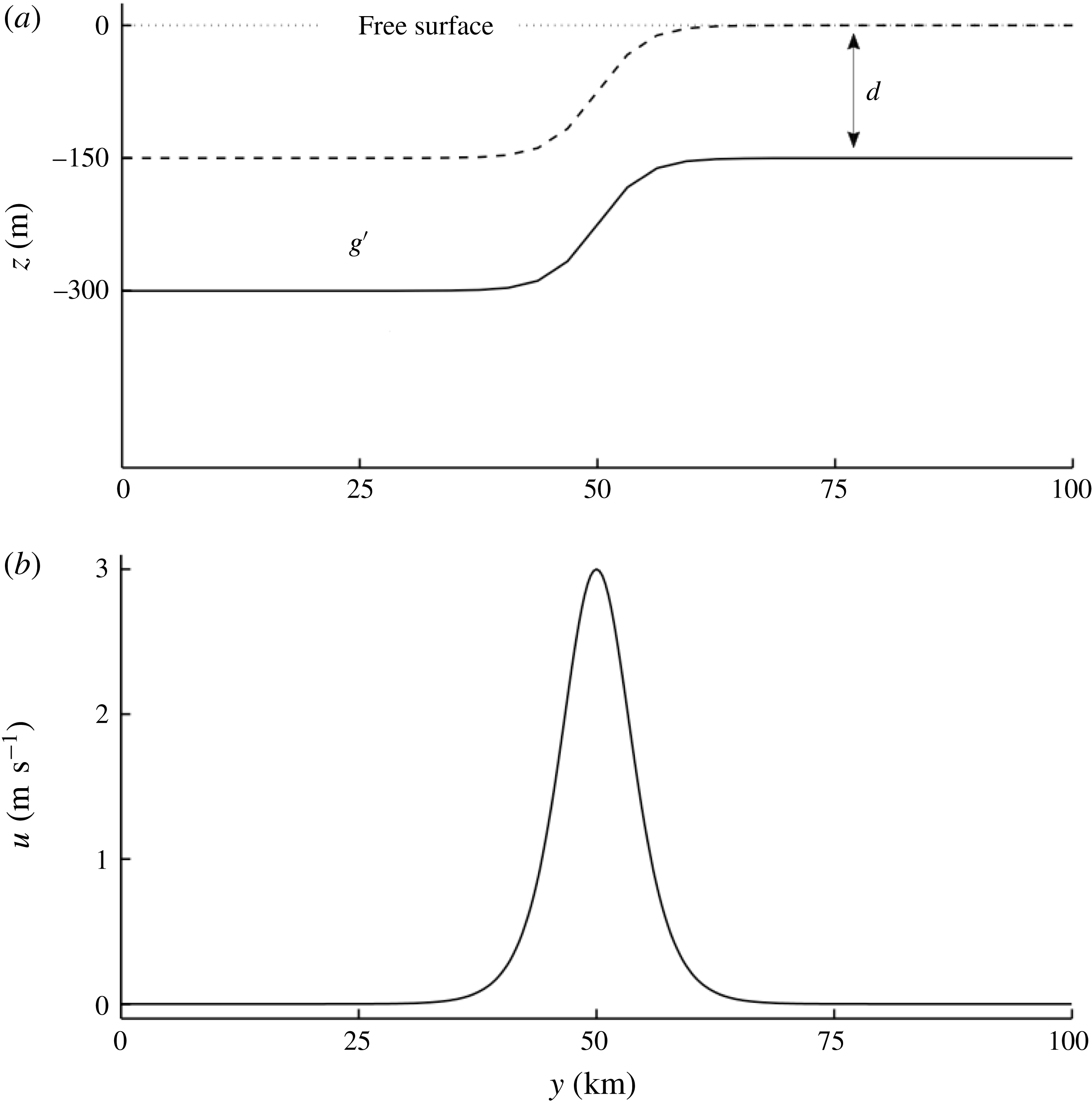
. Figure 1(a) depicts the depths of the layers in the two extreme cases and figure 1(b) shows the velocity profile that is common to each. It should be noted that the hyperbolic tangent profile is of fixed shape that can easily be shifted from a non-outcropping to an outcropping state simply by varying
 $d$
.
(a) The depth of the one-layer hyperbolic tangent profile in the two extreme cases: the solid line has a minimum depth of 150 m and the dashed line has a minimum depth of exactly 0 m. (b) The velocity profile for this entire family of profiles.

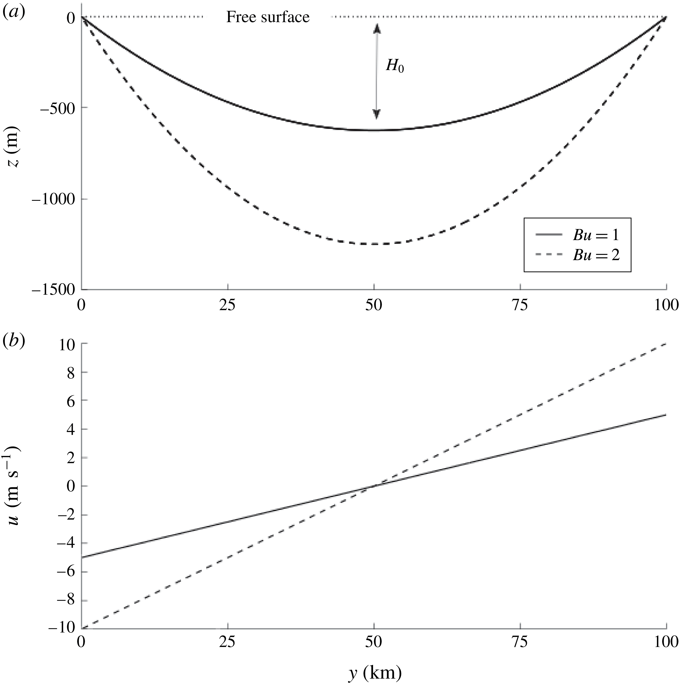
(a) The depth of the one-layer parabolic profile in the two extreme cases: the solid line has a maximum depth of 625 m and the dashed line has a maximum depth of exactly 1250 m. (b) The velocity profile in the two cases.

In the second case, our profile takes a parabolic form and is defined as
 $$\begin{eqnarray}\displaystyle & \displaystyle H(y)=\frac{H_{0}}{2}\left(1-4\left(\frac{y-L/2}{L}\right)^{2}\right), & \displaystyle\end{eqnarray}$$
 $$\begin{eqnarray}\displaystyle & \displaystyle U(y)=-\frac{g^{\prime }}{f}H_{y}. & \displaystyle\end{eqnarray}$$
 $Bu=4g^{\prime }H_{0}/(\,fL)^{2}$
. It should be noted that the factor of four is included to aid our later comparison with Scherer & Zeitlin (Reference Scherer and Zeitlin2008), where a domain of length
 $\tilde{L}=2L$
is used. Here,
 $H_{0}$
represents the maximum height of the dynamic layer as shown in figure 2(a). The interfacial displacements and velocities are shown in figures 2(a) and 2(b) respectively, for
 $Bu=1,2$
. It should be noticed that while the Bickley jet profile has an outcropping front only at the right-hand boundary, the parabolic double front outcrops at both edges of the domain.
2.2. Linear methods
To perform our linear stability analysis, we first assume a steady basic state satisfying
 $\{u,v,h\}=\{U(y),0,H(y)\}$
and, following Poulin & Flierl (Reference Poulin and Flierl2003), consider harmonic perturbations of the form
 $\{u^{\prime },v^{\prime },h^{\prime }\}=\{\hat{u} (y),\text{i}k\hat{v}(y),{\hat{h}}(y)\}\text{e}^{\text{i}k(x-ct)}$
. Given each of these profiles as our basic state, we can apply our normal mode decomposition for
 $u^{\prime }$
,
 $v^{\prime }$
and
 $h^{\prime }$
to the equations of motion and then linearize in order to obtain the following eigenvalue problem:
 $$\begin{eqnarray}\displaystyle & [U-c]\hat{u} +[U_{y}-f]\hat{v}+[g^{\prime }]{\hat{h}}=0, & \displaystyle\end{eqnarray}$$
 $$\begin{eqnarray}\displaystyle & [-f/k^{2}]\hat{u} +[U-c]\hat{v}+[(-g^{\prime }/k^{2})\partial _{y}]{\hat{h}}=0, & \displaystyle\end{eqnarray}$$
 $$\begin{eqnarray}\displaystyle & [H]\hat{u} +[H_{y}+H\partial _{y}]\hat{v}+[U-c]{\hat{h}}=0. & \displaystyle\end{eqnarray}$$
In order to solve this set of equations, we start by employing a spectral collocation method on a Chebyshev grid (Trefethen Reference Trefethen2000). While this is sufficient for the parabolic double front, we find that the Bickley jet front requires a very fine grid in order to achieve convergence. As this is computationally expensive when using dense Chebyshev differentiation matrices, we instead opt for a second-order finite difference technique due to the main advantage of being able to solve sparse matrices. In order to preserve some of the benefits of spectral accuracy, we use the Chebyshev method on a coarse grid first and then use our solution as a seed for the higher-resolution finite difference approach. One difference between our low-order method and that used in Irwin & Poulin (Reference Irwin and Poulin2014) is that we use a staggered C-grid. This proved to remove a class of spurious modes that otherwise persisted for zonal wavenumbers beyond a critical value.
2.3. Nonlinear methods
The nonlinear equations, (2.1) and (2.2), are solved numerically using a finite volume method. The advection in the momentum equations is discretized using a WENO algorithm on a staggered C-grid that maintains fifth-order accuracy where possible and a fourth-order centre differencing scheme for the pressure gradients. Fourth-order interpolations are also applied to the Coriolis terms due to the staggered grid. In the continuity equation we use a WENO method (Shu & Osher Reference Shu and Osher1988) with a Zhang limiter to ensure positivity throughout the simulation (Zhang & Shu Reference Zhang and Shu2011). The staggered velocity components coincide with the WENO interpolations and, therefore, we do not require the interpolation of velocity components when time-stepping the continuity equation. We use an SSP-RK3 time-stepping approach ubiquitous with the WENO methodology (Liu, Osher & Chan Reference Liu, Osher and Chan1994), which was originally developed by Shu & Osher (Reference Shu and Osher1988). To ensure numerical convergence, we conducted simulations on varying resolutions from
 $64^{2}$
to
 $1024^{2}$
by successive doubling of the resolution in the zonal and meridional directions. The increased resolution, coupled with the fast surface gravity waves, poses strict conditions on the time step. We use the MPI with our computational grid split in two dimensions, varying the processor count from
 $2$
to
 $64$
processors, and have ensured computational efficiency of the parallelization.
3. Bickley jet front
Our choice of the Bickley jet front depicted in figure 1 has several advantages over that presented in Boss et al. (Reference Boss, Paldor and Thompson1996): (1) as we change the minimum depth the velocity profile does not change, (2) both the height and the depth profiles are
 $C^{\infty }$
and (3) it seems to be a natural way to idealize oceanic flows rather than picking the PV profile. The issue that arises is that constant PV profiles are attractive for analytical treatment, but are not necessarily good idealizations of the real world and can cause problems in numerical methods because of kinks that tend to occur. Our analysis in this section will attempt to determine how the results of Boss et al. (Reference Boss, Paldor and Thompson1996) generalize to more realistic oceanic flows.
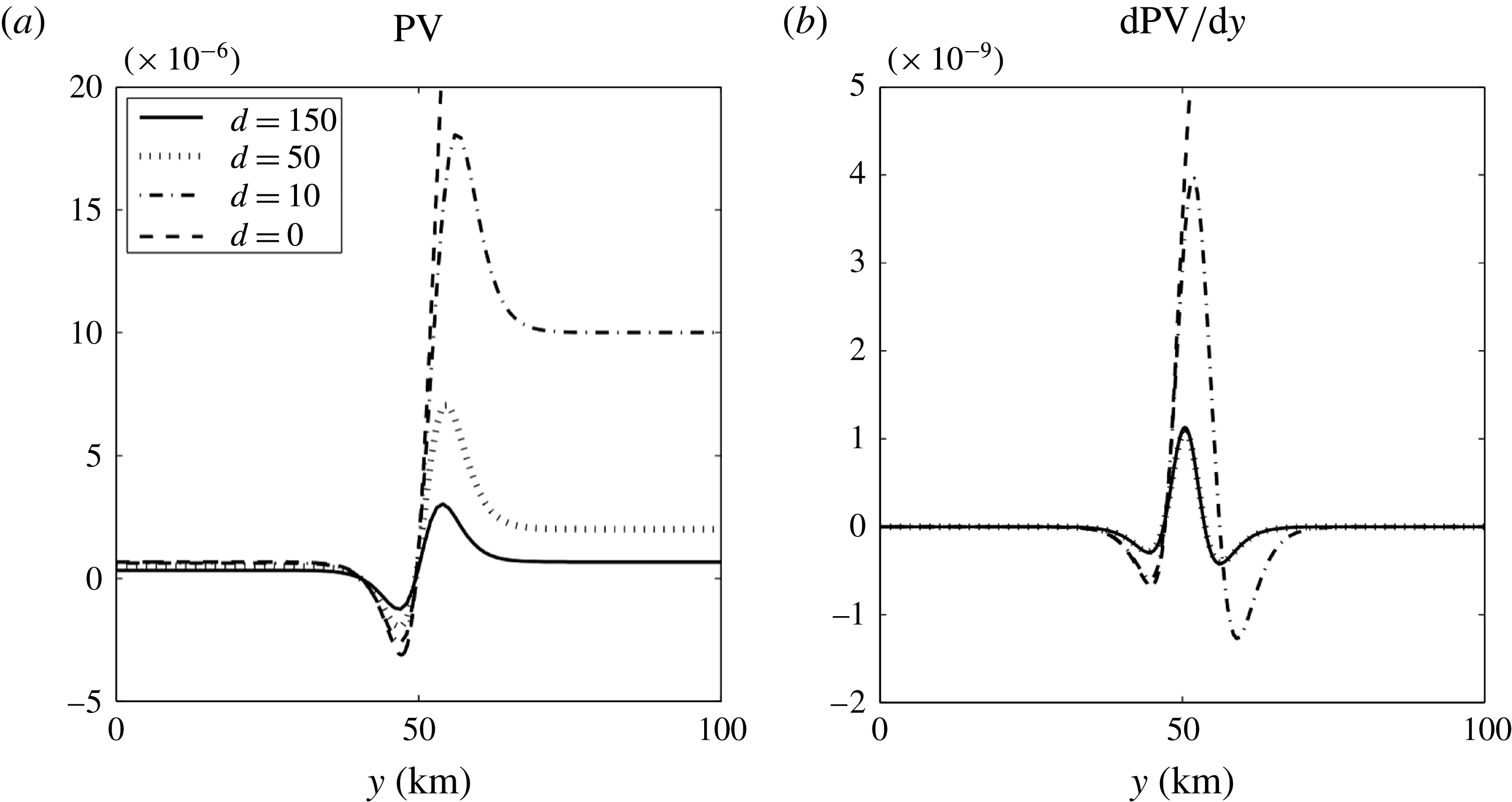
(a,b) The PV and the derivative of the PV for four different cases where the minimum depth is 150, 50, 10, 0 m. It is clear that the PV is negative in each of the cases and therefore the front is susceptible to inertial instability. Furthermore, the derivative of the PV changes sign at least once, which implies that it satisfies the criteria for BT instability.

3.1. Necessary conditions for instability
There are several necessary criteria for SW instability. Ripa (Reference Ripa1983) shows that these are related to (1) shear or barotropic (BT) instability (the gradient in the PV changes sign) (Poulin & Flierl Reference Poulin and Flierl2003) and (2) supersonic flow (the speed exceeds the gravity wave speed), but there is also the possibility of (3) inertial instability (the PV changes sign) (Bouchut, Ribstein & Zeitlin Reference Bouchut, Ribstein and Zeitlin2011). A good summary of this can be found in Ford (Reference Ford1993).
Figure 3(a) shows that the PV is negative for the four different profiles that are plotted, allowing for the possibility of an inertial instability. The corresponding figure 3(b) shows that typically the PV gradient changes sign twice, but when the layer depth vanishes this only happens once. This reduces the possibilities of instabilities and therefore can be interpreted as a stabilization in the flow; however, all profiles are susceptible to BT instability. It should be noted that there is an asymmetry that is evident in terms of the minimum value of this field, which is present because of the large Rossby number. This would not occur in the QG limit. Furthermore, the inertial instability could occur where the PV is negative, which is to the left of the jet axis. These criteria are quite valuable, but only suggest where instabilities could occur; they do not give us any information on the growth rates when they do occur. As we will demonstrate, numerical techniques are a very powerful means by which we can determine the stability of a hydrodynamic system. This allows us to determine the stability characteristics of the basic state with some degree of accuracy.
Boss et al. (Reference Boss, Paldor and Thompson1996) considered a profile with two regions of constant PV, and they state that the one-layer profiles are stable by Ripa’s two criteria. Clearly, the PV gradient is either zero or undefined in the middle of the domain and therefore does not violate Ripa’s first criterion concerning BT instability. However, they misinterpreted Ford (Reference Ford1993)’s explanation of the subsonic condition and deduced that it was also stable by the second condition (Jacques Vanneste (2014) personal communication). Subsequently, Dritschel & Vanneste (Reference Dritschel and Vanneste2006) showed that this is not in fact the case and that an exponential weak instability is possible. Since the one-layer continuous Bickley jet is susceptible to both barotropic and inertial instabilities, it is more unstable than the constant PV profile presented in Boss et al. (Reference Boss, Paldor and Thompson1996).
3.2. Linear stability analysis
We compute the growth rates of three different profiles where the minimum depth is
 $d=150,50,0~\text{m}$
and present the results in figure 4. We emphasize that the velocity profiles are identical in each case and therefore the differences that arise must be due entirely to the reduction in depth. The growth rates are calculated with a resolution of
 $N_{y}=1000$
and
 $N_{y}=20\,000$
on the Chebyshev and uniform grids respectively.
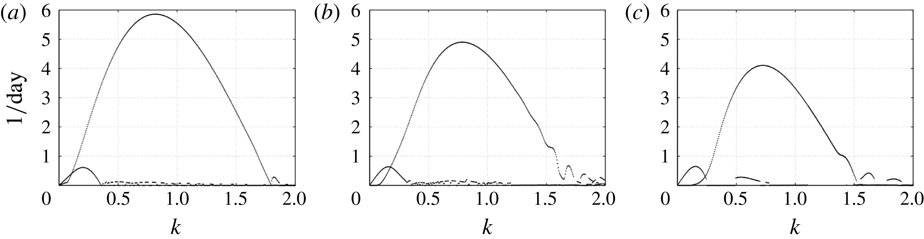
Plots of the growth rates for three different cases where the minimum depth is
 $d=150$
(a), 50 (b) and 0 m (c). The wavenumber is multiplied by
 $L_{j}=5~\text{km}$
, the width of the jet, and the growth rates are in units of per day.

In each of the three cases we observe that the most unstable mode has a typical growth curve that is an inverted U profile, which is well known to occur as a result of a BT instability in a Bickley jet (Flierl, Malanotte-Rizzoli & Zabusky Reference Flierl, Malanotte-Rizzoli and Zabusky1987; Poulin & Flierl Reference Poulin and Flierl2003; Perret, Dubos & Stegner Reference Perret, Dubos and Stegner2011) and was observed by Boss et al. (Reference Boss, Paldor and Thompson1996). As the minimum depth decreases, the maximum growth rate is reduced and the high and low wavenumbers on this curve are stabilized. At large scales, we also notice another mode of instability that is much weaker and is only marginally affected by a decrease in depth. Another consequence of reducing the minimum depth is to alter the stability at smaller scales. We see that the decay pattern of growth rates in the high-wavenumber regime varies in each case. For
 $d=150~\text{m}$
, the growth rate decreases linearly before it vanishes. For
 $d=50~\text{m}$
, the intermediate case, we see that oscillations develop at small scales. Finally, for the vanishing-layer case, we see that the modes seem to separate.
Contour plots of the perturbation height field that corresponds to the two most unstable modes for the Bickley jet profile for the case with
 $d=50~\text{m}$
. Panels (a–c) and (d–f) correspond to the most unstable and second most unstable modes respectively; (a,d), (b,e) and (c,f) are for
 $kL_{j}=0.1,0.8$
and
 $1.7$
respectively. The axes are in kilometres.

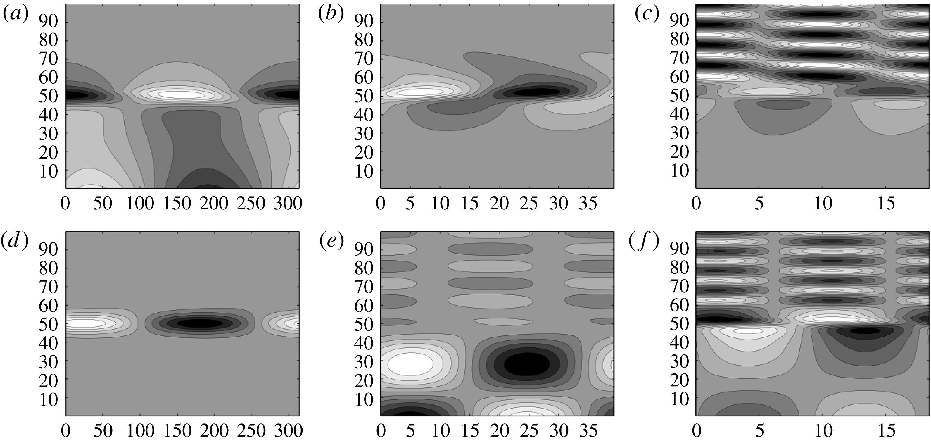
To better understand the nature of the unstable modes, we discuss the spatial structure of the two most unstable modes and how they are affected by the decrease in layer depth. In figure 5, we present the perturbation height field for different modes in the case with
 $d=50~\text{m}$
. Colour bars are not shown since the magnitudes of these linear waves are not important. Panels (a–c) correspond to the most unstable mode and panels (d–f) to the next most unstable mode; (a,d), (b,e) and (c,f) correspond to
 $kL_{j}=0.1,0.8$
and
 $1.7$
respectively. The most unstable mode over the range of wavenumbers is depicted in (b) and is a sinuous mode as typically appears in a Bickley jet, as recently discussed by Irwin & Poulin (Reference Irwin and Poulin2014). The mode in (d) is an extension of this mode, but at small enough wavenumbers that it is subdominant. It has a similar structure, but is more symmetric. We find that even when the layer depth vanishes, the most unstable mode is almost identical in terms of its spatial structure to what appears in (b).
The mode that dominates at large scales is illustrated in (a). This mode does have a strong structure in the centre of the channel where the PV gradient of the basic state is strongest, but it also has a trapped structure near the coast where the fluid layer is deepest. The deformation radius is largest in the deepest part of the domain, where it is approximately 17 m, and it subsequently decreases moving towards shallower waters. The lateral extent of the structures in the upper part of the domain is smaller than
 $17$
, which suggests that perhaps this mode of instability is a vortical Kelvin mode. In (e) at
 $kL_{j}=0.8$
, we see that there is a very weak mode with a growth rate of
 $0.11/\text{day}$
that has a strong wave structure in the deeper water and a relatively weaker wave structure of smaller meridional length scale in the shallower water. This is presumably due to gravity waves, but given the weakness of this mode it is not clear what physical significance it would have on the overall dynamics. In (c) at
 $kL_{j}=1.7$
, we have that the most unstable mode has a varicose structure near the centre, but then a highly oscillatory wave structure in the deeper waters. The secondary mode depicted in (f) looks very similar, but with a larger wave structure in the deeper waters. The growth rate of this mode is extremely weak at
 $0.01/\text{day}$
. It is important to state that the model structure indicated in (c) typifies the branch of the most unstable mode with
 $kL_{j}$
larger than
 $1.3$
. That is to say that the peak is well described by the classical sinuous mode, but at small enough length scales it changes. This is again in contrast to Boss et al. (Reference Boss, Paldor and Thompson1996), who did not find that the modes changed significantly throughout the main branch of instability.
In figure 4, we also see the existence of subdominant modes that appear predominantly in the
 $k=0.5$
to
 $k=1$
range. For the
 $d=150,50~\text{m}$
cases these are very weak compared with the primary instability peaks, and the lack of smoothness in the curves indicates that they are not sufficiently well resolved. However, when
 $d=0~\text{m}$
the growth rates are stronger and convergence is more readily achieved. This indicates that a decrease in minimum depth favours the generation of these secondary modes. We note a shortcoming of our numerical approach in that the curve starts abruptly at approximately
 $k=0.5$
. One could resolve this by implementing multiple seed solutions for the finite difference algorithm; however, given the small growth rates of these modes, they are unlikely to be significant in an oceanic context.
Plots of the perturbation height field that corresponds to the most unstable mode for the Bickley jet profile at
 $kL_{j}=1.7$
. Panels (a,c) and (b,d) are for
 $d=0,1~\text{m}$
respectively; (a,b) show the entire mode whereas (c,d) show a closeup around where the solution changes rapidly. The axes are in kilometres.

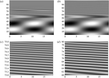
Next, we explore the nature of the small-scale linear instabilities in the regime where the minimum layer depths vanish or nearly vanish. In figure 6, we plot the height field of the most unstable mode using pcolor for
 $d=0,1~\text{m}$
in (a,c) and (b,d) respectively; (a,b) depict the entire mode, and we see that these modes have a Poincaré-like structure in the bottom half of the domain and this does not change significantly in the two panels. However, we find that the solution in the shallower water has a very high meridional variability. In the case with
 $d=1~\text{m}$
, it extends to the solid wall, but in the case of vanishing layer depth, it levels out before the wall. In panels (c,d) we plot closeups of the fields in panels (a,b). It should be noted that in the
 $d=0,1~\text{m}$
scenarios the meridional wavelength changes from approximately
 $200~\text{m}$
to
 $2~\text{km}$
. We emphasize that for the finite difference method these are well-resolved spatial structures with over
 $10$
grid points per crest. The spectral method that we have used cannot resolve the vanishing layer depth, which might be the explanation of why so many spurious modes appear and why they increase in growth rate with increasing wavenumber.
To test the effect of imposing or not imposing no-normal flow boundary conditions, we only needed to change the boundary condition at
 $y=L$
. We recall that the depth only vanishes at the boundary on the top. We found that whether we used a high-order spectral collocation method on a Chebyshev grid or a low-order finite difference method, both reproduced virtually identical growth rates and spatial structure. This brings us to conclude that the lack of difference is because of the nature of the basic state. The height and velocity fields decay exponentially on approaching
 $y=L$
. Therefore, the perturbation necessarily must vanish as well. It is because the perturbation is negligible near the vanishing boundary that our results are independent of what boundary conditions we impose. We will find in the next section that when we have a frontal mode that does not vanish rapidly enough near the boundary, there is a strong dependence on the choice of boundary conditions.
3.3. Nonlinear simulations
We investigated the nonlinear evolution of the Bickley jet profile with
 $d=150,0~\text{m}$
for a variety of spatial resolutions:
 $64^{2},128^{2},256^{2},512^{2},1024^{2}$
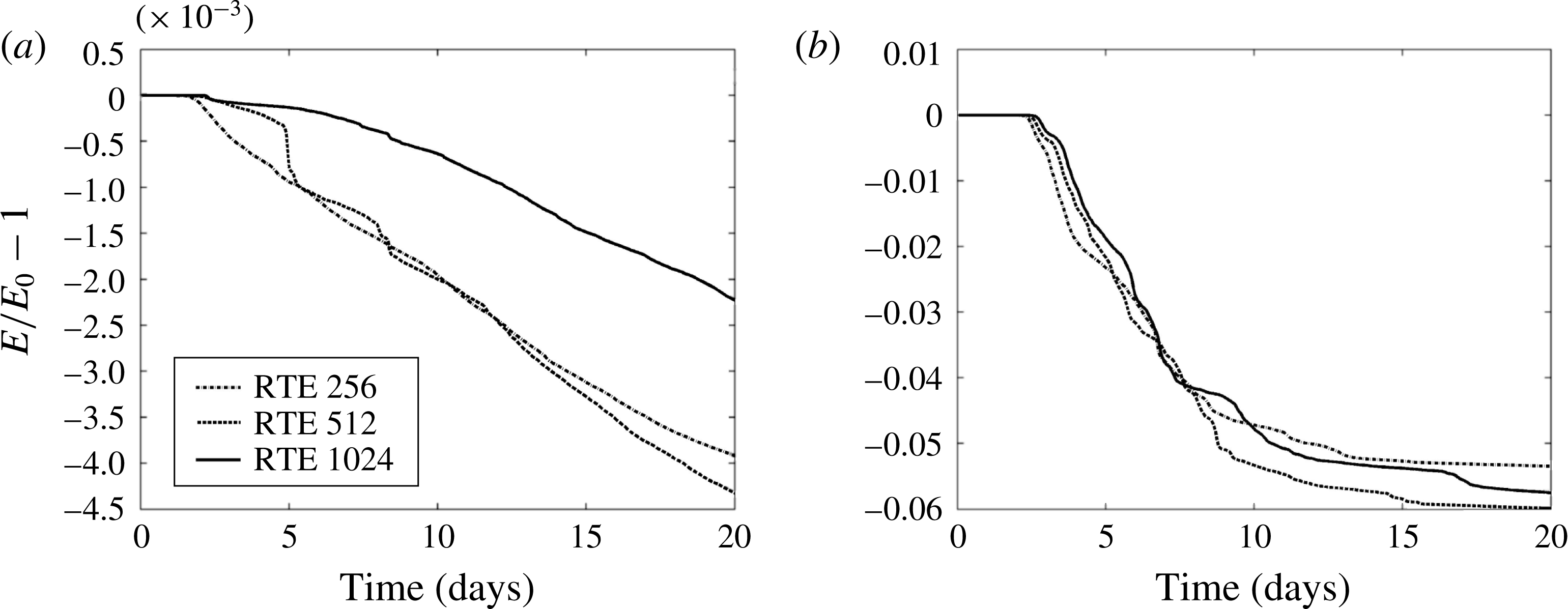
. In all cases the initial conditions are chosen to be our basic state (either a Bickley jet or a parabolic front) with white random Gaussian noise superimposed onto the height field which is several orders of magnitude smaller than the basic state itself. The relative error in the energy is plotted for the three finest resolutions in figure 7. Figure 7(a) indicates that for a simulation with a relatively deep minimum depth, the total energy is conserved within a fraction of a percent over the time span that it takes for nonlinear equilibration to occur (approximately 20 days). This is in contrast to the frontal regime, depicted in figure 7(b), where we see that even the finest-resolution calculation does not conserve energy nearly as well. Over the first few days, when the perturbations are very small, the energy is nearly conserved in all of the cases. However, after a few days the energy starts to decrease, and this corresponds to when the perturbations start to mature. The finest-resolution calculation does the best job early on in conserving energy, and after six days approximately 2 % of the energy is dissipated in the vanishing-depth test case. Subsequently, we have large meanders in the jet, and this corresponds to significant and rapid dissipation of energy. In fact, the finest-resolution calculation eventually dissipates its energy more than almost all of the simulations except for the very coarsest (approximately 6 %).
Plots of the relative error in the total energy in the Bickley jet profile with
 $d=150~\text{m}$
(a, total energy non-vanishing test case) and
 $d=0~\text{m}$
(b, total energy vanishing test case) from the nonlinear simulations over the first
 $20$
days for a variety of spatial resolutions.

This indicates that the regime of exponential growth is well captured by the numerical methods and an increase in resolution is advantageous to conserve energy for early times. However, after the stage of nonlinear equilibration, many vortical structures have formed, and they interact with each other creating a rather turbulent two-dimensional field. It is due to the dynamics at the front that the motion is dissipative, presumably due to the Zhang limiter that dissipates the flow to ensure positivity. We do not claim that this reduced gravity SW model is capturing precisely the correct physics of the ocean at a front, but it is known that fronts dissipate energy preferentially more than other regions of the ocean (Capet et al. Reference Capet, McWilliams, Molemaker and Shchepetkin2008a ,Reference Capet, McWilliams, Molemaker and Shchepetkin b ,Reference Capet, McWilliams, Molemaker and Shchepetkin c ), and at least this feature is well captured in our relatively simple model. Further details can be found in the supplementary materials provided at http://dx.doi.org/10.1017/jfm.2015.640, which contain animations of the fluid depth, vorticity and divergence of mass flux for all the numerical simulations discussed in this paper.
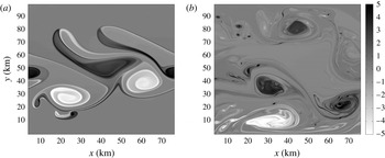
In figure 8(a,b), we present the vorticity field of the Bickley jet simulation with
 $d=150~\text{m}$
at days
 $2.87$
and
 $6.90$
. This is similar to what has been previously found in Poulin & Flierl (Reference Poulin and Flierl2003) and is presented as a reference simulation. However, even in this case there are some differences because of the relative shallowness of our parameters. In (a), we see that the vortex street is starting to develop and there are dipoles that are ejected on the bottom and top, but they have different shapes because of the different ambient depths. At later times, we see that the flow is dominated by a large dipole near the bottom boundary and some smaller-scale features.
Plots of the vorticity from the numerical simulation of the nonlinear evolution of the Bickley jet profile with non-vanishing layer depth. (a) The evolution after
 $2.87$
days; (b) the evolution at a later time of
 $6.90$
days.

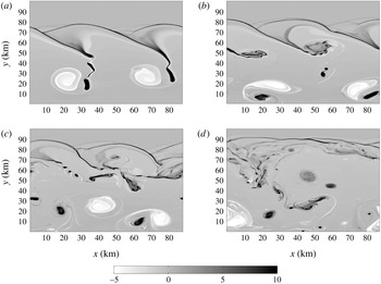
Plots of the vorticity from the numerical simulation of the nonlinear evolution of the Bickley jet profile with vanishing layer depth. (a–d) The evolution after
 $3.52$
,
 $3.98$
,
 $4.72$
and
 $6.39$
days respectively.

Figure 9 shows snapshots of the vorticity field of the Bickley jet simulation with
 $d=0~\text{m}$
at days
 $3.52,3.98,4.72$
and
 $6.39$
. These were chosen to illustrate certain interesting processes that occurred and to highlight some of the distinctions from the previous case we just mentioned. After the most unstable mode becomes sufficiently large, we see that the jet starts to meander. Figure 9(a) shows that large anticyclones have formed in the bottom of the domain and very thick cyclonic filaments have formed near the top, where the layer depth is shallow. In the intermediate region, we see that both cyclonic and anticyclonic fluid has been advected into deeper waters. This creates a long and narrow cyclonic region that becomes unstable and develops into several vortical components, with a very thin anticyclonic strip around it. Shortly afterwards, in (b), we see that the cyclonic fluid, which is left after the cyclones have pinched off, becomes unstable and forms a line of small anticyclones. These have lengths that are close to
 $1~\text{km}$
and therefore are in the submesoscale regime. Less than a day later, (c) shows how the thin cyclonic filaments destabilized into vortices once again. In the final snapshot, (d), we have that there is an abundance of cyclonic features in the shallower part of the domain. There are also small anticyclones that occur throughout the domain.
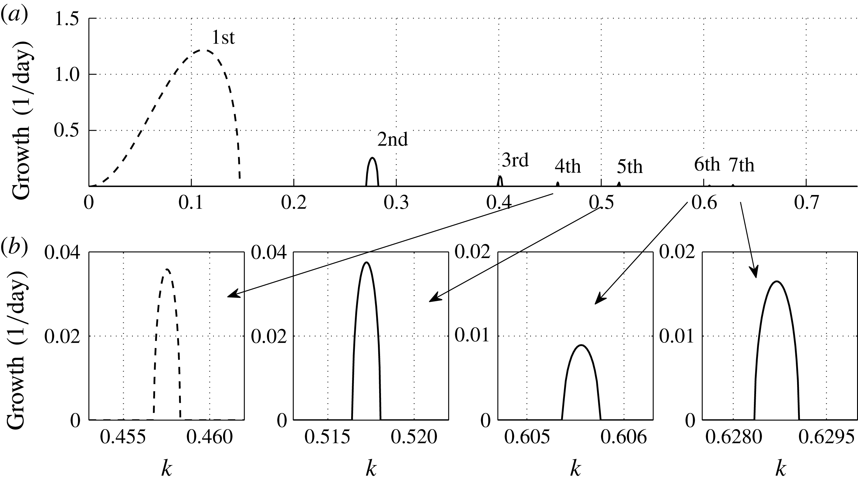
Plots of the growth rates for the parabolic case with
 $Bu=1$
. The wavenumber is multiplied by
 $L_{j}$
, the width of the parabola, and the growth rates are in units of per day. The dashed lines indicate a single unstable mode whereas the solid line denotes that there are two unstable modes.

From these two case studies, we deduce the following. In the case of vanishing (or perhaps even nearly vanishing) layer depth, we have that the vortex tube strength is much stronger, and this creates an abundance of thin cyclonic filaments that are most unstable. Therefore, there seem to be a greater number of smaller-scale features than what occurred in the case of a deeper minimum depth. Given that the size of these vortices is
 $O(1~\text{km})$
and their depth is less than 100 m, we expect that the SW approximation should still be valid. However, at these small scales one can expect that the effect of variable stratification could be more important. We recognize this and acknowledge that in a three-dimensional context there are bound to be some more interesting motions that develop. However, because the SW model is so much faster to solve numerically, this investigation is worthwhile to learn about the barotropic dynamics, which can be thought of as the leading-order behaviour. In future studies, we will investigate the dynamics of these fronts in a fully three-dimensional framework.
4. Parabolic double front
Figures 2(a) and 2(b) show the parabolic depth and linear velocity profiles respectively for
 $Bu=1,2$
. For our choice of parameters, the larger-Burger-number case reaches a depth of over
 $1~\text{km}$
and speeds of
 $10~\text{m}~\text{s}^{-1}$
, both of which are too large for oceanic flows. Thus, we focus primarily on the case with
 $Bu=1$
.
4.1. Linear analysis
The corresponding plots of the growth rates in the case with
 $Bu=1$
are presented in figure 10. This extends figure 2 of Scherer & Zeitlin (Reference Scherer and Zeitlin2008) for a wider range of wavenumbers to illustrate that many more unstable modes exist. We do not claim that these are the only ones that exist, there are almost certainly others, but presumably they are weaker because the growth rates tend to decay with the along-front wavenumber.
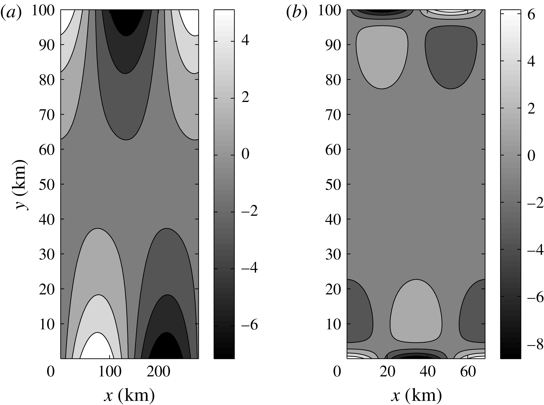
Contour plot of the perturbation height field that corresponds to (a) the first (1:1) and (b) the fourth (2:2) most unstable modes for the parabolic double front profile.

In figure 10(b), we show closeups of the growth rates of the different modes. The modes are labelled depending on the order in which they appear, and it is clear that the maximum growth rates of a given mode do not always decrease with increasing mode number; the seventh mode has a larger maximum growth rate than the sixth.
In figure 10, we plot the first and second unstable modes with a dashed and solid line respectively. Therefore, a dashed line indicates that there is only one unstable mode whereas the solid lines show that there are a pair of modes. The occurrence of some of these unstable modes in pairs was not previously mentioned in Scherer & Zeitlin (Reference Scherer and Zeitlin2008). Physically, this occurs because, as we will see, some of these modes are concentrated on one of the fronts. By symmetry, it is possible to have one on each front and hence we have pairs of modes.
The fact that many of these modes appear in pairs is of interest in terms of the nonlinear evolution of these instabilities. If, for example, we choose a channel geometry to be too small for the primary instability to grow, there will be two exponentially growing unstable modes that grow simultaneously. If the perturbations are initially very small in amplitude then each will grow independently, continuously extracting energy from the basic state. However, when we reach the stage of nonlinear equilibration, then we will have not only wave-mean flow interactions, but wave-wave interactions as well. This allows for a wider range of nonlinear interactions that can contribute more strongly to the cascade of energy through different wavenumbers.
To get a clearer understanding of the nature of these unstable modes, in figures 11 and 12 we present contour plots of the height fields of the various modes that we identified. Figure 11 shows the spatial structures of the first and fourth modes together because they are the only ones that do not appear in pairs. These modes are symmetric across the front and have mode-one and -two structures respectively. The waves along the two edges of the front are out of phase. We call these (1:1) and (2:2) to denote the numbers of modes we have at the top and bottom respectively.
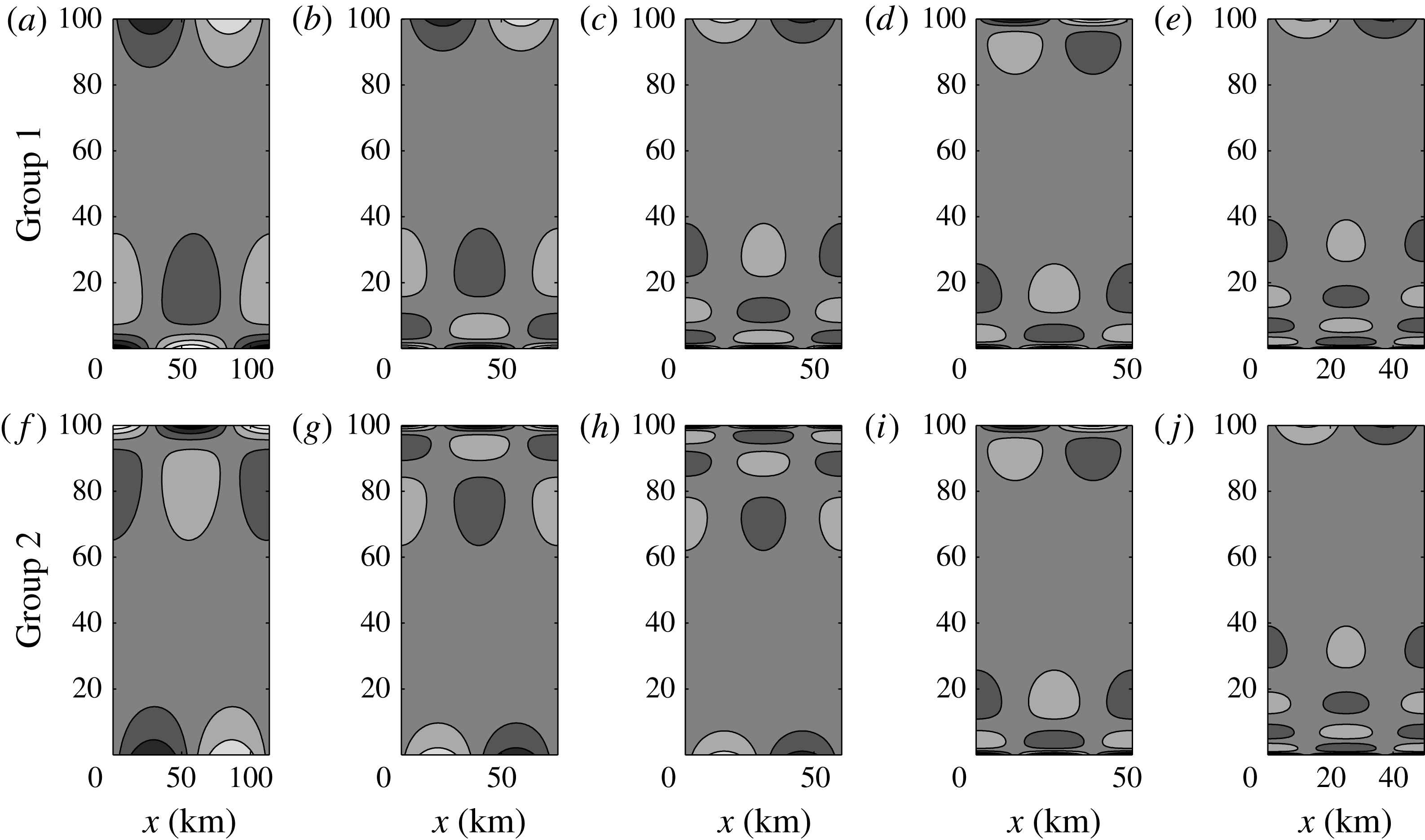
Figure 12 shows the same field for two groups of waves. Group one (two) has a higher mode structure on the top (bottom) edge of the front. The first three in each group have a mode-one structure on one edge and then two, three and four on the opposite edge. The seventh mode continues in this way with five nodes on one side, but the sixth mode deviates from the pattern in having two extrema on one side and three on the other. This in part explains why the sixth mode is weaker than the seventh because it has a higher modal structure, which has more difficulties in extracting energy from the front.
In the context of a parabolic double front, we have tested the imposition of no-normal flow boundary conditions or not and have determined that it makes a significant difference in the types of motion that can develop. Imposing walls at the front overconstrains the motion in that region such that frontal waves cannot exist. Certainly, this scenario can occur physically, but in that case the boundaries would prevent the most unstable modes from developing.
Contour plot of the perturbation height field that corresponds to the second (a) (1:2), (f) (2:1); third (b) (1:3), (g) (3:1); fifth (c) (1:4), (h) (4:1); sixth (d) (2:3), (i) (3:2); and seventh (e) (1:5), (j) (5:1) most unstable mode for the parabolic double front profile. It should be noted that panels (a–e) (panels f–j) have more (fewer) nodes on the bottom part of the domain.

4.2. Nonlinear simulations
In this section we reproduce a nonlinear calculation of the instability of a parabolic double front with
 $Bu=1$
, as previously shown in Scherer & Zeitlin (Reference Scherer and Zeitlin2008), but using our newly developed code with a higher spatial resolution. The basic state is perturbed with a random perturbation of very small amplitude. The amplitude is
 $0.1\,\%$
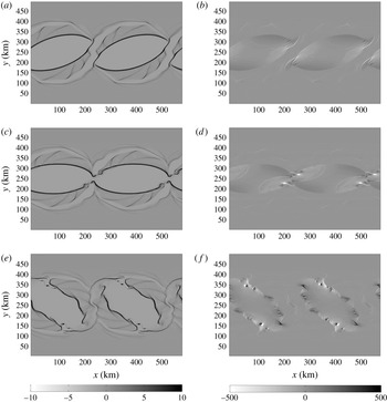
of the size of the background flow times a Gaussian random variable. Figure 13 plots the results of the numerical simulation of the nonlinear evolution of the parabolic double front with
 $Bu=1$
. Panels (a,c,e) and (b,d,f) show the vorticity and divergence of mass flux respectively; (a,b), (c,d) and (e,f) correspond to days 12.64, 13.10 and 14.26 respectively. The motivation for showing the divergence of mass flux instead of simply the divergence of the horizontal velocity is in part because Ford (Reference Ford1993) argues that this is a better measure for the presence of gravity waves. Furthermore, it has the advantage of concentrating on the regions where the depth is non-zero.
Plots from the numerical simulation of the nonlinear evolution of the parabolic double front with
 $Bu=1$
. Panels (a,c,e) and (b,d,f) show the vorticity and divergence of mass flux respectively; (a,b), (c,d) and (e,f) correspond to days
 $12.50,12.78$
and
 $13.89$
respectively.

Early on, the most unstable mode begins to form and grows exponentially. By looking at the vorticity plots, we see that the vorticity is constant almost everywhere except for at the front where we have long narrow strips. These strips begin to roll up because of nonlinear processes. When they do, the edges of the anticyclones have a strong positive divergence of mass. On the opposite side of the head, we have a long narrow region of mass convergence and increasing depth. At day
 $10$
we see that the front has pinched off in two different locations and has formed anticyclonic rings, which can be thought of as idealizations of rings generated from western boundary currents (Olson Reference Olson1991). The stability of the circular analogue of these anticyclonic rings in the context of the two-layer SW model was discussed in some detail in Lahaye & Zeitlin (Reference Lahaye and Zeitlin2015).
By
 $12.7$
days, we find that the vortices have reattached but, before this happens, there are some interesting structures that develop. Because we are studying the same parameters as Scherer & Zeitlin (Reference Scherer and Zeitlin2008), we believe that this is due to the increase in numerical resolution that allows us to resolve smaller-scale features. We see that filaments of negative mass divergence separate from the vortex, and two of these structures from different vortices meet. At
 $12.59$
days, they actually overlap. Afterwards, they continue to follow the vortex, but there seem to be arcs that are generated inside the head of each vortex that are associated with gravity wave radiation inside the vortices. Upon close inspection, we have verified that these are very well-resolved features in our model. At this stage, the region of positive divergence is rather small, but an abundance of submesoscale features are apparent. As time evolves, we do see these arcs radiate inside the vortex, signifying gravity waves propagating through the vortices. The depth of these disturbances is
 $O(1~\text{m})$
, which is very shallow considering that the mean depth of the vortex is several hundred metres. Therefore, the propagation of these ripples should be well described by linear dynamics, and we have confirmed that this is indeed the case. Furthermore, there is no evidence of nonlinear steepening or shocks that develop.
Given that the elliptical ring is formed by day 10 and is destabilized by day 13, we deduce that the e-folding time of this instability is of the order of hours. This instability is much faster than the primary instability of the parabolic double front and generates submesoscale cyclones. These vortices then reintegrate to form a ring.
Viewing the vorticity profile at the same time indicates that the ring of vorticity goes through a substantial change. As the vortices detach and a wave propagates along the filament and they continue to rotate, the thin strips of vorticity separate, and by day
 $14$
we have many distinct filamentary structures on the perimeter of the vortex. In between there are small patches of regions with strong divergence or convergence. This can be interpreted as a mechanism of instability that has occurred on the vortices. It is of interest to address the details of this mechanism since it could be directly relevant to a better understanding of western boundary current rings, but it is beyond the scope of this work and will be investigated in future research. Throughout the evolution, we see that ripples of gravity waves are generated and interference patterns between them are generated from opposite parts of the vortex.
5. Analysis of nonlinear simulations
The three high-resolution nonlinear simulations that we have already presented have each revealed that the dynamics that arise due to the primary linear instability can generate two-dimensional turbulent flows. In this penultimate section, we tease out the impact of having a vanishing layer depth using several different diagnostics. This includes examining the spectral kinetic energy density and the probability density function (PDF) of vorticity and investigating the equilibrated state after nonlinear saturation.
5.1. Spectral kinetic energy density
In a turbulent flow it can be very useful to compute the spectral kinetic energy density since it reveals how the energy is partitioned at different length scales. This relies on the fact that the kinetic and potential energies in the three-dimensional models are quadratic quantities and therefore Parseval’s theory is easily applied (Frisch Reference Frisch1995). Since the kinetic energy in the SW model is cubic (Warn Reference Warn1986), we instead focus on computing the spectral kinetic energy density,
 $\mathscr{E}(k)$
, based on the sum of the square of the transforms of the horizontal velocities,
 $|\hat{u} |$
and
 $|\hat{v}|$
,
 $$\begin{eqnarray}\displaystyle \mathscr{E}(k)=\int _{0}^{2{\rm\pi}}\int _{k-\text{d}k/2}^{k+\text{d}k/2}|\hat{u} |^{2}+|\hat{v}|^{2}\,\text{d}A, & & \displaystyle\end{eqnarray}$$
where
 $k$
is the wavenumber and
 $\text{d}k$
is the width of a binned region in wavenumber space. This equation integrates azimuthally in spectral space to get a one-dimensional field, which follows traditional theory (Frisch Reference Frisch1995).
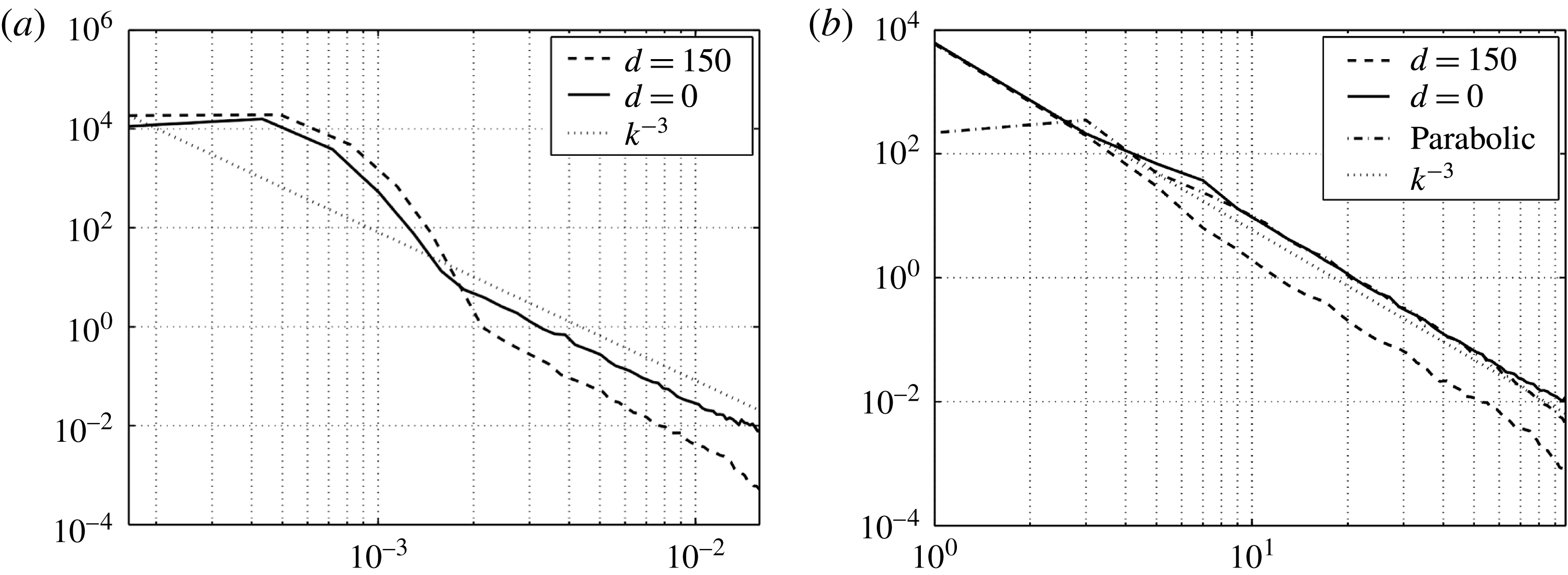
Plots of the spectral kinetic energy density (
 $m^{2}/s^{2}$
) as a function of wavenumber,
 $k$
, obtained from the three high-resolution numerical simulations presented in § 4. (a) The plots of the perturbation fields in the case of the two Bickley jet profiles with
 $d=0$
and
 $150~\text{m}$
compared with the reference line
 $k^{-3}$
. (b) A plot of the total fields, again compared with the reference line
 $k^{-3}$
.

Figure 14 presents the spectral kinetic energy density obtained from the three high-resolution numerical simulations presented in § 4. In (a) we depict the perturbation fields in the case of the two Bickley jet profiles with
 $d=0$
and
 $150~\text{m}$
, compared with the slope of
 $k^{-3}$
. Plotting the perturbation fields has the advantage of removing the initial condition, and therefore we know the kinetic energy density of the perturbation that arises due to the instability. Both curves have a bump at large scales at approximately
 $15~\text{km}$
and then have slopes that agree very well with the
 $k^{-3}$
reference line. Qualitatively they agree, but we clearly see that with
 $d=0$
there is relatively more energy at smaller scales. We estimate that it is larger by a factor of 5. This validates our previous statement that the simulations with vanishing layer depth tend to cascade more energy to the smaller scales. It would be of interest to study these instabilities in a primitive equation model that could more accurately describe the dynamics of the motion generated at the submesoscale. This will be pursued in future work.
Figure 14(b) shows the total fields in the three simulations, again compared with the slope of
 $-3$
. This shows that the two simulations with a basic state whose layer depth vanishes have more energy at the small scales. Perhaps coincidentally, we see that the slopes at the small length scales agree very well in the two cases where the layer depth vanishes. We did not plot the perturbation spectral energy density for the parabolic front because the WENO scheme diffused the basic state more in that case and it was not possible to get a clean comparison.
5.2. Distribution of vorticity
To sort out the asymmetries that develop in SW simulations due to vanishing layer depths, we compute the PDFs of the vorticity. Figure 15 plots these PDFs in the three nonlinear simulations considered. They are obtained by averaging over the second half of the simulations. The three panels correspond to Bickley jets with
 $d=150~\text{m}$
and
 $d=0~\text{m}$
and the parabolic front. The magnitudes of the positive and negative vorticities are depicted with solid and dashed lines respectively.
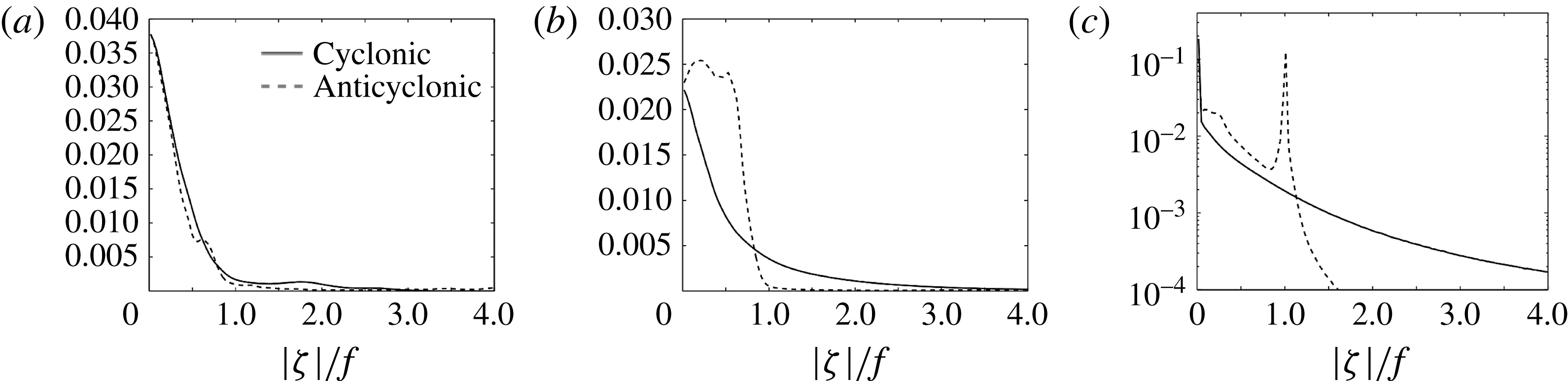
Plots of the PDF of vorticity in the three nonlinear simulations averaged over the second half of the simulations. The three panels correspond to Bickley jets with (a)
 $d=150~\text{m}$
and (b)
 $d=0~\text{m}$
and (c) the parabolic front. Positive and negative vorticity are depicted with solid and dashed lines respectively. The magnitudes of the vorticity values are normalized by the ambient rotation
 $|{\it\zeta}|/f$
.

Figure 15(a) shows that there are very slight differences between the cyclonic and anticyclonic components of the fluid, which is because the surface deformations are relatively small. We recall that if the anticyclonic fluid has a magnitude larger than 1 it is subject to inertial instabilities, which explains why the cyclonic tail is higher than the anticyclonic one.
The Bickley jet simulation with
 $d=0$
(b) shows a remarkable difference between the two curves. First, the anticyclonic fluid is almost entirely constrained between
 $0$
and
 $1$
and has a local maximum near
 $-f/4$
. If the relative vorticity decreases below
 $-f$
, inertial instabilities will develop and the net result is to reduce the magnitude of the ambient vorticity. In contrast, the cyclonic curve is monotonically decreasing and has a much wider tail since there is no analogue of inertial instability for positive vorticity. This reflects the fact that a large number of strong cyclonic vortices develop due to vortex tube stretching and possibly vortex merging.
The parabolic front case is quite different, and therefore we plot it with the
 $y$
-axis on a log scale. Initially, the vorticity is either
 $0$
or
 $-1$
. As the flow evolves, this changes significantly. There are still local maxima at
 $0$
and
 $-1$
, but the anticyclonic portion of the fluid has a wider range of magnitudes. The anticyclonic curve decays very rapidly, as a result of inertial instability.
5.3. Equilibrated mean flow
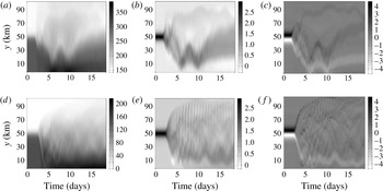
When the perturbations on a linearly unstable basic state reach large enough amplitudes they start to interact nonlinearly with the basic state. The nonlinear equilibration that occurs is very complex and hard to predict. In figure 16, we plot the temporal variation of the zonal average of the height (a,d), zonal velocity (b,e) and vorticity (c,f) fields for the two Bickley jet profiles. Early in each simulation the basic state is readily observed, but when the instability develops the mean state changes significantly. In each of the two simulations we see that the equilibrated state has a height field that is shallower and velocity and vorticity fields that are weaker after equilibration.
Plots of the temporal variation of the zonal average of the height (a,d), zonal velocity (b,e) and vorticity (c,f) fields for the two Bickley jet profiles. These are for the nonlinear simulations of the two Bickley jet profiles: (a–c) and (d–f) are for
 $d=0$
and
 $150~\text{m}$
respectively.

Two characteristics are readily observed from figure 16. First, in both cases the equilibrated states have a large variance. One could compute the mean over a range of times, but since the solution is in a two-dimensionally turbulent state we know that it is evolving and therefore we are not convinced this is a worthwhile endeavour. Second, the amount of variance is larger when the basic state has a vanishing layer depth. This is not surprising since, as we have previously seen, the smaller length scales are more energetic.
6. Conclusions
In this paper, we have revised the problem of how to model oceanic fronts in the context of the SW model and what kind of dynamics they produce. By studying a Bickley jet profile, which is a smooth extension of the constant PV profile in Boss et al. (Reference Boss, Paldor and Thompson1996), we are better able to study the effect of decreasing, and vanishing, layer depths since the velocity profile is the same in all cases. We find that the most unstable mode is essentially the sinuous mode in the Bickley jet. As the minimum layer depth decreases, we find that the growth rates of this mode decreases and it is stabilized at both high and low wavenumbers. Furthermore, we verified the existence of gravity–vortical modes, but find that they appear at both larger and smaller scales in comparison to the primary mode. Another difference from the work of Boss et al. (Reference Boss, Paldor and Thompson1996) is that we find these modes even with non-vanishing layer depths. However, given their weak growth rates it is unclear what impact they will have, if any, on oceanic dynamics.
We have also studied the classical parabolic double front. In the process, we have further explained the family of unstable modes previously observed by Scherer & Zeitlin (Reference Scherer and Zeitlin2008). We presented a wider range of wavenumbers, showing the spatial structure of the frontally trapped modes and how the asymmetric ones appear in pairs, and classify the modes based on the nodal structure along each boundary. We observe that the maximum growth rates of the different modes are not always decreasing monotonically with wavenumber, but that the growth rate also depends on the mode number.
We have performed some nonlinear simulations for the two different profiles in question using a new high-order finite volume method. We have determined the following characteristics of oceanic fronts: (1) the spectral kinetic energy density shows that the smaller scales are relatively more energetic in comparison to scenarios with deeper mean depths, (2) the PDF of the vorticity reveals that the magnitude of the anticyclonic vorticity is bounded above by
 $f$
, which is due to inertial instabilities that develop, (3) the parabolic front forms into rings that radiate gravity waves when the ellipses are aligned, which become unstable as they rotate, and (4) there is a stronger divergent field on the periphery of the ring which corresponds to relatively strong vertical motions. Of course, the reduced gravity SW model is limited in terms of what it can predict about these submesoscale motions, but our investigations illustrate some new dynamics that have not been previously appreciated and that we believe are relevant for oceanic fronts.
In future work, it will be of interest to study the dynamics of cold pools that exist along sloping topography that have incroppings instead of outcroppings (Poulin & Swaters Reference Poulin and Swaters1999; Teigen et al. Reference Teigen, Nilsen, Skogseth, Gjevik and Beszcynska-Möller2011). Furthermore, for both surface and bottom dwelling fronts, we will study these models in a three-dimensional non-hydrostatic model. This will allow us to determine more precisely what kinds of motions we expect to see in the oceans. Additionally, we should be able to better determine the limits of the SW formulation.
Acknowledgements
F.J.P. and M.C. would like to thank the National Sciences and Engineering Research Council of Canada and J.Y. would like to thank OGS for financial support during the research and writing of this paper. We would like to thank A. Stewart and the three reviewers for their comments which have helped us to revise this paper.
Supplementary movies
Supplementary movies are available at http://dx.doi.org/10.1017/jfm.2015.640.