

1. Introduction
The two decades after World War II represent an era of unprecedented growth in Europe's economic history, with GDP growth in Western European countries averaging 4.1 per cent and the highest level of convergence in history.Footnote 1 Assessing the factors behind this transformation is undoubtedly an interesting issue in economic history. A wide variety of explanations have been given for the remarkable behaviour of western economies during the Golden Age.Footnote 2 Most of them coincide in attributing a prominent role to the high investment rates recorded by western economies, but there have been few attempts to isolate the role played by the theoretical determinants of investment decisions and to relate them to the ‘exceptional historical conditions’ for technological transferability in post-war Europe.
One fundamental premise of this article is that such an increase in the investment rate needs to be studied within an appropriate theoretical framework. For this reason, this article presents an estimation of the Hall and Jorgenson investment equation for a group of three European countries (Germany, France and the United Kingdom) and the US during the Golden Age. The availability of homogeneous series of capital stocks has forced us to restrict the sample to four countries (O'Mahony Reference O'Mahony, van Ark and Crafts1996). Our objective is to verify the relative importance of the user cost of capital in the adjustment of European countries to a higher stock of capital. More specifically, we intend to highlight the importance of this factor when it comes to explaining the increase in the rate of investment in machinery and equipment. The user cost of capital displayed a distinct downward trend during the Golden Age that was mainly due to the drop in the relative price of machinery and equipment.
We believe that the trend in relative machinery and equipment prices could shed a great deal of light on the interpretation of the post-war economic growth. The reason is twofold. On the one hand, the decline in the relative price of machinery has been interpreted in the literature on economic growth as a sign of the embodiment of technological change in new equipment. Technology makes new equipment more efficient and less expensive with reference to other goods less exposed to technological improvements. On the other hand, the literature on the international diffusion of technology presents trade in capital goods as a way of spreading technological advances across countries. Exporters were normally the most innovative countries in the world and passed on their technological advances to their trading partners. Our premise is that after the World War II, European countries witnessed a boom in international trade. After three decades of tight restrictions on international trade, the increase in trade in capital goods saw American technology reach Europe. However, at the same time the increase in European commerce also allowed European countries to share their domestic improvements in technology. Hence the diffusion of technology advances through trade triggered a downturn in the relative price of machinery, which in turn registered higher rates of investment.
The first feature we document is the negative relationship between openness in the two decades after the war and the relative price of machinery in European countries. Trade liberalization increased the availability of foreign machinery that was cheaper (or of better quality) and increased the share of foreign goods in domestic investment, especially in European countries. The availability of foreign machinery could decrease the domestic price of machinery, which in turn increased the real investment rate as will be shown in the econometric estimation of the investment equation. The second feature that this article aims to highlight is that, thanks to technological change in the production of machinery and equipment, the cost of these goods dropped much more than the cost of structures, where technological change was much more modest. Additionally, as the literature on international comparative prices has shown, the cost of structures could benefit much less from trade liberalization than that of machinery and equipment because a larger share of structures consisted of non-traded goods (Kravis and Lipsey Reference Kravis and Lipsey1983).
The article is organized as follows. In the Section 2, we review some of the main explanations of the Golden Age and present an additional interpretation that stresses the importance of technological progress and the role of international trade in spreading it. In Section 3, we describe the evolution of relative capital prices and econometrically test the relationship between the decrease in the relative price of machinery and the upsurge in trade during the Golden Age. In Section 4 we econometrically estimate a capital stock adjustment formula. Section 5 concludes. Appendix 1 presents the data used and Appendix 2 the theoretical foundations of the investment equation.
2. Alternative interpretations of the Golden Age
2.1. A review of the literature
It is a well-known fact that European nations grew faster than ever during the two decades after World War II. This high growth has been explained in different ways. Most explanations highlight supply factors, while others emphasize conditions that created a special environment for demand stability that boosted investment and fostered economic growth. Supply explanations of the Golden Age could be summarized in three groups: the structural change hypothesis, the reconstruction effort thesis and the technological gap explanation.
The importance of structural change when explaining this high growth was first highlighted by Kindleberger (Reference Kindleberger1967). He argued that the availability of an elastic labour supply for manufacturing was the primary factor behind this economic growth. The abundance of labour kept wages low and promoted industrial peace. Temin (Reference Temin2002) recently reconsidered the structural change argument. In his opinion, after the war European countries resumed the industrialization that had been hindered during the drawn-out period encompassing the two wars and the Great Depression. During this 30-year period, international trade barriers prevented Europe from further specializing in manufacturing goods. As a result, the slowdown in industrialization created an imbalance after World War II characterized by excess labour in agriculture, bearing in mind the high level of income and how developed some European countries were. After World War II, international trade recovered, stimulating competition, which saw this imbalance disappear. Temin also deems the reduction of this imbalance as the end of the Golden Age.
The reconstruction effort thesis is another argument that has received widespread support. It was pioneered by Jánossy (Reference Jánossy1967). According to this argument, the countries that suffered the most damage during the war grew faster and these high growth rates correspond closely to the gap between actual production after the war shock and potential output taking into account a ‘normal’ growth path. The reason for rapid post-war growth was the disparity between the social capability for growth and its complement, physical stock of capital. Defenders of this argument tend to assign less importance to the destruction of physical capital during the war. Instead, they emphasize the role played by the imbalance between physical and human capital left by the war. In this sense Dumke (Reference Dumke1990) considers that the idea of ‘reconstruction’ refers to both the stock of physical capital and also to the removal of social, political and institutional barriers for growth.Footnote 3
The catch-up hypothesis has been considered a complementary explanation of the reconstruction effort made by some fast-growing OECD countries (Dumke Reference Dumke1990). But what distinguishes the catch-up gap from the reconstruction gap? In the reconstruction gap argument, disproportionate human and physical capital induced by the war was the factor that promoted growth. Meanwhile, in the catch-up argument, the factor that boosted economic growth was the distance between actual and potential output, which depended on the level of productivity in the leading country, the United States. Therefore, in the catch-up explanation the spread of international technology from the United States was a fundamental aspect when explaining growth.
A large number of papers based on the modern theory of economic growth have incorporated the ‘catch-up’ or the ‘productivity gap’ into the econometric regressions as an economic variable in order to explain economic growth or to measure the rate of convergence. This type of research is based on Solow's neoclassical model (exogenous technical progress), which forecast that all countries would converge to the same level of income and the same rate of growth. However, the empirical findings of the research carried out with various samples of countries and for different periods of time reveal that convergence is neither universal nor does it always occur at the same rate. The theory, consequently, has been reformulated and new explanatory variables included to capture countries' differing ability to grow, such as human capital (endogenous growth models).
As regards the Golden Age itself, the results of the empirical studies based on modern economic growth are quite misleading. Most fail to pay any special attention to the Golden Age as a specific period in which growth rates were exceptionally high. The reason is that they only date back to 1960 in order to better exploit the international data set available. Dowrick and Nguyen (Reference Dowrick and Nguyen1989), however, do analyse growth in OECD countries since 1950. Dumke (Reference Dumke1990) and Temin (Reference Temin2002) have also tested the idea of ‘catch-up’ against other specific factors more closely related to the Golden Age using cross-country regressions, but not exactly in the form of convergence or economic growth equations as in the literature quoted above. One aspect these studies have in common, however, is that they all confirm the productivity gap as an important part of growth. Moreover, this factor is always statistically significant in the studies that specifically refer to the Golden Age.
What else do economic historians say about the catch-up hypothesis and how this process occurred? Nelson and Wright (Reference Nelson and Wright1992), for example, highlight how technology invented and developed in the US over the last few decades of the nineteenth century spread widely across Europe after World War II. Up to that date, those technologies could not have been attained in Europe because they were particularly adapted to US resource endowments and market dimensions and also because protectionism had limited the transferability of American know-how to Europe. The US advantage in resource endowment (capital and natural resources), scale-intensive technologies and the so-called ‘high-tech’ industry widened the productivity gap between the US and European countries from the last quarter of the nineteenth century. After the war, the main pillars of the US advantage had been eroded because the European market had grown and natural resources were more readily available.
Moreover, the maintenance in Europe of what Abramovitz (Reference Abramovitz1986) called ‘social capabilities’ for growth was a crucial factor. These social capabilities were improved after the war by investing in education, consolidating more cooperative arrangements between state, firms and other interested parties and creating specific governmental institutions aimed at supporting technological change. European development of ‘social capabilities’ made leading technologies more ‘congruent’ with European resource endowment and market conditions (Abramovitz Reference Abramovitz1986).Footnote 4
The new attitude of policy-makers and market participants following the war played a special role in these changes (Eichengreen Reference Eichengreen, Crafts and Toniolo1996, p. 41). The lessons learnt from the interwar years period saw a new mentality emerge. New institutions were founded to promote a greater degree of economic integration and the expansion of both intra-European and international trade. The Marshall Plan aid, international cooperation within GATT, the Bretton Woods exchange system and afterwards, European economic integration through EFTA and the EC enabled international markets of goods and factors to become integrated, a situation that has been highlighted by various authors.Footnote 5
Apart from the structural change, the reconstruction effort and the catch-up hypothesis, other authors, including Eichengreen (Reference Eichengreen, Crafts and Toniolo1996), have identified high investment rates as the proximate source of post-war European growth that, moreover, makes it possible to explain differences in growth rates among countries. For the purposes of this article, it is worth paying special attention to the argument presented by Eichengreen (Reference Eichengreen, Crafts and Toniolo1996 and Reference Eichengreen2007). This author directs his attention towards the social and economic institutions founded during the Golden Age that created mechanisms to bind capitalists to investment and workers to wage moderation. On an international scale, agreements aimed at deregulating trade and reducing tariffs created new opportunities for investment and also to incorporate technological change, as the way had been paved to larger markets where countries could exploit their newly acquired comparative advantages. As a result, high investment rates were possible in a context of wage moderation and exceptional conditions for promoting exports boosted growth.
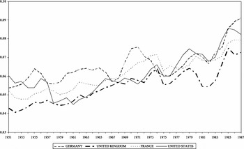
Figure 1 displays the upward trend in the real investment rate in machinery throughout the entire Golden Age. In Europe, technological innovation was in part embodied in the new machinery that needed to adopt American mass-production methods. In this article we explore some specific factors that help to explain these high investment rates, which also determined reconfiguration towards a new stock of capital.Footnote 6 The Hall and Jorgenson investment equation provides us with a suitable analytical framework to do so. In this model, reconfiguration towards a new optimal stock of capital depends positively on the expansion of demand and negatively on the changes in the user cost of capital. Demand expansion during the Golden Age appears to have received a great deal of attention, as some of the aforementioned interpretations have shown. Nevertheless, we would like to insist on the other component in the investment equation: the user cost of capital. The reason for this is that the latter is closely related to the specific technological change embodied in new capital goods. We consider that the high rates of investment were driven by declines in the user cost of capital, which was largely a consequence of the decrease in the relative price of machinery. This in turn was due to both factors: the embodiment of technological change in the production of new capital goods, which were to a large extent imported, and also to the boom in international trade after the war, which boosted capital goods imports.
Ratio of investment in machinery and equipment investment to GDP, 1951–87

2.2. An additional explanation of the Golden Age: the role of technological progress and trade of capital goods
Recent developments in growth accounting and growth theory consider that technological change made equipment less expensive, triggering increases in capital accumulation of equipment. For example, a growth-accounting exercise performed by Greenwood, Hercowitz and Krusell (Reference Greenwood, Hercowitz and Krusell1997) concluded that investment-specific technological change accounted for 60 per cent of output growth in the US during the post-war period and that the fall in residual productivity growth after the early 1970s could be explained by the opposite.
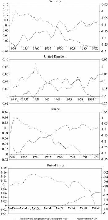
Figure 2 reproduces the real equipment price along with the ratio of the quantity of equipment in units of capital to GDP in consumption units (a similar plot appears in Greenwood, Hercowitz and Krusell (Reference Greenwood, Hercowitz and Krusell1997) and in Fisher (Reference Fisher2005) for the US). We can observe a general increase in the real investment rate in all four countries over the period 1948–73. In the subsequent period, 1973–87, this ratio became more stagnant for all the countries. Figure 2 also provides insight into why real investment prices might be important for understanding macroeconomic dynamics during the Golden Age: the real price decline coincides with a large increase in the relative quantity invested in equipment goods.Footnote 7
Real equipment prices against real investment in equipment

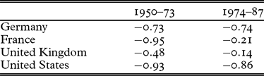
The relationship between the two variables plotted in Figure 2 is summarized in Table 1 through the coefficient of correlation. For 1948–73, this coefficient was −0.95 in the case of France, −0.73 for the UK and Germany and −0.93 for the US. This relationship was generally weaker in the subsequent period, 1973–87, when the value of the coefficient declined to −0.21 for France and −0.14 for the UK and remained almost unchanged for the US (−0.86) and Germany (−0.74), although all four countries buck this trend in relative machinery prices after 1974. These results could reveal a clear distinction between the Golden Age and the subsequent period of slowdown in productivity growth: the availability of technological change could be considered a clear stimulus for investment in the first period, while this assertion could not be made so strongly for the subsequent period.
Coefficient of correlation between real investment share and real machinery prices
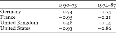
Source: See Figure 2.
But now we have two questions to answer: the first refers to how technological progress entered European countries and the second is why it was possible during the Golden Age, but not before. The reasons behind the decline in relative equipment prices could possibly be the same as in the US, the specific technological change in the production of investment goods that made capital goods less expensive and more attractive to investors. But some specific differences between the situation in the US and Europe should be noted. The first and most important difference is that European countries were followers. As has been seen in the previous section, the transfer of US technological change is the main argument used in the catch-up hypothesis. Access to foreign technology was able to be increased after the war because new international agreements provided new opportunities to reduce barriers to trade. As some authors have demonstrated, more open trade promoted growth during the post-war period.Footnote 8
International trade can be considered a channel for reaching foreign technology. The channels that have been most explored in the literature for measuring the dissemination of international technology are trade in capital and intermediate goodsFootnote 9 and R&D spillovers.Footnote 10 Verspagen (Reference Verspagen, Van Ark and Crafts1996, table 5.1, p. 219) provides data on R&D investment as a percentage of GDP for several countries since 1967. In that year, the US still appeared to be the clear technological leader in terms of R&D spending. The R&D investment rate of the other three countries (United Kingdom, Germany and France) was barely half that of the US. While the results presented by other authors suggest that we should not neglect the role of domestic innovation − especially if we consider that all the countries under study are among the main exporters of machinery and equipment in the world − it is worth indicating the technological superiority of the US up to as late as 1967.
Recent studies on international trade in capital goods (Eaton and Kortum Reference Eaton and Kortum2001) show that technological innovation used to be highly concentrated in the most advanced countries and thus technology advances spread from these countries to the rest of the world through trade in capital and intermediate goods. If international trade could transmit the benefits of technological advances across borders, the progress towards full capital goods market integration would lead to convergence in the relative price of capital goods. The reason is that lower-income countries will tend to buy equipment in the most advanced countries, where prices are lower in relative terms, because they are more efficient in the production of this kind of goods.
However, the fact that differences in the relative price of machinery goods persist between countries is a well-known economic fact. These differences are due to barriers that are natural to trade (such as distance, language, etc.) or to the presence of political barriers to trade, which fall under the umbrella of government policy. There is a vast amount of literature that emphasizes the role of economic policy and institutions in shaping the incentives to capital accumulation and development.Footnote 11
During the interwar period, numerous trade barriers were raised both inside Europe and also between Europe and the US that must have affected trade in capital goods (Collins and Williamson Reference Collins and Williamson2001). These barriers may have increased the cost of buying and using imported equipment and may have discouraged companies from acquiring foreign technology.Footnote 12 Therefore, convergence in relative machinery prices could be considered a positive consequence of the vigorous openness to foreign trade, the drop in transport costs and market integration that developed in Europe after World War II.
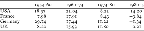
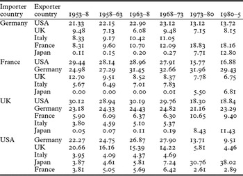
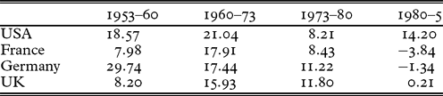
Table 2 presents the rates of growth of imports of machinery and equipment in real terms (as imports were expressed in current US dollars we have deflated them using the US durable goods price deflator). Machinery and equipment imports data have been collected from two sources. For the period 1953–62, data come from the United Nations Yearbook of International Trade Statistics (several issues). For the following years, data have been extracted from Feenstra et al. (Reference Feenstra, Lipsey, Deng, Ma and Mo2005). Trade in machinery grew at high rates throughout the entire Golden Age. After 1973, following the first oil shock, we can observe a decrease in the rate of growth that turned negative for some European countries after the second oil shock.
Rate of growth of machinery and equipment imports (annual accumulative rates, %)
Source: United Nations Yearbook of International Trade Statistics for the years 1953–62 and from Feenstra et al. (Reference Feenstra, Lipsey, Deng, Ma and Mo2005) for the years 1962–85.
Note: Imports expressed in current US dollars have been deflated for all the countries by the US durable goods deflator from the BEA.
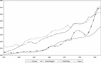
After World War II, equipment emerged as a highly traded good and, during the post-war years, imports of this kind of good boomed (see Table 2). As a consequence, the share of imported machinery in total investment increased, as can be observed in Figure 3, where the ratio of imports of capital goods over domestic investment is plotted.Footnote 13 Data referring to ‘machinery and equipment investment’ are expressed in terms of PPP-adjusted current international prices and are calculated as indicated in Appendix 1.
Share of machinery imports in machinery investment

As can be observed in Figure 3, the share of imported goods in domestic investment increased throughout the whole period for all four countries and the smallest proportion of foreign goods in domestic investment corresponds to the most developed country, the US. The importance of machinery imports as a percentage of domestic investment, at the beginning of the selected period, was below the levels estimated by Lee (Reference Lee1993) for OECD industrialized countries in conditions of free trade. Lee (Reference Lee1993) estimates that imports of machinery should represent approximately 28 per cent of domestic investment during the period 1960–85. Only at the end of the Golden Age had the average weight of imports in regard to domestic investment nearly reached the levels predicted by Lee (Reference Lee1993). This could be due to the gradual reduction of tariff barriers in developed countries through successive rounds of multilateral trade negotiations under GATT, and also to the creation, in 1957, of the European Economic Community.
For industrializing countries, Lee (Reference Lee1993) states that trade distortions caused by government tariff policies and exchange controls significantly lowered growth rates. Such policy action hampers supplies of imported inputs, thereby decreasing the productivity of capital accumulation. Quite the opposite occurred in industrial Europe during the Golden Age. The reduction of trade distortions made technologically superior capital goods more accessible and thus promoted investment and increased the share of imports within domestic investment, which had been artificially low since the interwar period.
Table 3 presents the country sources of machinery purchases. The main seller of machinery imports for the three European countries under consideration was the US. Imports from this country represent around 30 per cent of total equipment imports for France and the UK and around 22 per cent for Germany. It is also interesting to observe how the United States, despite distance, held a dominant position together with Germany.Footnote 14 This can be interpreted as an effect derived from US leadership in terms of technological progress. Although serious critical doubts have been postulated in the literature regarding the role of trade as a carrier of technology, the data compiled in this article emphasize the importance of American imports in European investment, and point to this country, the US, as one of the most outstanding exporters of technological progress to the most developed European countries.
Machinery and equipment imports by country of origin (% share in total imports)

Source: See Table 2.
Using the information presented as a basis, we can postulate some theories regarding the end of the Golden Age. We can see how the downturn in relative machinery prices was interrupted by the first oil shock and how prices remained stagnant following the second oil shock (see Figure 2). Moreover, real investment price stagnation coincided with flat investment rates. Does this mean that technological progress came to a halt? Bearing in mind the information to this respect, little can be concluded. There is widespread academic discussion regarding the technological origin of the slowdown in productivity growth in the second half of the 1970s and the 1980s, particularly in the United States.Footnote 15 However, one thing that remains crystal clear is that European trade in machinery deteriorated during this period. Growth in imports slumped drastically for all three European countries under study, all three even recording negative growth rates in the first half of the 1980s (France, −3.84%; Germany, −1.34% and the United Kingdom, 0.21%). Furthermore, trade worldwide underwent a remarkable change as the United States lost ground as an exporter of machinery, while Japan became steadily more important. This would imply that, if a significant amount of technological progress was imported, import difficulties that had arisen because of the first oil shock (the increase in transport costs, the instability in the international monetary market, the worsening in the real terms of trade of the industrialized countries, etc.) also hindered the transfer of technology and made it more difficult for the price of capital goods to decrease.
3. Convergence of the relative price of machinery during the Golden Age
In this section we will prove that the many facilities given to imports of machinery and equipment during the Golden Age favoured the access to less costly goods which were simultaneously more technologically advanced, and that this fact stimulated convergence in relative machinery prices throughout the period. With this purpose we will econometrically analyse the factors that determined the reduction in the relative price of machinery and will test the role played by the new international trade regime in the decrease of the relative price of machinery and equipment after World War II.
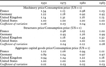
To do so, we first need to establish a cross-country benchmark comparison of the relative price of machinery, but also for other capital goods (structures and total capital goods). Table 4 includes some years for which this is possible: 1950, 1975, 1980 and 1985. For all these years, a purchasing-power parity price level is reported for investment components and for consumption for each country. The benchmark allows us to observe whether the price of capital relative to the price of consumption is high or low compared to the same ratio in the reference country (in this case the US). Thus, we can say something about the relative cost of capital goods between countries as well as over time by comparing successive benchmark years.
International comparative relative price level (US = 1, at different benchmark years)

Source: The 1950 benchmark data are from Gilbert and Kravis (Reference Gilbert and Kravis1954). The 1975 benchmark data are from Kravis, Heston and Summers (Reference Kravis, Heston and Summers1982). The 1980 benchmark data are from United Nations (1987). The 1985 benchmark data are from the United Nations and the Commission of the European Communities (1994).
In Table 4 we can see how the United States maintained the lowest level of relative price of machinery in 1950 and 1975, coinciding with its highest income level.Footnote 16 Throughout the period, the well-known convergence of European countries with regard to the US in terms of income levels corresponded to convergence in the relative price of machinery. Top-level prices in European countries tended to converge with the lowest level in the US. This convergence is measured by the coefficient of variation, which ranges from 0.06 in 1950 to 0.02 in 1985.
The negative association between income per capita and relative prices does not apply in the case of aggregate investment. In this case, a divergent trajectory can be observed for the relative prices of aggregate capital goods. The coefficient of variation runs from 0.01 in 1950 to 0.05 in 1980. The reason is that aggregate investment has a very significant non-tradable component in the form of construction services (structures), the price of which tends to be higher in higher-income countries. Therefore, the inverse relationship between income level and relative prices that we observe in the case of machinery is hidden in the aggregate because the relative price of structures does not follow a specific downward trend as we observe in the case of machinery.
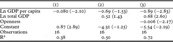
The determinants of the capital goods price data have been explored econometrically by regressing the relative price of machinery and equipment on the log of initial GDP per capita, the log of total GDP, and a measure of the degree of openness.Footnote 17 Each observation in the regression represents a particular country at the beginning of a five-year period, from 1951 to 1976.Footnote 18
Which kind of relationship should we expect between the income level and the relative price of capital goods? A major feature of the literature reviewing the structural explanations of the international comparative price level is the emphasis on the distinction between tradable and non-tradable goods. It is typically assumed that the law of one price holds for tradable but not for non-tradable goods, which are dominated by services.Footnote 19 In a world of perfectly integrated commodity markets, where all goods were tradable and transportation costs were zero, the relative price of capital goods should be identical across countries, and every country's time series of relative prices should follow the same trend. Even though machinery and equipment are tradable goods, the presence of transport costs and tariffs will cause machinery prices to diverge across countries according to international differences in productivity or skill endowments. High-income countries should exhibit lower relative prices for machinery than low-income countries.Footnote 20 The reason for this is that high-income countries have comparative advantages in the production of machinery and equipment which are more skill-intensive activities. For these reasons, we must therefore expect a negative relationship between income level and the relative price of machinery goods.
Which kind of relationship should we expect between the degree of openness and the relative price of capital goods? By specializing in their respective comparative advantages, lower-income countries will tend to buy equipment in the most advanced countries where prices are lower in relative terms. The persistence of differences in the relative price of machinery goods between countries is due to barriers that are natural to trade (such as distance, language, etc.) or to the presence of political barriers to trade. We should therefore expect a negative relationship between the relative price of machinery and the degree of openness of a country.
The regressions shown in Table 5 highlight three key relationships. First, GDP per capita is negatively related to the relative price of equipment. This result is consistent with the aforementioned literature that finds a negative relationship between income per capita levels and relative price of machinery, and justifies this pattern with the hypothesis that countries with relatively high income levels and higher productivity are generally characterized by relatively cheap capital goods. Second, for a given level of GDP per capita, the overall size of the domestic economy is positively correlated with relative equipment prices. Third, greater openness is associated with lower relative prices. Throughout the period, the degree of openness increased, so we can interpret the negative sign by suggesting that a higher degree of openness favoured the reduction in the relative price of machinery and equipment. These results corroborated one of the hypotheses of this article, which emphasizes the positive effect that international trade liberalization had on the lowering of machinery and equipment prices.
Dependent variable: the relative price of machinery, 1951–76

Source: Data of GDP, GDP per capita and openness are from Penn World Table 6.2.
Note: The dependent variable is the relative price of equipment at the beginning of the relevant period. GDP per capita, total GDP and the openness rate also pertain to the beginning of the period.
4. The investment equation and the user cost of capital
4.1. The user cost of capital
Many studies have established a robust link between the relative price of capital and economic growth. However, as Collins and Williamson (Reference Collins and Williamson2001) state, in this relationship a decisive link is generally missed. Capital goods prices always influenced growth through the investment rate. Hence it is the user cost of capital and not the relative price of capital goods that is the relevant variable in the investment model. The user cost of capital is determined by a combination of conditions not only in capital goods markets but also in financial markets. As expressed in the Hall−Jorgenson formula,Footnote 21 the user cost expression is derived under profit maximization using capital accumulation identity and the assumption of no adjustment costs:
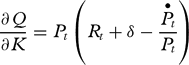
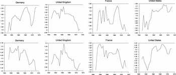
where Pt is the price of capital relative to the price of output, Rt is the real interest rate and δ is the depreciation rate. Expressed in logs, the cost of capital is the sum of two components, the relative price of capital and the non-price component. If we look within specific categories of capital goods, the two components of cost seem to have very different properties. The relative price of equipment has a very persistent downward trend in all four countries that was particularly steep from the mid 1960s until 1973, as shown in Figure 2 above. Meanwhile, the price component of structures seems to follow an upward trend throughout the entire period (see Table 1).
Those capital goods most affected by technological change, such as machinery and equipment, are more sensitive to relative price decreases.Footnote 22 Originally, the pattern of declining relative prices for equipment comes from technological innovations in equipment-producing industries. Additionally, imports of machinery from most developed countries could enhance relative price decreases in less developed countries, as has been tested in Section 3. By contrast, real interest rates, in the long run, are more closely related to the marginal productivity of capital, which tends to be a stationary variable in any general equilibrium model.
Expressed in logs, the cost of capital is the sum of two series − the relative price of capital and the non-relative-price component, which measures the required rate of return on investment. As Figure A1 in Appendix 2 shows, these two components affect the machinery and structures cost of capital series in very different ways. In the first line of Figure A1, the user cost of aggregate capital is drawn for each country; in the second line, only the user cost of equipment is shown. We can observe a distinct downward trend for the cost of equipment. Nevertheless, this downward trend is not present in the case of total investment. The downward trend in the case of machinery and equipment user cost is due to the relative price component dominating the non-price component.Footnote 23
4.2. Investment equation: econometric modelling
The objective of the econometric analysis presented in this section is to verify the factors that determined the capital stock adjustment during the Golden Age and to test the relative importance of the user cost in this process. For this purpose, we estimate the capital stock adjustment equation (equation 2) whose theoretical foundations are presented in Appendix 2. The basic regression we run can be written as

Where i t is the ratio of gross investment at time t to the gross capital stock at time t−1, y t is the ratio of GDP to the gross capital stock at time t−1; rt is our measure of the user cost of capital at time t and μj are country dummies.
Recent research on investment decisions suggests that real investment becomes more sensitive to changes in the cost of capital when relative capital prices lead the user cost. This seems to occur when the price component of cost experiences a sharp decline due to technical change or to changes in market conditions.Footnote 24 For this reason, we have followed a disaggregated approach, which models investment in separate kinds of capital goods: aggregate investment, structures investment and machinery and equipment investment.Footnote 25 The disaggregated approach will allow us to verify whether machinery and equipment investment is more sensitive to the user cost and hence to relative prices and technological change.
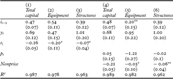
The results of the estimation using annual data are reported in Table 6 for two basic specifications: with the user cost of capital or with its two components. As the proposed regression contains the lagged dependent variable, the Ordinary Least Squares (OLS) estimate is biased and inconsistent. Therefore, in order to estimate the dynamic regression model we rely on the Instrumental Variable (IV) method. We use the previous values of the variables as instruments. In general, the instruments used appear to be valid on the basis of the Sargan test, while the results of the autocorrelation tests do not indicate major problems concerning the existence of second-order correlation that would lead to inconsistent estimates.
Dependent variable: investment over capital stock

Note: The dependent variable is the investment/capital ratio for total capital formation (columns 1 and 4), the machinery and equipment investment/machinery stock of capital (columns 2 and 5) and investment in structures/capital stock of structures (columns 3 and 6). All coefficients are significant at 5% except * that are significant at 10% and ** that are non-significant.
The results for aggregate investment (column 1) imply that investment to capital rate adjusted relatively slowly to lag values. This variable, the distributed lag function for net investment, is included in the estimation of the model to determine it. The theory itself cannot determine the rate of investment because the assumption of exogenously given output is inconsistent with perfect competition. Hence, on making the model determinate, it relies on an ad hoc adjustment mechanism. Some types of adjustment costs are introduced implicitly through the distributed lag function for investment.
The coefficient of the GDP variable is positive and significant, showing that an increase in GDP boosts the investment−capital ratio, that is to say, an increase in the product−capital ratio generates an imbalance in the quantity of capital in the economy that needs to be adjusted through an increase in investment. The GDP variable is significant and it has a positive sign in all regressions. When investment is broken down into its two components, investment in structures seems to be particularly sensitive to changes in GDP. These results fall in line with those obtained using accelerator-style models that previous studies have found best to fit the data.Footnote 26 During the Golden Age, new growth dynamics had created an economic climate with demand increases and high physical capital investment. The dynamic effects of growing markets, complementarities between physical and R&D investment, and the subsequent increase in international competition gave the investment rate more room to increase.
The user cost of capital has a significant and negative coefficient, which means that a decrease in the cost of capital will cause an increase in the desired stock of capital of the economy which will provoke an adjustment in the stock of capital through a rise in the investment−capital ratio. The elasticity of equipment investment to the user cost of capital is higher than in the case of structures investment. Part of the explanation for the cost of capital elasticity being larger in the case of equipment could be that the variance for the equipment cost of capital is dominated by persistent shocks (the embodiment of new technology that leads to a drop in machinery and equipment prices) instead of by the more volatile financial components. As shown in the previous sections of the article, the main difference between equipment and structures prices is that they moved in opposite directions. These differences are also reflected in the elasticity of investment to the components of the user cost of capital.
We break down the user cost of capital into its price (rel price) and non-price components (nonprice) and the corresponding estimations are presented in columns 4, 5 and 6. The price component is the relative price of any capital good with regard to consumption price. The non-price component refers to the real interest rate plus the depreciation rate minus the revaluation of the price of the capital goods. The coefficients of the relative price have the correct negative sign in the case of equipment investment and structures, but it is only significant in the case of equipment. However, this coefficient is higher for equipment (more than 1) than for structures (near zero). This means that machinery and equipment investment was the investment component that most responded to the evolution of relative prices during the Golden Age. This behaviour can be attributed to the permanent decline in the relative price of machinery during this period. As regards the non-price component, total capital displays a significant coefficient and, on the contrary, equipment has a non-significant coefficient in this case.
Our results are in line with recent research on investment decisions in the 1990s which suggest that real investment becomes more sensitive to changes in the user cost of capital when the relative price of capital leads the user cost. If the price component of the user cost of capital experiences a steep decline due to technical progress or to changes in market conditions, this component will be the leading force in the cost of capital.Footnote 27
5. Conclusions
The long period of high and uninterrupted growth experienced by European countries in the two decades that followed World War II has received a great deal of attention in the literature, which has highlighted a variety of interesting explanations. On the supply side, the conclusions among different authors vary in terms of the relative importance attributed to the catch-up hypothesis, the structural change hypothesis or the reconstruction effort. Demand-side explanations highlight the emergence of new institutions during the Golden Age that favoured demand stability and the expansion of international trade. Many have argued that high rates of investment played an important causal role in the Golden Age but none, until now, have highlighted the drop in the user cost as a significant contributing factor.
For this purpose we have focused our attention on one of the theoretical determinant of Hall and Jorgenson's investment equation, the user cost of capital. The user cost of capital was mainly driven by the decrease in the relative price of machinery and equipment throughout the whole period. Declines in the relative price of machinery have been interpreted in the literature about economic growth and growth accounting as a signal of the embodiment of technological change in new equipment. In this article, we do not demonstrate the embodiment of technological change, as this would require the use of other analytical tools. Instead, we have broken down aggregate investment into its two main components, machinery and structures, and have estimated the corresponding investment equations separately. This exercise reveals that equipment investment was more sensitive to the cost of capital than investment in structures and aggregate investment. This study has shown that the relative cost of machinery and equipment dropped sharply during the Golden Age and this caused investment to increase. The relative cost of structures did not experience the same decline, thus its contribution to investment growth was less. Hence the embodiment of technological change in new equipment appears as an outstanding variable in the explanation of the investment boom in machinery during the Golden Age.
In addition, the upsurge of international trade after World War II plays a significant role in the explanation of the decline in the relative price of machinery. The empirical evidence presented in this article suggests that trade liberalization contributed to the decline in the relative price of machinery in European countries in the two decades after the war. Trade liberalization increased the availability of foreign machinery that was cheaper (or better quality) and increased the share of foreign goods in domestic investment, especially in European countries. The availability of foreign machinery helped to reduce domestic machinery prices, which in turn increased the real investment rate as shown in the econometric estimation of the investment equation.
Can our hypothesis shed any light on the factors that led to the end of the Golden Age? Stagnation in relative machinery prices and the subsequent stagnation of investment rates after the first oil shock are two facts that can be drawn from the data used, particularly where European countries are concerned. However, the origin of this stagnation in prices is more difficult to determine. Bearing in mind the type of analysis carried out, nothing can be said about whether or not it was a break in technological progress that provoked this situation. But what we can prove is that during the economic crisis from the mid 1970s to 1982, trade in machinery and equipment decreased, particularly in Europe, and this led to imported equipment stagnating as a component of domestic investment. As a consequence, we can therefore conclude that machinery trade did not play the role of technology disseminator to the extent that it did during the Golden Age. Additionally, we should investigate the reasons that led to the decline in imports of capital goods; we could even dare to maintain, as many have argued, that this decline simply reflects the inevitable end of the catch-up.
Acknowledgements
A. Cubel is grateful for financial support from the Spanish Ministry of Education (SEJ2004-07402). M. T. Sanchis is grateful for financial support from the Spanish Ministry of Education (SEJ2006-08188/ECON). A preliminary version of this research was published by the Fundación de las Cajas de Ahorros (FUNCAS) as Working Paper N.276 in 2006.
Appendix 1. A new data set from 1950 at international 1985 PPPs
Our data set consists of annual series from 1950 to 1987 for real output, as well as real investment, real capital stock and the cost of capital for total capital, equipment and structures. All these series are valued at 1985 PPPs (purchasing power parities) and we had to make an effort to construct the data, as the information contained in the Penn World Tables, while widely used by other authors to analyse the relationship between the relative prices of capital and economic growth, was insufficient to cover the objectives of this article. First, the PWT only provides data from 1960 onwards and does not cover the 1950s. Second, data are not detailed enough to analyse investment in machinery and equipment. For these reasons we decided to engage the annual series of GDP, aggregate investment and its two components (machinery and structures) from 1950 until 1987, and to express them at international 1985 PPPs. The choice of 1985 as the benchmark year was in order to remain coherent with O'Mahony's (1996) internationally comparable series of capital used to estimate the Hall and Jorgenson investment equation. The data sources used are:
• GDP, aggregate investment, machinery and equipment investment, structures investment at 1985 PPPs since 1950: the 1985 PPPs from the United Nations and the Commission of the European Communities (1994) and annual data series from OECD National Accounts.
• Internationally comparable series of relative prices of capital for 1950–85: we have followed Collins and Williamson's (2001) procedure. The annual series of prices at internationally comparative levels have been constructed for each country taking as reference the 1985 PPPs of the International Comparisons Programme (ICP) of the United Nations. First, we assembled annual series of investment and consumption prices from the OECD National Accounts price deflators. Second, we used the benchmark data from the ICP for 1985 to build internationally comparable relative prices of capital goods. Third, we constructed annual series of the relative prices of capital goods and their components by backwardly discounting the annual variation rates of the implicit price indexes for investment and consumption, extracted from the OECD National Accounts.
• Capital stock: O'Mahony (Reference O'Mahony, van Ark and Crafts1996).
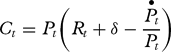
• User cost of capital: the cost of capital is measured by using the Hall−Jorgenson rental rate formula:
(A1)Where P t is the price of capital relative to the price of output, R t is the real interest rate and δ is the depreciation rate. For P t we have taken the series of relative prices described above. We have considered a constant depreciation rate, taking into account a productive life of 25 years for structures and 15 years for equipment, and a weighted average of these two rates for the aggregate. We are aware of the biases that such a choice could provoke in the results, especially if we take into account one of the main hypotheses in our work: the importance of the embodiment of technological change in machinery and equipment investment that possibly increased the depreciation rate and hence provoked changes in the investment rate. Nevertheless, taking more accurate measures of the depreciation rate into consideration goes beyond the scope of this work. To construct the real interest rate Rt we have followed Tevlin and Whelan (Reference Tevlin and Whelan2003). We subtracted expected inflation – proxied by the average inflation rate of the output deflator over the previous five years − from the nominal rate of long-run nominal interest rates. We then added a constant ‘risk premium’ that normalized this required rate of return so that its average equalled the average rate of return on physical capital, where this is measured as the ratio of nominal capital income to the nominal capital stock.
• Openness: Heston, Summers and Aten (2006); Penn World Table, vol 6.2, Center for International Comparisons of Production, Income and Prices at the University of Pennsylvania.
• Trade of capital goods: United Nations Yearbook of International Trade Statistics for the years 1953–62 and Feenstra et al. (Reference Feenstra, Lipsey, Deng, Ma and Mo2005) for the years 1962–73.
Appendix 2. Investment equation
In order to implement the relationship between investment and the relative price of capital empirically we use a traditional model of investment as a basis. Traditional models of investment start with a theory that relates the optimal frictionless capital stock, Kt*, to production technology and factor prices, in which the long-run capital stock is a function of the user cost of capital (r) and the level of demand (Y):
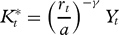
Where a is a constant and γ a parameter. If firms could adjust capital stock without incurring in costs, they would always set Kt = Kt*. In this case the investment function would simply be:

We divide by K t−1 and linearize around the steady state. However, the sluggish behaviour of capital stock suggests that there are costs associated with adjustment to desired capital stock. Traditional neo-Keynesian investment models used simple ad hoc specifications of the effects of adjustment costs, the most common being the partial adjustment approach, which assumes that firms move part of the way towards their optimal frictionless stock each period. Hence we assume the presence of adjustment costs: that is, actual capital stock will not adjust immediately to the optimal level and we have to include the lagged dependent variable. The basic regression we run can be written as

Where i t is the ratio of gross investment at time t to the gross capital stock at time t−1, y t is the ratio of GDP to the gross capital stock at time t−1; rt is our measure of the user cost of capital at time t and μj are country dummies.
User cost of capital: aggregate investment (first line) and machinery and equipment investment (second line) (1952–73, in logs)