

Introduction
The standard deviation (SD, in mathematical formulas usually represented as S or s) is one of the most popular measures of variability of quantitative variables across science disciplines, and agronomy is no exception. Most – if not all – researchers working with agronomy experiments at least have heard of it, and quite a few consider it an important measure to report when presenting results of designed experiments.
Should one indeed report treatment SDs when analyzing a designed experiment, usually with ANOVA? And what kind of information do treatment SDs convey?
We will not ponder whether SD is, in general, a good measure of variability, and we will not ponder whether, to show a variable’s variability, we should choose SD or variance or coefficient of variation (CV) or a box plot or any other measure or display. We just accept that most researchers know and use SD. Our discussion will focus on reporting group means from designed experiments, which we nearly always do when reporting ANOVA results for a designed experiment in agronomy.
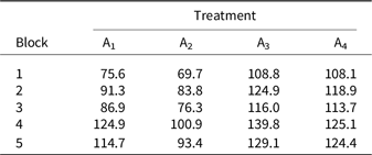
This paper thus aims to offer a recommendation on whether or not one should report groupwise SDs when reporting ANOVA results for a designed experiment; Thakur et al. (Reference Thakur, Uphoff and Antony2010), Fiorini et al. (Reference Fiorini, Boselli, Amaducci and Tabaglio2018), and Ndoli et al. (Reference Ndoli, Baudron, Sida, Schut, Van Heerwaarden and Giller2019) are recent examples of such a use of SD. To illustrate the alternative measures, we will use an artificial example of an experiment laid out in a randomized complete block design, with four treatments and five blocks (Table 1). This data set reflects a common experimental design used in agronomy research.
An artificial data set used in the paper, representing the results of an experiment in a randomized complete block design, with four treatments and five blocks

What is Standard Deviation?
The SD is a measure of variability of a variable. A formula for its sample estimate from a simple sample (i.e., for independent observations that come from the same population) is
 $${\rm{SD}} = \sqrt {{1 \over {n - 1}}{{\sum\nolimits_{i = 1}^n {({x_i} - \overline x)} }^2}},$$
where x i is the ith sample element of variable x and  $$\overline x$$ is the sample mean of x.
In designed experiments, however, observations come from simple samples only in the case of a completely randomized design. In a randomized complete block design, they do not: observations from different blocks do come from different populations (or subpopulations, depending on how we define the populations studied). Henceforth, we will call the estimator (1) the ‘raw SD’, which means it assumes the observations x i are independent. Thus, if we apply this estimator for a block design, we disregard the blocks altogether; put generally, a raw SD makes no adjustments for the design or the model.
SD quantifies the amount of variation in data: as follows from (1), SD represents the variation around the mean. A low value of SD means the data tend to be close to the mean, while a high value means the data spread over a wider range of values. We should remember that, like a mean, SD is sensitive to outliers. We are not going to discuss SD in detail; readers can find much more information in numerous statistics textbooks (Agresti and Franklin, Reference Agresti and Franklin2013; Quinn and Keough, Reference Quinn and Keough2002; Sokal and Rohlf, Reference Sokal and Rohlf1995). Suffice it to say that SD is one of the most important measures of variability, which is crucial for understanding many quantitative distributions, such as the normal distribution.
Should we report SDs for designed experiments?
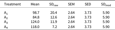
Being so important a measure of variability, SD is an inherent element of most statistical methods. Many researchers report SDs along with group means from designed experiments (as we did in the first three columns of Table 2). To consider whether reporting SDs for designed experiments is reasonable, let us first think why researchers do so.
The analysis for the data set presented in Table 1. SDraw: raw standard deviation; SEM: standard error of the mean; SDmod: model-based standard deviation

One likely reason is the ANOVA assumption of variance homogeneity. Assuming homogeneity of variance, we also assume homogeneity of treatment SDs. This assumption is important for ANOVA (Quinn and Keough, Reference Quinn and Keough2002) and should thus be checked – without exception – for each ANOVA model. Table 2 shows that treatment SDs differ (that for A4 is almost three times smaller than that for A1). Does this suggest variance heterogeneity might be a problem?
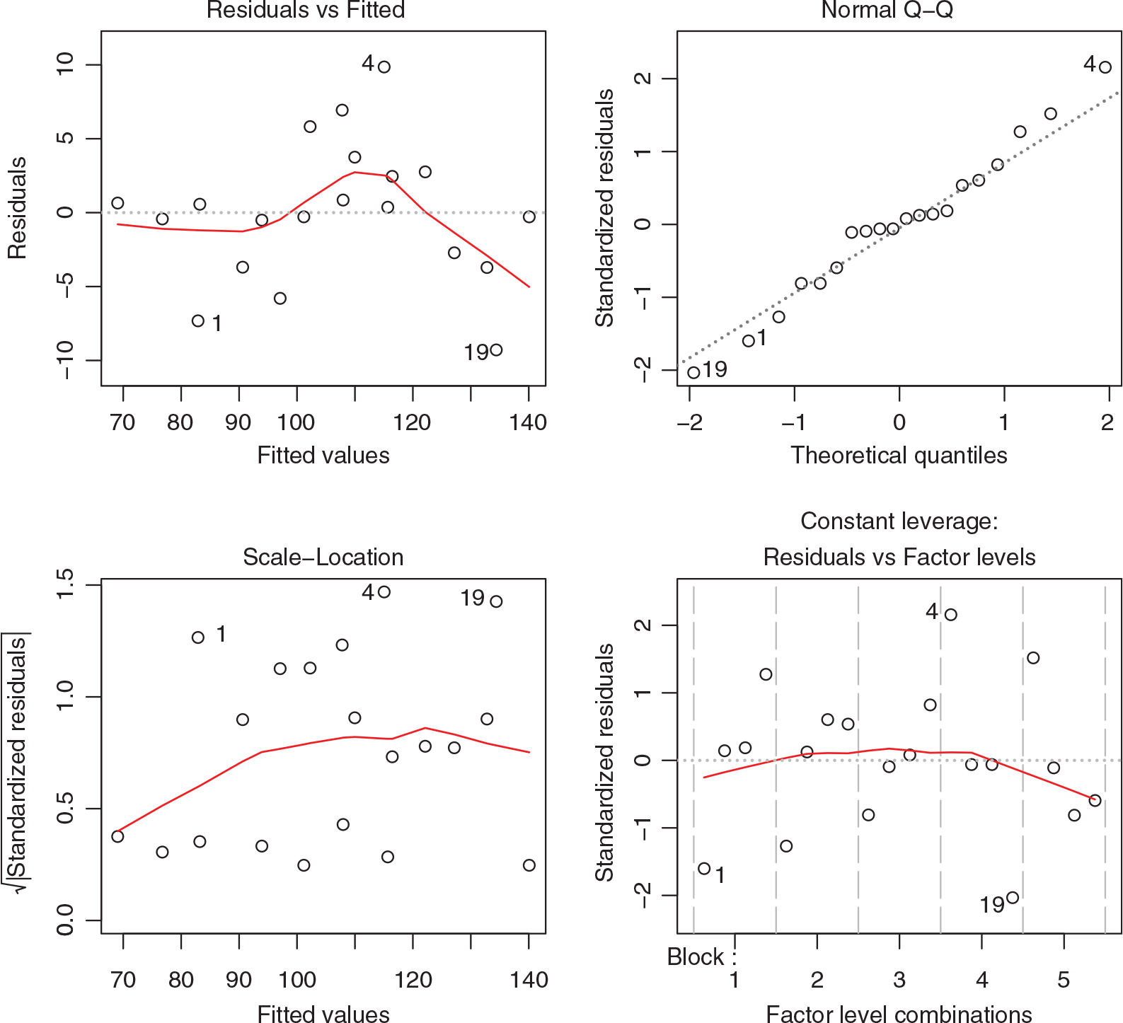
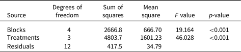
Not necessarily: as we suggested in another paper (Kozak and Piepho, Reference Kozak and Piepho2018), neither raw SDs nor statistical tests are very helpful for checking this assumption. This is especially important for block designs (so common in agronomy), in which treatment SDs are due to within-treatment variation and blocks (whose variation increases treatment SDs). Graphical methods offer better tools. Figure 1 suggests there is nothing wrong with the model fitted (Tables 2 and 3). We should not check the normality assumption in ANOVA in a groupwise fashion (Kozak and Piepho, Reference Kozak and Piepho2018). This is mainly because groupwise data have fewer degrees of freedom and, in block designs, they mix data from various blocks. Blocks are often an important source of variation, a source we would fully ignore when calculating raw SDs per treatment – because such SDs confound (mix up) both these effects; thus, we would not know whether a large SD means that the trait’s variability is great within blocks or that the between-block variability is great or both. While raw SDs mix various sources of variation, model residuals take into account all sources of variation the ANOVA model includes.
Residual graphical analysis for the ANOVA model applied to the data from Table 1. The model looks correct.


If so, should we pay attention to treatment SDs and report them along with the corresponding means? Let us ponder what would we do it for. What kind of information do raw SDs provide? How could we use them?
The primary reason for researchers to report raw SDs when presenting ANOVA results is that SD is a measure of treatment-wise variability of the data. As we discussed above, in experiments laid out in block designs such information can be misleading. Only in completely randomized designs do raw SDs have some meaning, but this meaning is of small importance, and some model-based measures (such as standard errors of the mean (SEMs) or standard errors of the difference (SEDs) carry more information.
In the context of designed experiments, however, raw SDs are appropriate only for completely randomized designs, because the only source of variation (of course, in addition to residual variation) is treatments. For instance, in agricultural research, completely randomized designs are fairly uncommon, and in field experimentation they are almost never used – most experiments follow a block design. In addition, sample sizes in agricultural experiments (and field experiments in particular) are usually so small that calculating treatment SDs based on such small samples can be risky. Many would agree that reporting only means from a designed experiment leaves us without any clue about the within-group variability, and so we should not omit SDs. This is only partly true, however, because, as discussed above, in ANOVA we assume that population SDs are the same in all treatments, and we check whether this assumption is warranted before proceeding with ANOVA. If so, it does not make sense to report treatment raw SDs following ANOVA with these assumptions checked to hold true – reporting them suggests that we would not make the above assumptions about the equality of treatment SDs.
Statistics, however, offers other possibilities than SDs. The most often used ones are SEMs or SEDs (both included in Table 2). It is crucial, however, that when we are reporting ANOVA results, SEMs should not be estimated as raw SD, divided by the square root of sample size. Instead, they should be estimated based on the fitted model. Thus, if we have, for example, a balanced experiment laid out in a randomized complete block design, means of a trait studied should have the very same SEM for all the treatments – and we need to report only this one SEM. Such SEMs are computed based on a fitted linear model and are better than those estimated ‘model free’ from raw SDs because the former use all the available degrees of freedom while the latter only uses those for the particular treatment.
One of the reasons some authors provide raw SDs is because they are easy to find. Unlike raw SDs, model-based SEMs or SEDs can be difficult to find. Indeed, not all software provides SEMs for designs more complex than completely randomized design. For instance, standard functions used for ANOVA in R (R Core Team, 2019) – lm() and aov() – do not provide SEMs, and so the users have to use the emmeans package (Lenth, Reference Lenth2019). SEDs, however, are easily accessible via the summary function applied to an lm object. Alternatively, the summary function applied to a glht object of an lm object gives an easy way to obtain SEDs for any pair of means. SAS offers various options to obtain SEMs and SEDs, like the LSMEANS statement of the MIXED, GLIMMIX, or HPMIXED procedures.
We do not mean to criticize R or SAS or any other software for not providing such measures in their standard output. Many authors need or want to provide various quantities, so it is not possible to report everything in the standard output of such functions – instead, one should use additional options or functions the software offers, in order to find those and other advanced estimates. In addition, we wish to stress that the ease of finding raw SDs is no good reason for reporting them when other measures should be reported instead. Therefore, whichever software is used, one should always try to find out how to obtain estimates one wishes to report.
Calculating SEMs and SEDs for balanced completely randomized and randomized complete block designs is straightforward:
 $${\rm{SEM}} = \sqrt {{{MSE} \over n}} {\rm{\ and\ SED}} = \sqrt {2{{MSE} \over n}} ,$$
where MSE is the mean square error for the residual term from the corresponding ANOVA model and n is the number of replications per treatment.
Thus, the SEMs from Table 1 for all means are equal to
 $${\rm{SEM}} = \sqrt {{{MSE} \over n}} = \sqrt {{{34.79} \over 5}} = 2.64,$$
and the SEDs for all pairs are equal to
 $${\rm{SED}} = \sqrt {2{{MSE} \over n}} = \sqrt {2{{34.79} \over 5}} = 3.73.$$
Note that SED is useful also in statistical testing (a topic we do not cover in this paper), because critical differences for common tests, like the t-test and Tukey’s HSD test, are directly computed from the SED. A formula for the confidence interval of the difference between the means also uses SED.
In the case of unbalanced experiments, however, we may need to report more SEMs or SEDs. If one treatment has a different number of replications than the others, then this one treatment will have a different SEM than the other ones. Also, all SEDs involving this treatment will differ from those SEDs that do not involve it. In an extreme situation, all treatments will have different numbers of replications, in which case there would be as many SEMs as there are treatments and as many SEDs as there are pairs of treatments.
But unbalanced experiments require more complex estimation for SEMs. Although in unbalanced experiments the number of different SEDs may be equal to the number of comparisons, and so reporting all SEDs may not be a feasible option – it may be a more relevant and sensible option than reporting SEMs. When there are only two different SEDs – that is, one for comparisons involving one particular treatment, and another for the remaining comparisons – reporting SEDs should not pose problems. Such a situation occurs, for example, in designs involving a control that has more replications than the other treatments, quite a common situation in agronomy experiments. When there are more than two SEDs but these do not differ too much, one can provide an average SED (the default solution in GenStat). However, when SEDs differ much, such a solution can be misleading – and then the best solution is to provide all SEDs that one considers important for the analysis one reports. Note also that SEMs and SEDs are related, but this relation depends on the design. The interested reader can find relevant information in Searle et al. (Reference Searle, Speed and Milliken1980), who cover the complex topic of estimation of SEMs and SEDs in unbalanced experiments.
The point is that in ANOVA, treatment SEMs represent the precision of the estimators of the means. To interpret treatment means themselves, we would indeed use the means along with their SEMs. But this is not what agricultural researchers strive for, at least not usually, because such interpretation does not enable treatment-to-treatment comparison. In agriculture, we usually prefer to compare means of two treatments – and this is exactly what SED is designed for.
Model-based SDs
Kozak et al. (Reference Kozak, Bocianowski and Rybiński2013), discussing agricultural experimentation, suggested that, for designed experiments, a model-based CV is more informative than a raw CV. It is estimated as the square root of the MSE divided by the mean. The reasons they provided were similar to those above: a raw CV (i.e., estimated based on raw data of the whole data set) ignores various sources of variation, so it does not say much about the within-group variability. Instead, it mixes the between-group variability with the within-group variability, adding also variability that is due to blocks.
Following this reasoning, should we be adjusting raw SDs for the analyzed model and reporting such adjusted – or model-based – SDs? The only software we are aware of that directly uses the term ‘pooled SDs’ is MINITAB. Many others do it too but do not use this name. For instance, R calls this measure ‘residual standard error’ (an unfortunate term because it confuses the terms standard error and standard deviation) and SAS calls it ‘root MSE’. With so different terms used, the readers can be confused what these measures – or rather this one measure with so many different names – show. The online manual for the GLM procedure of SAS says, ‘Root MSE estimates the standard deviation of the dependent variable (or equivalently, the error term) and equals the square root of the Mean Square for Error’ (this explanation also mixes two terms: SD of the dependent variable and SD of the error term) (SAS Institute, 2009).
In our example, we have all the information we need to calculate pooled (model-based) SDs – because it is equal to the square root of the MSE. From Table 3, we know the MSE is 34.79, so its square root is 5.90 – and this is the value of the model-based SD (Table 2). Note again that since we assume all treatment SDs are the same, this value is the same for all treatments.
Using Equation (2), we observe that for balanced data the following relations hold:
 $${\rm{SEM}} = \sqrt {{{MSE} \over n}} = {{{\rm{S}}{{\rm{D}}_{\,\bmod \,}}} \over {\sqrt n }}\,{\rm{and}}\,{\rm{SED}} = \sqrt {2{{MSE} \over n}} = \sqrt 2 {\mkern 1mu} \,{\rm{SEM}} = \sqrt 2 {{{\rm{S}}{{\rm{D}}_{\,\bmod \,}}} \over {\sqrt n }},$$
where SDmod is the model-based (pooled) SD.
Model-based SDs are free of the above-discussed drawbacks of raw SDs. But does this mean we should prefer them over SEMs or SEDs? In our opinion, the answer is ‘no’. Statistical procedures for designed experiments provide various possibilities of inference, and these possibilities are tailored to the design and the inference needs. Model-based SDs, on the other hand, are not that popular and not that easy to understand for non-statisticians. What’s more, reporting them is not enough – we should still give SEMs or SEDs. This is because, when planning a comparative experiment, we intend to compare treatment means. Thus, focusing on comparing means, we should report what is needed to do so – and SED, not adjusted SD, aims to help us understand, interpret, and compare treatment means. A pooled (or model-based) SD represents a trait’s variation that is due to individual-to-individual variation, all other sources of variation (such as treatments or blocks) being accounted for. In the case of designed experiment, such information is seldom relevant – which is why we do not consider it important enough to report, and for certain not important enough to use it instead of SEMs or SEDs.
A common related misunderstanding we wish to clarify is to assume that one can compare several means using their confidence intervals. It is often falsely believed that if confidence intervals of two means overlap, their difference is nonsignificant. For balanced data, this would be the case if SEDs were equal to 2 SEM, but – as follows from Equation (3) – this is not the case, since  $${\rm{SED}} = \sqrt 2 $$. For unbalanced or correlated data, this rule of thumb does not work, either. Thus, to compare two means, one should explicitly estimate a confidence interval for the difference.
Conclusion
What to report from a statistical analysis does matter. The results we decide to present should be important for understanding the data, the phenomena studied, and the statistical analysis we conducted. This list should not include measures that can be confusing or unclear or even misleading for the reader.
On the one hand, most readers of agricultural and biological journals are familiar with the concept of SD, and importantly, most of them know that this measure represents variation of a variable. So, could SD be confusing? Yes – and in fact, reporting SD can be misleading because so many readers will not be aware of the above-discussed problems related to its use for designed experiments. Design-based SDs are so uncommon that most readers may have problems understanding them.
Discussing ANOVA applied to analyze soil science experiments, Webster (Reference Webster2001) pointed out that SD ‘measures the dispersion in our observations; it does not immediately tell us how reliable is our estimate of μ’ (μ being a population mean a sample mean aims to estimate). So, if we indeed want to provide some estimate of this dispersion, we can use model-based (but not raw!) SDs in addition to standard errors – but doing so, we should help the reader understand why we present model-based SDs and what they mean in the context of the experiment analyzed. Our last recommendation about this measure is as follows: double-check the reason for wanting to provide this measure because in most agronomy scenarios this measure will not tell the story the reader expects to hear.
Situation gets even more complicated for more complex designs. We have shown that raw SDs can be misleading in such a simple and common design as randomized complete block design. This is because in this case variation in a trait studied is a mixture of variation having three sources:
(i) the variation due to treatment applied;
(ii) the variation due to blocks; and
(iii) the intrinsic variation among individuals (the so-called residual variation), which itself can have two sources: environmental and genotypic.
Raw SDs mix up the last two sources. When an experimental design is more complex – as is the case with split-plot designs, repeated measure designs, and repeated experiments, where random effects need to be fitted – such raw SDs would mix up even more sources of variation, since such an approach takes into account only the first source of variation – due to treatments – and combines all the other ones. Use of such raw SDs is of no value and can do more harm than good, and thus should never lie in the interest of a person interpreting the results of a designed experiment.
Our whole discussion deals with ANOVA-like scenarios. Regression analysis, however, is quite similar, both ANOVA and regression being particular versions of the general linear model, ANOVA dealing with qualitative factors and regression with quantitative ones. Just as we can report SEDs for means of qualitative factors in ANOVA, we can report SEDs for regression coefficients in regression analysis. This is very rarely done, however. Piepho et al. (Reference Piepho, Williams and Fleck2006) offer an example of such a comparison of regression coefficients using SED. It is stressed here that all we have discussed in terms of ANOVA equally applies for the regression analysis for a designed experiment.
In our opinion, thus, treatment means from a designed experiment should not be accompanied by the corresponding SDs, whether raw or model-based. Except for the completely randomized design, the former do not even represent within-group variability. The latter would be too difficult to interpret for many readers, but also would be insufficient – SEMs or, even better, SEDs would need to be presented.
Financial support
None.