1. Introduction
Collision, merger and breakup of liquid drops are observed in nature and numerous engineering applications. For example, the development of free-surface instabilities that results in liquid fragmentation in fuel atomization systems is one of the critical processes affecting proper reaction rate of combustion and functionality of various fluid devices. The design of atomizers and spray nozzles may intensively rely on empirical estimations or on the knowledge of breaking mechanisms based on observations and physical reasoning. The features of the phase boundary span from centimetres to micrometres and evolve in the time scale of milliseconds. For example, droplets produced during liquid jet impingement in an air-breathing or rocket engine result in the Weber number (
 $\mathit{We}={\it\rho}U^{2}l/{\it\sigma}$
, where
 ${\it\rho}$
,
 ${\it\sigma}$
,
 $U$
and
 $l$
are the liquid density, surface tension coefficient, characteristic velocity and length scale, respectively) varying from order of
 $O(1)$
to
 $O(10^{5})$
(Anderson, Ryan & Santoro Reference Anderson, Ryan, Santoro, Yang and Anderson1995). While under the full power condition, gas turbine combustion dynamics can be reasonably handled by the gaseous phase model, Correa & Shyy (Reference Correa and Shyy1987) and Shyy, Correa & Braaten (Reference Shyy, Correa and Braaten1988) for conditions related to start-up, high altitude, relight and other transient processes, multiphase dynamics need to be included. Various issues related to drop dynamics and combustion were reviewed by Faeth (Reference Faeth1983) and Law (Reference Law2010). The droplet collision regimes were systematically studied by Qian & Law (Reference Qian and Law1997) in the range of Weber number below 100. Later, many numerical works were conducted in order to replicate droplet collisions at the same conditions of Qian and Law. Studies using volume-of-fluid (VOF) (Gotaas et al.
Reference Gotaas, Havelka, Jakobsen, Svendsen, Hase, Roth and Weigand2007), level-set (Pan & Suga Reference Pan and Suga2005) and front-tracking methods (Singh & Shyy Reference Singh and Shyy2007; Pan, Law & Zhou Reference Pan, Law and Zhou2008) can successfully resolve the essential features of interfaces and the collision dynamics, which have been shown in the experimental works in the low- and modest-Weber-number regime. Pan, Chou & Tseng (Reference Pan, Chou and Tseng2009) presented experimental measurements of higher-speed, binary head-on collision at Weber numbers ranging from 200 to 5000. The experiments show interface expansion, fingering, retreating and prompt splattering as the Weber number increases. The collision outcome is similar to the droplet splashing on solid plates without the surface roughness and wetting effect of the solid phases. Due to the high speed and small length scale, the experimental images provide limited information for the understanding of interface breakup mechanisms. The colliding droplets experience coalescence, violent deformation and then breakup. The size of shattered satellite droplets is reduced dramatically with the increasing Weber number. To date, three-dimensional numerical solution for high-Weber-number collision is absent because numerous significant issues related to computational algorithm, modelling fidelity, as well as experimental validation need to be resolved. In this paper, we report a parallel, adaptive Eulerian–Lagrangian interface-tracking framework for solving the high-Weber-number binary droplet collision that corresponds to the experimental efforts reported by Pan et al. (Reference Pan, Chou and Tseng2009). Two equal-size droplets are manipulated to collide head-to-head at the same impinging speed. Based on combined computational and experimental efforts, we have resolved for the first time the free-surface instabilities of the colliding droplets at high Weber number. We also provide a detailed account of interfacial characteristics related to drop collision and merger, free-surface instabilities and the breakup dynamics. A number of cases of different Weber number are considered to explore the interplay between inertia, viscosity, pressure and surface tension. Highly varied development corresponding to different control parameters is documented.
The present solver is based on the Eulerian–Lagrangian interface-tracking method developed by Singh & Shyy (Reference Singh and Shyy2007), Uzgoren et al. (Reference Uzgoren, Singh, Sim and Shyy2007) and Sim & Shyy (Reference Sim and Shyy2012). We further incorporate this Eulerian–Lagrangian interface-tracking method in a distributed-computation framework with a parallel adaptive mesh refinement (AMR) technique. We address parallelisms employed for Lagrangian and Eulerian domain and a cell-based unstructured AMR.
The Eulerian–Lagrangian interface-tracking method adopted in this study is based on the immersed boundary method. A set of connected Lagrangian markers represent moving phase boundaries. The field equations are solved on an Eulerian Cartesian grid, while Lagrangian boundaries propagate according to the velocity field of the Eulerian grid. Interfacial effects such as surface tension force are calculated explicitly in the Lagrangian domain, and then projected to the Eulerian frame. Therefore, the Eulerian–Lagrangian interface-tracking method stores variables on Eulerian and Lagrangian frames with different data structures. Variables on the Lagrangian interfaces and Eulerian grid are coupled by a cross-domain interpolation. The size and frequency of information exchanged between the Lagrangian markers and the Eulerian grid depend on the modelling formulation of fluid boundaries. Here, the continuous interface method represents the fluid boundaries as smoothing transition of fluid properties at the boundaries Peskin (Reference Peskin2002). In addition, the Lagrangian interface requires a remeshing treatment in order to maintain the quality of the triangular surface mesh. Moreover, direct advection of interfaces does not change the interface topology. The breakup and merging of interfaces require special treatment on the connectivity of Lagrangian markers.
Bo et al. (Reference Bo, Liu, Glimm and Li2011) presented a front-tracking technique with a local grid-based method to treat topological changes, but generally, complex interface deformation remains challenging for the front-tracking family. In summary, the present Eulerian–Lagrangian method, as one of the front-tracking methods, has more algorithm complexities than Eulerian methods such as VOF and level-set methods in three aspects: cross-domain data interpolation, Lagrangian remeshing and topology change algorithm. However, the explicit representation of interfaces can provide desirable accuracy of geometries, such as curvature computation, which is one of its more difficult features.
While the current Eulerian–Lagrangian interface-tracking method is effective for interfacial computation, the method incurs significant challenges for a parallel implementation. There are two features to consider from the perspective of parallelization. First, the Eulerian–Lagrangian method is a dual-domain technique. The Lagrangian data is stored in dynamic arrays on a triangular surface mesh, as opposed to flow data on an Eulerian frame. Partition strategies must consider the distribution of workload on both domains. Second, data on an Eulerian grid cell and a Lagrangian marker are highly coupled in a computational time step. Strong data dependency in time between the Eulerian and Lagrangian domains imposes restrictions on the choice of parallelisms for scalability.
Eulerian methods such as the VOF use a scalar, material function to reconstruct and locate interfaces. Since the data structure of Eulerian methods is similar to traditional single-phase flow solvers, the parallel implementation of Eulerian methods is straightforward and usually accomplished by spatial domain decomposition (Sussman Reference Sussman2005; Ongaro et al. Reference Ongaro, Cavazzoni, Erbacci, Neri and Salvetti2007; Agbaglah et al. Reference Agbaglah, Delaux, Fuster, Hoepffner, Josserand, Popinet, Ray, Scardovelli and Zaleski2011). In contrast, there are only a few studies on parallel solvers based on an Eulerian–Lagrangian framework. Most of them focus on problems with Lagrangian particles but not for arbitrary moving boundaries, and use simple, static domain decomposition strategies. Capecelatro & Desjardins (Reference Capecelatro and Desjardins2013) presented a particle-laden flow solver for the Eulerian–Lagrangian framework. The Eulerian mesh is partitioned statically, and particles are decomposed according to their location with respective Eulerian subdomain.
Darmana, Deen & Kuipers (Reference Darmana, Deen and Kuipers2006) presented a mirror domain parallelism for an Eulerian–Lagrange model to simulate swarming bubbles columns. The Eulerian domain is uniformly partitioned along the
 $z$
-axis, and each processor holds complete Lagrangian data and conducts computation on a Lagrangian particles subset. Herrmann (Reference Herrmann2010) used the Eulerian method to capture interfaces and described the under-resolved liquid volume with Lagrangian particles. For these works reviewed, favourable performance of an Eulerian–Lagrangian-type solver was shown, which may be due to the Lagrangian data being loosely coupled with the Eulerian data, and the Lagrangian objects being individual particles (no connectivity) and uniformly distributed in the Eulerian domain. However, for many practical problems, the Lagrangian objects frequently interact with the Eulerian grid and their spatial distribution is non-uniform in the Eulerian domain.
Nkonga & Charrier (Reference Nkonga and Charrier2002) reported a parcel method for a dispersed spray in a turbulent flow of piston engines. The Lagrangian parcels are used to describe dispersed spray particles that move on a two-dimensional Eulerian unstructured mesh. Nkonga and Charrier discussed the load imbalance due to the non-uniform distribution of parcels in a domain; the result shows that the parallel efficiency is problem dependent. Pan & Yin (Reference Pan and Yin2012) evaluated the computing strategies of a two-dimensional front-tracking method on Message Passing Interface (MPI), Open Multi-Processing (OpenMP) and hybrid of MPI–OpenMP platforms. They suggested that an algorithm should consider hardware specifications and problem scale in order to achieve favourable performance. In summary, the challenges of the Eulerian–Lagrangian methods in terms of parallelization are load balanced for both Eulerian and Lagrangian domains and communication strategies. In the present Eulerian–Lagrangian interface-tracking method, a load-balanced parallelism for both Eulerian and Lagrangian computations may be possible only with a compromise in communication overhead. The parallelisms that are adopted determine the frequency and data size of cross-processor communication. Minimizing communication overhead may be achievable only by using a parallelism having an imbalanced computation load on one of the two domains. We discuss possible parallelisms for the Eulerian–Lagrangian method in the following section, and use spatial domain decomposition for the Lagrangian domain to give advantage to the data locality.
The present paper is organized as follows. First, we briefly introduce the numerical algorithm of the three-dimensional Eulerian–Lagrangian method. The interactions between the Eulerian and Lagrangian domains during computation are discussed to highlight the design consideration and then parallelisms are proposed. Parallel implementation for cell-based unstructured AMR is outlined. We analyse parallel performance, and then validate our implementation. We then conduct droplet collision simulations in the high-Weber-number regime to demonstrate the effectiveness of current approach for capturing the multiscale free-surface flow. The interfacial dynamics and associated free-surface instabilities on the edge of the merged droplet are discussed in detail.
2. The Eulerian–Lagrangian interface-tracking method
2.1. Governing equations
We solve the Navier–Stokes equations for incompressible Newtonian fluids on Eulerian Cartesian grid, as given in
 $$\begin{eqnarray}\displaystyle & \displaystyle \frac{\partial {\it\rho}}{\partial t}+\boldsymbol{{\rm\nabla}}\boldsymbol{\cdot }({\it\rho}\boldsymbol{u})=0 & \displaystyle\end{eqnarray}$$
 $$\begin{eqnarray}\displaystyle & \displaystyle \frac{\partial ({\it\rho}\boldsymbol{u})}{\partial t}+\boldsymbol{{\rm\nabla}}\boldsymbol{\cdot }({\it\rho}\boldsymbol{uu})=-\boldsymbol{{\rm\nabla}}p+\boldsymbol{{\rm\nabla}}\boldsymbol{\cdot }{\it\mu}(\boldsymbol{{\rm\nabla}}\boldsymbol{u}+{\rm\nabla}^{\text{T}}\boldsymbol{u})+\boldsymbol{f}. & \displaystyle\end{eqnarray}$$
 $\boldsymbol{u}$
is the velocity vector on the Eulerian domain, and
 ${\it\rho},{\it\mu}$
and
 $p$
are the density, viscosity and pressure, respectively. The interfacial dynamics is modelled source terms at the right-hand side of the momentum equation. In this study, the momentum force vector,
 $\boldsymbol{f}$
, accounting for the surface tension force of fluid interfaces is described in the next paragraph. Dimensionless parameters considered are Reynolds number,
 $\mathit{Re}=({\it\rho}_{l}UD_{0})/{\it\mu}_{l}$
, and Weber number,
 $\mathit{We}=({\it\rho}_{l}UD_{0})/{\it\sigma}$
, based on relative impinging speed
 $U$
, initial droplet diameter
 $D_{0}$
, liquid density
 ${\it\rho}_{l}$
and viscosity
 ${\it\mu}_{l}$
. We solve (2.1) and (2.2) by a finite-volume projection method on a staggered grid. The velocity field is computed first using the pressure based on the previous time step, then corrected by an updated pressure field via a Poisson equation constrained by the divergence-free velocity field, satisfying the mass conservation equation. The convection term is discretized by the third-order essentially non-oscillatory (ENO) scheme in space and second-order Runge–Kutta integration in time. The viscous term is obtained by the central difference discretization in space and Crank–Nicholson integration in time. The pressure distribution is obtained by enforcing a divergence-free velocity field via a predictor–corrector type of projection method. The essential information related to the Navier–Stokes solver can be found in Singh & Shyy (Reference Singh and Shyy2007, § 4.2, especially equations (8)–(12)) and Uzgoren, Sim & Shyy (Reference Uzgoren, Sim and Shyy2009, § 2, especially equations (2.4)–(2.7)). It is noted that using a finite-volume approach, linear interpolation facilitates the flux estimation between fine/coarse cells. The cell-centred variables such as pressure and density are interpolated to a cell face by piecewise linear interpolation on coarse–fine grid boundary, taking into account the cell size on either side of the face. The coefficient matrix is not symmetric due to spatially varying viscosity associated with the multifluid/multiphase interfaces. To attain desirable computational performance with parallel scalability, we have adopted the well-established Portable, Extensible Toolkit for Scientific Computation (PETSc) (Balay et al.
Reference Balay, Brown, Buschelman, Eijkhout, Gropp, Kaushik, Knepley, McInnes, Smith and Zhang2012) library, with preconditioners provided by hypre (Falgout & Yang Reference Falgout, Yang, Sloot, Tan, Dongarra and Hoekstra2002) to solve this large, sparse liner system of equation.
2.2. Interface tracking and modelling
At the vicinity of an interface, we use an indicator function
 $I(\boldsymbol{x})$
of an Eulerian point at coordinate
 $\boldsymbol{x}$
to represent fluid material variation on Eulerian domain. The indicator function is a discrete form of the Heaviside step function:
 $$\begin{eqnarray}\displaystyle I(\boldsymbol{x})=H\left(r=\boldsymbol{n}\boldsymbol{\cdot }\left(\boldsymbol{x}-\boldsymbol{X}\right)/{\rm\Delta}x\right)=\int _{-\infty }^{r}{\it\delta}_{h}(h)\text{d}h. & & \displaystyle\end{eqnarray}$$
From an Eulerian point at
 $\boldsymbol{x}$
, we search the nearest Lagrangian element with respect to coordinate
 $\boldsymbol{x}$
to determine the distance ‘
 $r$
’ and to compute the indicator function. Here
 $r$
is the distance between an Eulerian coordinate
 $\boldsymbol{x}$
and a Lagrangian marker at Lagrangian coordinate
 $\boldsymbol{X}$
normalized by the grid size
 ${\rm\Delta}x$
. In this paper, an uppercase letter denotes a variable in the moving frame while the lowercase letter marks its counterpart in the fixed frame. The indicator function is obtained by integrating the one-dimensional form of approximate Dirac delta function
 ${\it\delta}_{h}$
from liquid to gas phase, given by (2.4). The approximate Dirac delta function is based on the formulation of Peskin (Reference Peskin2002). It is calculated over a finite space, from the centre of interested point to two Eulerian cell widths
 $2{\rm\Delta}x$
in radius. This
 $2{\rm\Delta}x$
is a cut-off length of the Eulerian–Lagrangian coupling. To implement the mathematical expression in numerical terms, the choice of the radius of the delta function affects the smoothness of the flowfield around the interface as well as the computational stiffness. In many computations performed by the authors and others, the present cut-off length offers an appropriate balance. To capture the desirable flow details while addressing the smoothing operation, the present AMR technique enhances the resolution at a cell-by-cell level.
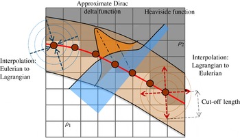
Figure 1 illustrates the approximate Dirac delta function, Heaviside function and material variation across a Lagrangian interfaces on a two-dimensional domain:
 $$\begin{eqnarray}\displaystyle {\it\delta}_{k}=\left\{\begin{array}{@{}ll@{}}\displaystyle {\textstyle \frac{1}{8}}\left(5-2\left|r\right|-\sqrt{-7+12\left|r\right|-4\left|r\right|^{2}}\right)\quad & 1\leqslant \left|r\right|\leqslant 2,\\ \displaystyle {\textstyle \frac{1}{8}}\left(3-2\left|r\right|+\sqrt{1+4\left|r\right|-4\left|r\right|^{2}}\right)\quad & 0\leqslant \left|r\right|\leqslant 1,\\ 0\quad & \left|r\right|>2.\end{array}\right. & & \displaystyle\end{eqnarray}$$
Variation of an indicator function (Heaviside function) and approximate Dirac delta function around the Lagrangian interface on a two-dimensional Eulerian domain. The coupling range of an Eulerian cell to Lagrangian marker is
 $2{\rm\Delta}x$
, the cut-off length of the approximate Dirac delta function.

The indicator function at the interface is 0.5, and varies smoothly from 0 to 1 across the interface. This indicator function locates discontinuous material properties into a continuous form. With the continuous variation of material properties across the interfaces, we solve a single set of Navier–Stokes equation to describe all fluid phases on the Eulerian domain. The continuous fluid properties are computed based on the Heaviside function
 $$\begin{eqnarray}{\it\varphi}={\it\varphi}_{2}+\left({\it\varphi}_{1}-{\it\varphi}_{2}\right)I.\end{eqnarray}$$
Here,
 ${\it\varphi}$
can be a material property such as density, viscosity and conductivity.
As discussed in Singh & Shyy (Reference Singh and Shyy2007, § 3.2), the instances of interface merger or breakup are detected using two probes in opposite directions along the local normal vector on markers. The length of each probe is set to one and a half times the background cell size and the indicator function value on these probes are bilinearly interpolated from the grid. The reconstruction is performed if both probes from a marker have indicator function value greater or less than half, representing a situation where the immersed boundary formulation does not ‘see’ an interface (when approximated by
 $\text{indicator}=0.5$
) between the two probes. In the case of multiple interfaces, the reconstruction is performed only for those requesting it while leaving others untouched.
The Lagrangian interfaces are a set of triangular elements formed by a set of markers with connectivity. The coordinate of a marker, denoted by
 $\boldsymbol{X}$
in Lagrangian frame is updated based on the marker velocity
 $\boldsymbol{U}(\boldsymbol{X})$
, given by the equation of motion as
 $$\begin{eqnarray}\displaystyle \frac{\partial \boldsymbol{X}}{\partial t}=\boldsymbol{U}(\boldsymbol{X}). & & \displaystyle\end{eqnarray}$$
The velocity of a Lagrangian marker
 $\boldsymbol{U}(\boldsymbol{X})$
is a projection from the resolved velocity field on the Eulerian domain
 ${\it\Omega}$
to the Lagrangian domain
 $\mathscr{L}$
by
 $$\begin{eqnarray}\displaystyle \boldsymbol{U}(\boldsymbol{X})=\left.\int _{V}\boldsymbol{u}(\boldsymbol{x}){\it\delta}_{h}(\boldsymbol{x}-\boldsymbol{X})\,\text{d}V\right/\!\!\int _{V}{\it\delta}_{h}(\boldsymbol{x}-\boldsymbol{X})\,\text{d}V,\quad V\in {\it\Omega},\quad V=\{\boldsymbol{x}\mid \left|\boldsymbol{x}-\boldsymbol{X}\right|\leqslant 2{\rm\Delta}x\}. & & \displaystyle \nonumber\\ \displaystyle & & \displaystyle\end{eqnarray}$$
Here
 $V$
is the vertex of the Eulerian Cartesian grid. By using the approximate Dirac delta function, the Euler-to-Lagrange interpolation of a Lagrangian marker only requires information of Eulerian vertexes that are in the radius of the cut-off length
 $2{\rm\Delta}x$
.
A Lagrangian marker diffusively projects the momentum force term to a regional Eulerian space, as illustrated in figure 1. At the vicinities of the Lagrangian interfaces, the surface tension force
 $\boldsymbol{F}(\boldsymbol{X})$
on a Lagrangian marker
 ${\it\Gamma}(\boldsymbol{X})$
is converted to Eulerian force
 $\boldsymbol{f}(\boldsymbol{x})$
on the Eulerian coordinate
 $\boldsymbol{x}$
. Similar to the Euler-to-Lagrange interpolation of (2.7), an Eulerian point only considers Lagrangian markers
 ${\it\Gamma}(\boldsymbol{X})$
in the cut-off length for interpolation weighting as given in
 $$\begin{eqnarray}\displaystyle \boldsymbol{f}(\boldsymbol{x})=\left.\int _{{\it\Gamma}}\boldsymbol{F}(\boldsymbol{X}){\it\delta}_{h}\left(\boldsymbol{X}-\boldsymbol{x}\right)\text{d}{\it\Gamma}\!\right/\!\!\int _{{\it\Gamma}}{\it\delta}_{h}\left(\boldsymbol{X}-\boldsymbol{x}\right)\text{d}{\it\Gamma},\quad \!{\it\Gamma}\in \mathscr{L},\ {\it\Gamma}=\{\boldsymbol{X}|\left|\boldsymbol{x}-\boldsymbol{X}\right|\leqslant 2{\rm\Delta}x\}. & & \displaystyle \nonumber\\ \displaystyle & & \displaystyle\end{eqnarray}$$
We compute the surface tension force
 ${\it\delta}\boldsymbol{F}(\boldsymbol{X})={\it\sigma}{\bf\kappa}{\it\delta}A$
, where
 ${\it\delta}A$
is the surface area and
 ${\bf\kappa}$
is the local curvature of a discrete Lagrangian element, by a line integral form of
 $$\begin{eqnarray}\displaystyle {\it\delta}\boldsymbol{F}={\it\sigma}{\bf\kappa}{\it\delta}A={\it\sigma}(\boldsymbol{n}\times \boldsymbol{{\rm\nabla}})\times \boldsymbol{n}{\it\delta}A=\mathop{\sum }\limits_{i=1}^{3}{\it\sigma}(\boldsymbol{t}_{i}\times \boldsymbol{n}){\it\delta}S. & & \displaystyle\end{eqnarray}$$
based on its normal and tangent vectors. The summation of cross-product of three tangent vector
 $\boldsymbol{t}_{\boldsymbol{i}}$
along the triangle edge
 $S$
and outward unit normal
 $\boldsymbol{n}$
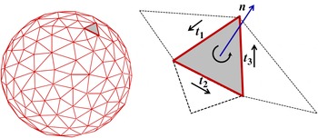
produces a local curvature of this Lagrangian element, as shown in figure 2. By integrating surface tension force from all Lagrangian elements of a close surface, the net force is zero. Direct computation of the curvature using interpolation-based methods is numerically sensitive and often requires some form of data smoothing, and does not enforce surface tension conservation on a closed surface.
Curvature computation of a discrete Lagrangian element.

Details of the numerical computation for surface tension can be found in Singh & Shyy (Reference Singh and Shyy2007), Uzgoren et al. (Reference Uzgoren, Sim and Shyy2009), Kuan, Sim & Shyy (Reference Kuan, Sim and Shyy2012) and Sim & Shyy (Reference Sim and Shyy2012). The numerical error due to the computation of interface curvature can result in spurious velocities around the interface. Such errors can dominate the flow of a long-time simulation. The accuracy of the current implementation was discussed by Singh & Shyy (Reference Singh and Shyy2007) for a static bubble problem. The magnitude of spurious velocity evaluated in a dimensionless form as the capillary number,
 $\mathit{Ca}={\it\mu}U/{\it\sigma}$
, is of the order of
 $10^{-4}$
and insensitive to the Laplace number (
 $\mathit{La}={\it\sigma}{\it\rho}l/{\it\mu}$
, where
 $l$
is the length scale) up to
 $10^{5}$
.
3. Parallel implementation
3.1. Computation-to-communication ratio
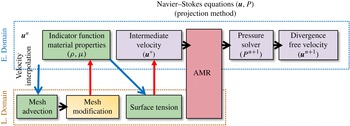
Figure 3 describes the task procedure of the Eulerian–Lagrangian interface tracking method in a computational time step. We illustrate the task procedures according to the type of computation in order to show the frame of a computation and data dependency. There are four categories of the procedural tasks: Eulerian task, Eulerian–Lagrangian task, Lagrangian task and AMR. The Eulerian tasks refer to the computation on the Eulerian frame, such as the field-equation solver. In a single time step, a serial computation usually spends approximately 60 % of wall-clock time on the field-equation solver. Therefore, the load balance on the Eulerian tasks is a priority. In addition, there are four times of cross-domain communication through the Dirac delta function for Eulerian–Lagrangian coupling. As a result, data locality is the primary factor affecting the parallel performance. This is non-trivial to achieve because the size and location of the Lagrangian mesh varies in time and space.
The solving procedure of the Eulerian–Lagrangian method.

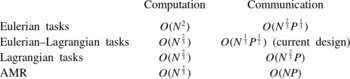
The computation-to-communication ratio primarily determines the parallel performance of all of the tasks. Table 1 summarizes computation and communication scaling with respect to a sufficiently large Eulerian grid with
 $N$
grid points and the number of processor
 $P$
used in the computation.
Scaling of computation and communication cost of the parallel, adaptive Eulerian–Lagrangian interface tracking method for a sufficiently large problem with
 $N$
Eulerian grid points and total
 $P$
processors involving in the computation.

Here, we assume that the Eulerian grid forms a cube-like domain and there is a set of Lagrangian mesh in the size of
 $c\cdot N^{\frac{2}{3}}$
, where
 $c$
is a finite positive constant and much smaller than
 $N^{\frac{1}{3}}$
. We ideally assume an averaged Eulerian grid size per processor is
 $N/P$
and the size of the partition boundary is
 $(N/P)^{\frac{2}{3}}$
. In the case of an evenly distributed Lagrangian mesh in the Eulerian domain, the averaged Lagrangian marker per processor is of the order of
 $O(N^{\frac{2}{3}}/P)$
and the size of Lagrangian boundaries per processor is
 $O(N^{\frac{1}{3}}/P^{\frac{1}{2}})$
. The leading cost of the Eulerian task is on solving the linear sparse matrix of the pressure Poisson equation by Krylov subspace methods, which is of the order of
 $O(N^{2})$
. Communication cost of the Eulerian task scales with the data size of the partition boundaries, which is order of
 $O(N^{\frac{2}{3}}P^{\frac{1}{3}})$
. The computation of the Lagrangian tasks scales with the Lagrangian surface area, as of the order of
 $O(N^{\frac{2}{3}})$
, while the communication cost is proportional to
 $O(N^{\frac{2}{3}}P)$
due to usage of all-to-all communication for the synchronization of surface mesh connectivity. A geometry-based AMR has computation cost of the order of
 $O(N^{\frac{2}{3}})$
. For synchronizing the global Eulerian graph connectivity, the data needed for exchange of AMR is of the order of
 $O(\mathit{NP})$
. Tasks such as surface tension calculation involving the Eulerian–Lagrangian coupling have computation cost of
 $O(N^{\frac{2}{3}})$
. The communication cost of the Eulerian–Lagrangian task is of the order of
 $O(N^{\frac{1}{3}}P^{\frac{1}{2}})$
using the present approach of Lagrangian domain decomposition. We explain the present domain decomposition in the next section. This communication cost can be much higher than current design by adopting a load-balanced decomposition without considering the data locality of Lagrangian markers.
3.2. Parallelism for Eulerian and Lagrangian domain
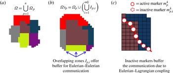
We decompose the Eulerian domain by the graph-partitioning library ParMETIS (for its multiobjective optimization on data redistribution cost, load balance, and number of edge-cut together). We suppose that an Eulerian domain
 ${\it\Omega}$
is decomposed into
 $n$
non-overlapping partitions,
 ${\it\Omega}_{p},{\it\Omega}=\bigcup _{p=1}^{n}{\it\Omega}_{p}$
. Here,
 $p$
is the processor ID and
 $n$
is the number of processors. We then define a subdomain
 ${\it\Omega}s_{p}$
, an union of an individual partition
 ${\it\Omega}_{p}$
and regions of a finite-width overlapping layers away from the partition
 ${\it\Omega}_{p}$
to its adjacent partitions, as given in figure 4(b). Here
 $I_{p,i}$
is the overlapping zone of the subdomain
 ${\it\Omega}s_{p}$
with its neighbour partition
 ${\it\Omega}_{i}$
. The overlapping zones
 $I_{p,i}$
purely serve as ghost cells for the storage of data from processor
 $i$
through communication routines. The zones are also the buffer zones to perceive influences from moving Lagrangian markers.
Procedure of Eulerian and Lagrangian domain decomposition: (a) Eulerian partitions; (b) a Eulerian subdomain; (c) Lagrangian domain decomposition.

On the other hand, partitioning a Lagrangian domain is difficult to be optimal on the load balance and communication because of the strong Eulerian–Lagrangian coupling. The Eulerian partitions are determined beforehand. We may distribute Lagrangian markers evenly over all processors regardless of their locations in the Eulerian domain as the atomic decomposition approach (Plimpton Reference Plimpton1995) and the mirror domain decomposition (Herrmann Reference Herrmann2010). These approaches achieve balanced Lagrangian computation, which may scale well in small problems. For the problems with large grid size, dramatic increment of data transferring across processors saturates the communication buffer. The worst case is the deadlock as data to be sent is much larger than the system buffer. The benefit of balancing a small amount of Lagrangian computation cannot compensate for the excessive communication. As a result, the present approach is a spatial decomposition based on the spatial inhabitation of Lagrangian markers with respect to the Eulerian partitions. This strategy minimizes the communication cost of the Eulerian–Lagrangian coupling to the order
 $O(N^{\frac{1}{3}}P^{\frac{1}{2}})$
.
Schematic illustration of figure 4(a) shows a new set of Eulerian partitions after rebalancing the load of Eulerian domain by ParMETIS. A processor defines the Eulerian overlapping zones of Eulerian partition by searching reachable cells in a finite distance from a root cell on the Eulerian graph. The root cells are on the partition boundaries, and the searching direction points to neighbour partitions. We explore cells in neighbour partitions by the breadth-first search (BFS) method to determine overlapping zones. The distance of searching is the cut-off length of the approximate Dirac delta function
 $l_{cutoff}$
, because any Lagrangian marker that enters the Eulerian overlapping zones will exert influence on certain cells on this Eulerian partition.
3.3. Interface modification and topological change
According to the equation of motion, direct propagation of interfaces produces uneven marker distribution on the Lagrangian surface mesh. In order to maintain the consistent accuracy of the interface-related computations, the spacing between two markers is rearranged by adding or removing markers whenever markers are too close or too distant from the others. We employ three techniques, smoothing, refining and coarsening, to organize marker distribution. These operations are based on the volume-conserved surface mesh restruction of Singh & Shyy (Reference Singh and Shyy2007). A mesh modification operation is evaluated by comparing local space between markers with the resolution of the underlying Eulerian grid. For example, a two-dimensional Eulerian cell with Lagrangian interfaces on top of it should contain at least one and at most three markers within its volume in order to maintain a consistent representation for transferred quantities such as surface tension force. This constraint is used to determine criterion distance between two adjacent markers
 $i$
and
 $j$
with respect to Eulerian grid spacing
 ${\rm\Delta}x$
as
 $$\begin{eqnarray}\displaystyle \left.\begin{array}{@{}l@{}}\displaystyle \text{if}\ \left|\boldsymbol{X}_{i}-\boldsymbol{X}_{j}\right|\leqslant \frac{{\rm\Delta}x}{3}\ \text{coarsen Lagrangian element}\ i\\ \displaystyle \text{if}\ \left|\boldsymbol{X }_{i}-\boldsymbol{X}_{j}\right|\geqslant {\rm\Delta}x\ \text{refine Lagrangian element}\ i\end{array}\right\}. & & \displaystyle\end{eqnarray}$$
Parallel implementation of the smoothing operation is straightforward because the connectivity of a Lagrangian mesh is not changed. In contrast, the refining and coarsening operations change the connectivity of a Lagrangian mesh. Without constraints, we have to remesh separately the interior of a Lagrangian partition and partition boundaries with communications to coordinate modification on partition boundaries. Here, we limit the coarsening and refining operation to the interior of Lagrangian partition, hence communication is avoided during these two operations.
As interfaces become overlapped, the material tags on both sides of an interface segment are of the same sign, indicating the need for topological reconstruction. The same scenario is applied to a breakup process. This operation includes two steps: detection of topological change and reconstruction of the surface mesh. The material tags are identified at
 ${\rm\Delta}x$
away from a Lagrangian element along the normal of an interface. The detection of topological change is computed in parallel, i.e. each processor executes the detection on its Lagrangian partition and flags Lagrangian elements in need of topological reconstruction. Once the reconstruction flags of all Lagrangian bodies are determined, we temporarily reserve the information of the Lagrangian elements that are free from merging and breakup at this moment; and then we execute the reconstruction algorithm of the surface mesh on the flagged bodies.
We implement the reconstruction technique of interfaces based on the level contour of the indicator function in order to create new surface mesh of the reconstructed bodies. The indicator function is recomputed on the Eulerian domain for flagged bodies in parallel; and then a new interface is created on the indicator function
 $I=0.5$
contour in serial. We do not consider the overhead of creating new Lagrangian mesh as a primary concern because usually the topology reconstruction is invoked at tens of time steps if necessary. After new Lagrangian meshes are generated and the body tags are defined, reserved Lagrangian bodies are combined with new Lagrangian bodies. Finally, the Lagrangian subdomain algorithm is invoked to redetermine the Lagrangian partitions.
3.4. Cell-based unstructured AMR
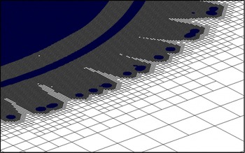
In the current approach, there are two main computational features associated with the AMR method. First, a cell-based isotropic refinement method is implemented in the Eulerian framework. A coarse cell is split into eight equal-size children cells in three dimensions. Second, due to the cell-by-cell adaptation, the AMR method results in an unstructured grid system. As shown in figure 5, the cell-based approach can dynamically refine the Eulerian grid at the moving phase boundaries with high flexibility, which provides more efficient grid management than a block-based AMR method (MacNeice et al. Reference MacNeice, Olson, Mobarry, de Fainchtein and Packer2000; Gunney, Wissink & Hysom Reference Gunney, Wissink and Hysom2006; Deiterding Reference Deiterding2009). Moreover, there is no grid nesting, overlapping, and level-level interpolation in a time step such that we do not require the cross-processor communication due to the inter-level interpolation. In addition, since there is no grid hierarchy, the data-fetching speed is faster than the octree type AMR (Agbaglah et al. Reference Agbaglah, Delaux, Fuster, Hoepffner, Josserand, Popinet, Ray, Scardovelli and Zaleski2011; Burstedde, Wilcox & Ghattas Reference Burstedde, Wilcox and Ghattas2011). The performance of fluid flow solver is independent of the total number of refinement level and less sensitive to the number of processors used.
Seven-level refinement around complex gas–liquid boundaries. The darkest (blue online) regions indicate the zones of liquid phase. The cell-based unstructured AMR approach can provide high flexibility and efficiency on grid management for such problems.

Grid adaptation is based on the location of interfaces and solution gradient on the Eulerian partitions. Geometry-based adaptation promotes a Cartesian grid around the neighbourhood of interfaces to the finest-level grid. The width of the finest refined region is five times that of the finest cell width on each side of the interfaces. Cells far away from the interface are adapted based on the solution of the flow field. The decision to refine or coarsen a cell is determined by comparing the vorticity magnitude
 ${\it\zeta}_{i}$
of a cell to the standard deviations of vorticity magnitude of the entire Eulerian domain
 ${\it\sigma}_{s}$
as
 $$\begin{eqnarray}\displaystyle \left.\begin{array}{@{}l@{}}{\it\xi}_{i}=\left|{\it\omega}_{i}\right|=\left|\boldsymbol{{\rm\nabla}}\times \boldsymbol{u}_{i}\right|,\ \text{cell }i\in {\it\Omega}_{p}\\ \displaystyle {\it\sigma}_{s}=\sqrt{\left(\mathop{\sum }\limits_{p=1}^{n}\mathop{\sum }\limits_{i=1}^{m}({\it\xi}_{i,p}-\bar{{\it\xi}})^{2}\right)/N}\\ \text{if }{\it\xi}_{i}>{\it\sigma}_{s}\text{ or }\left|\boldsymbol{x}_{i}-\boldsymbol{X}\right|<5{\rm\Delta}x,\ \text{refine cell }i\text{ to the highest level}\\ \text{if }{\it\xi}_{i}<0.2{\it\sigma}_{s},\text{ merge cell }i\text{ with neighbours if allowed.}\end{array}\right\} & & \displaystyle\end{eqnarray}$$
Mesh adaptation is triggered if the vorticity level within a computational cell is more than the standard deviation of the global vorticity strength. This criterion helps focus the available computational resource in regions where higher resolutions are required. Here,
 $i$
is the cell index of a partition
 ${\it\Omega}_{p}$
and
 ${\rm\Delta}x$
is the finest-level cell width.
We discussed the grid generation algorithm, domain repartition and data migration in Kuan (Reference Kuan2013). Interested readers can find the details of implementation in that paper. Recently, in a paper by Chen & Yang (Reference Chen and Yang2014), a thickness-based adaptation for multiphase flows is proposed to increase prediction accuracy for high-Weber-number flows. The results presented by Chen & Yang (Reference Chen and Yang2014) have highlighted the global flow structures in high-Weber-number regime. Their method allows an interface to moving around the computational domain, but it is not necessarily in regions covered by the finest grid. As a result, if the interface is in the coarser grid region, the varying interface thickness can affect the computational accuracy. Hence, these authors propose an additional criterion for adaptation to improve prediction around the interfacial region. In our approach, the phase boundary is by design always surrounded by the finest grid. Therefore, the interface thickness only depends on the finest grid resolution.
3.5. Experimental validation
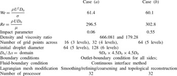
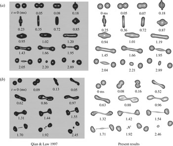
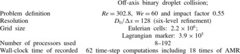
We validate our implementation by comparing numerical results of droplet collision at low Weber number with the experimental work of Qian & Law (Reference Qian and Law1997). The conditions of collision, the grid resolution, the computational domain and boundary condition setup are given in table 2. These two cases have similar Weber number and Reynolds number; but the histories of morphological change are very different due to the impact parameter. The impact parameter is the ratio of the distance between the centres of droplets projected in the direction normal to the relative movement of two droplets and the droplet diameter, which describes how case (a) is a near head-on collision. The droplets merge into a single droplet and then the merged body breaks into three secondary droplets after a cycle of radial-to-axial deformation. Case (b) is off-centre collision. The merged droplet stretches and twists for a while, and then evolves into a two-head body with an elongating ligament connecting the two bulkheads and ends up with multiple secondary droplets. Using the same front-tracking approach without parallel computational capabilities, Singh & Shyy (Reference Singh and Shyy2007) reported cases with conditions resulting in droplet coalescence, based on experiments of Qian & Law (Reference Qian and Law1997), at modest Weber numbers, accounting for coalescence and separation. Our results have reconfirmed such agreement detailed by Singh & Shyy (Reference Singh and Shyy2007).
Computational set-up of droplet collision at low Weber number. Reynolds number and Weber number are based on the liquid density
 ${\it\rho}$
, viscosity
 ${\it\mu}$
, surface tension coefficient
 ${\it\sigma}$
, initial droplet diameter
 $D_{0}$
and relative impinging speed
 $U$
.

Figure 6 shows the collision histories of cases (a) and (b) from experiments and computations in the left and right columns, respectively, with real-time notation. Overall, the morphologies are highly comparable between the computation and the experiment. Some discrepancies in the orientation and size of satellite droplets can be observed; they seem to be caused by multiple factors, including the sensitivity to the uncertainty of the initial conditions in the experiment, such as the relative velocity, offset of the path, angle of views, as well as numerical inaccuracy. To further address the accuracy of the methodology, in the following we perform a convergence test based on various mesh resolutions.
Binary droplet collision history at (a)
 $\mathit{We}=61.4$
,
 $\mathit{Re}=296.5$
and impact parameter 0.06; (b)
 $\mathit{We}=60.1$
,
 $\mathit{Re}=302.8$
, and impact parameter 0.55. Numerical results are computed with the resolution
 $D_{0}/{\rm\Delta}x=64$
.

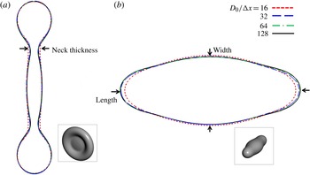
In order to perform a sensitivity analysis for the grid resolution, case (a) is repeated for four sets of grid resolution, i.e.
 $D_{0}/{\rm\Delta}x=16$
, 32, 64 and 128. The interface profiles at the cut plane
 $y=0$
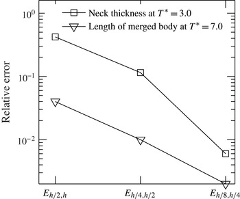
are overlapped to show discrepancies. Relative error is evaluated based on the deviation of the characteristic thickness or length,
 $l$
, of the merged droplet of coarser grid solution from the finer grid solution, as formulated in
 $$\begin{eqnarray}\displaystyle \text{E}_{h/2,h}=\text{abs}(l_{h/2}-l_{h})/D_{0}. & & \displaystyle\end{eqnarray}$$
The arrow markers in figure 7 denote the neck thickness used in the error estimation at dimensionless time
 $T^{\ast }=3.0$
or the length of the merged droplet at
 $T^{\ast }=7.0$
. Here
 $h$
denotes the solution at the grid
 $D_{0}/{\rm\Delta}x=16$
. The numerical error plot, figure 8 concludes that the simulation of the off-axis droplet collision at low Weber number converges with accuracy between first and second order.
Interface profiles on
 $y=0$
cut plane at (a)
 $T^{\ast }=3.0$
and (b)
 $T^{\ast }=7.0$
. The results from four resolution set-ups are represented by red, blue, green and black lines for the grid
 $D_{0}/{\rm\Delta}x=16$
, 32, 64 and 128, respectively.

Error of the neck thickness and length of the merged body.

3.6. Performance
We investigate the parallel performance of the field-equation solver, AMR and the interface-tracking method. These numerical experiments were conducted on the NYX machine at the Center of Advance Computing, University of Michigan. We used the nodes that consist of 240 Intel Nehalem Xeon E5540 CPU with InfiniBand networking.
The performances of the field-equation solver for the lid-driven cavity flow problems with grid size
 $1.6\times 10^{5}$
,
 $1.0\times 10^{6}$
and
 $4.0\times 10^{6}$
cells are evaluated without dynamic AMR. The linear solver used is the general minimal residual method (GMRES) with a Jacobi preconditioner (Balay et al.
Reference Balay, Brown, Buschelman, Eijkhout, Gropp, Kaushik, Knepley, McInnes, Smith and Zhang2012). Since the linear system of a discretized Poisson equation depends on the partition graph, the required iteration number reaching a prescribed rounding error for convergence varies with the number of processors used. In order to control the workload spent on solving a linear system on a varying number of processors, the wall-clock time of solving the Poisson equation is evaluated based on a fixed iteration number of the linear solver. We average the wall-clock time for 10 time-step computation and calculate the speedup based on the single processor computation for grid size
 $1.6\times 10^{5}$
and
 $1.0\times 10^{6}$
, and an eight-processor computation for grid size
 $4.0\times 10^{6}$
.
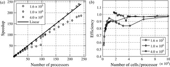
The performance of parallelization is determined by the computation-to-communication ratio and the cache hit rate. For a fixed-size problem, if we increase the number of processing unit, we decrease the computation-to-communication ratio that results in the slowdown of speedup. Figure 9(a) gives the speedup of these three cases. Due to decreasing computation-to-communication ratio, speedup slows down with the increasing number of processors. On the other hand, the effect of cache hit rate has an opposite influence on the efficiency: the finer the grain, the higher the hit rate of cache memory and then better efficiency. In case the entire working data set cannot fit into the cache, we can improve the parallel efficiency by using more processing units. This phenomenon is observed for the problem of grid size
 $4.0\times 10^{6}$
. A computation of larger processor count outperforms a computation with smaller processor count because of the effect of cache memory. This problem has the working data of a linear system solver that is excessively larger than the 8 MB L3 cache and results in a significantly low cache hit rate that overestimates the speedup of multiple-CPU computation. Figure 9(b) is the parallel efficiency based on the number of cells per processor. The flow solver shows the best efficiency at
 $1.0{-}2.0\times 10^{4}$
cells per processor on the computational platform specified. If we use a large number of cells per processor, we maintain efficiency around one but may have an unfavourable cache hit rate.
(a) Speedup of the field-equation solver for grid sizes
 $1.6\times 10^{5}$
,
 $2\times 10^{6}$
and
 $4\times 10^{6}$
. (b) Parallel efficiency as a function of number of cells/processor. The best usage of computational power is at 10 000–20 000 cells per processor. This range is determined by the computation-to-communication ratio and cache size of a system.

We use the example of the binary droplet collision to illustrate the overall performance of current approach. The investigation concentrates on the parallel performance of the AMR, interface-tracking method and field-equation solver. The performance is highly influenced by the effectiveness of the decomposition of the Eulerian and Lagrangian domains and communication. The computational set-up of this test is shown in table 3.
This is a strong scalability for an initial grid of
 $2.2\times 10^{6}$
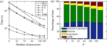
cells with a six-level refinement for 62 time steps. AMR operation invokes geometry-based adaptation around the Lagrangian interfaces at every 4 time steps and solution-based adaptation at every 20 time steps in the run-time. We analyse the performance based on this computational classification as Lagrangian tasks (interface shape modification), Eulerian–Lagrangian tasks (surface-tension computation, marker movement and material determination), Eulerian task (Cartesian-grid solver) and AMR. We present the usage of the wall-clock time in figure 10.
(a) Execution time of the Eulerian–Lagrangian method for a binary droplet collision computation. The original grid size is
 $2.2\times 10^{6}$
. Overall efficiencies are 0.65 and 0.48 on 64 and 128 processors, respectively. Procedures are categorized into four task groups. Eulerian (E): the field-equation solver; Eulerian–Lagrangian (E–L): the marker movement, cell material determination, and surface tension computation; Lagrangian (L): the interface shape modification; AMR: the AMR. (b) Breakdown of execution time of the Eulerian–Lagrangian method for a binary droplet collision computation.

Conditions and parameters of the performance test using adaptive Eulerian–Lagrangian interface tracking method.

The Eulerian task shows the best performance for its highest computation-to-communication ratio among all tasks. The speedup of AMR levels off after 32 processors as the computational time of AMR occupies 4–13 % of the total wall-clock time. The lowest computation-to-communication ratio of AMR is the reason of the lowest efficiency; and serialization and load imbalance due to localized adaptation around the interface are the overhead of AMR as well.
The time spending on Lagrangian tasks is 5–10 % of the total wall-clock time; and the speedup levels off at 128 processors. Of all the tests, every processor has a part of the Lagrangian interface, but the Lagrangian computation is imbalanced. Although the load imbalance of the Lagrangian task results in performance degradation, it is not the primary bottleneck of the overall scalability due to its low computational cost. We observe that the critical overhead is from the Eulerian–Lagrangian tasks. The Eulerian–Lagrangian tasks use 40–43 % of the wall-clock time, and show lower speedup than the Eulerian task because of the lower computation-to-communication ratio. Moreover, since Eulerian–Lagrangian tasks require communication for the Eulerian and Lagrangian domain coupling, their performance are highly related to the data size, number of messages and pattern of communication. The current domain decomposition of the Lagrangian requires the least communication for the coupling of the Eulerian grid and the Lagrangian element because exchanging data is right in the neighbourhood of subdomains. The efficiency of Eulerian–Lagrangian tasks and the overall performance can be optimized as the number of processors used increases.
In summary, the parallel performance of each group is proportional to its computation-to-communication ratio, in a descending order as Eulerian, Eulerian–Lagrangian, Lagrangian and AMR. This observation suggests that for a fixed-size problem, which is this parallel, adaptive interface-tracking method has an upper bound in efficiency, i.e. the performance of the Eulerian task. An ideal load-balanced algorithm for the Lagrangian interfaces will not so much benefit the overall performance due to the low computational cost of Lagrangian tasks. In contrast, the communication due to Eulerian–Lagrangian coupling is the primary overhead for large problems or processor counts.
4. Head-on binary droplet collisions in the high-Weber-number regime
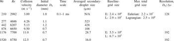
We have conducted a series of numerical simulation for droplet collision problems with high Weber number based on the conditions of experimental work of Pan et al. (Reference Pan, Chou and Tseng2009). Table 4 shows these parameters, initial droplet size and collision velocity, and experimental and numerical requirements. The materials are air at room temperature and water with surface tension coefficient
 $0.065\ \text{N}\ \text{m}^{-1}$
, density
 $998\ \text{kg}\ \text{m}^{-3}$
and viscosity
 $0.01\ \text{N}\ \text{m}^{-2}\ \text{s}^{-1}$
. The range of Weber number is from 200 to 1500 and the Reynolds number is from
 $2\times 10^{3}$
to
 $8\times 10^{3}$
. The physical length scale of initial droplet is approximately
 $1\ \text{mm}$
diameter, and the secondary droplet size ranges from 0.5 mm to
 $16\ {\rm\mu}\text{m}$
according to the simulation results. The resolution used is up to 192 grid points across the diameter of droplets. The total Eulerian grid size and number of Lagrangian markers are up to 22 million and 2.5 million, respectively, for case of
 $\mathit{We}=1520$
. The cell-based unstructured AMR effectively manages the computational resources with moving boundaries at run time. This case uses seven-level refinement on a
 $20D_{0}\times 20D_{0}\times 20D_{0}$
domain, where
 $D_{0}$
is the diameter of a droplet. For an equivalent grid resolution, a simulation using a uniform grid would require approximately 56 billion Eulerian cells.
The velocity, physical length and time scale of the experiments, and the numerical resources used in the computation.

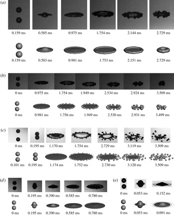
Figure 11 shows the snapshots of the colliding droplets compared with the experimental images adopted from Pan et al. (Reference Pan, Chou and Tseng2009). The impinging flow from both sides of two droplets extrudes a circular sheet at the waist of the merged body and expands with a growing rim at the fringe of the sheet. When the circular sheet is expanding, perturbations along the periphery of the rim (longitudinal direction) are observed. Surface tension effects may generate finger-like structures and further break the rim into satellite droplets. The diameter of the extruding sheet, instability pattern, size and distribution of satellite droplets are qualitatively comparable with the experimental results.
The collision history under different conditions. The numerical works are shown underneath experimental images at the corresponding physical time. Experiment pictures are adopted from Pan et al. (Reference Pan, Chou and Tseng2009). The computations of case (d) and (e) stop at earlier time steps because the required memory size exceeds the capability of the computational platform, which is 4 GB per processor: (a)
 $\mathit{We}=210$
,
 $\mathit{Re}=2890$
; (b)
 $\mathit{We}=277$
,
 $\mathit{Re}=4686$
; (c)
 $\mathit{We}=442$
,
 $\mathit{Re}=6207$
; (d)
 $\mathit{We}=878$
,
 $\mathit{Re}=6650$
; (e)
 $\mathit{We}=1520$
,
 $\mathit{Re}=8750$
.

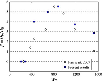
Figure 12 shows the breakup diameter normalized by initial droplet diameter
 $D_{0}$
versus Weber number. The breakup diameter is the diameter of the circular sheet at the moment of the primary (first-time) disintegration of the merged droplet. Compared with the experiments, the general trend is reasonably predicted by the computation. However, the simulated cases of
 $\mathit{We}=442$
and 878 show slightly larger breakup diameters. The discrepancy is possibly due to the temporal resolution of the topological change in both the experiment and the computation. The breakup in the computation is an artificial operation triggered when the characteristic length of the interface is smaller than the grid resolution
 ${\rm\Delta}x$
, leading to the exact timing of the topological variation. The case
 $\mathit{We}=1520$
has a larger breakup diameter than that measured in the experiments. The ‘prompt splattering’ that emits multiple droplets immediately after the impact is not observed in the numerical simulation, likely due to insufficient grid resolution, which demands more as the secondary droplets become smaller. The case of
 $\mathit{We}=1520$
is computed with a grid with resolution
 ${\rm\Delta}x=D_{0}/192$
. Apart from this case, the shape and size of droplets after breakup is consistent with experimental work. Again, further refined computations are limited by the capabilities of the available hardware.
The breakup diameter versus Weber number. The experimental data are reproduced from Pan et al. (Reference Pan, Chou and Tseng2009).

4.1. Summary of interface evolution
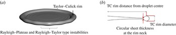
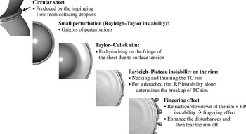
The collision starts with coalescence of the impacting droplets for all conditions. Bouncing does not happen since surface tension is relatively small in the high-Weber-number regimes. As the two droplets merge and continue to squeeze each other, a circular sheet evolves in the radial direction of the impinging plane. The circular sheet expands in a nearly axisymmetric manner with growing perturbations on its periphery. A circular rim at the fringe of the circular sheet gradually grows due to the end-pinching effect of the surface force, which is so-called Taylor–Culick rim (TC rim) (Taylor Reference Taylor1950, Reference Taylor1959; Culick Reference Culick1960). Figure 14 shows the structure of the TC rim with the circular sheet.
Disturbances along the rim are progressively amplified. For conditions of lower inertia, such as
 $\mathit{We}<1000$
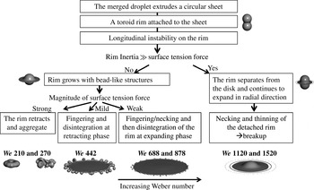
, the diameter of the rim increases as long as the circular sheet and the rim are connected. Thinning and necking happen to be a nodule-like structure due to the surface tension forces that occur along the longitudinal direction and shape the TC rim. This is a typical process of Rayleigh–Plateau (RP) instability (Strutt & Rayleigh, Reference Strutt and Rayleigh1878, Zhang et al., Reference Zhang, Brunet, Eggers and Deegan2010). Furthermore, the rim and sheet may retreat at later time, and the retraction of the circular sheet together with the necking effect on the rim isolate the nodule-like structures, which is so-called ‘fingering’ as shown in figure 11(c). The fingering makes the rim break into liquid ligaments or smaller secondary droplets. In the cases of high-inertia collision, such as
 $\mathit{We}=1176$
and 1520, the rim separates from the circular sheet at an early stage since surface energy cannot account for such high kinetic energy of the rim. The RP instability alone determines the evolution of first-time breakup process (figure 11
e). A summary of the overall interface evolution for Weber number from 200 to 1500 is shown in figure 13.
Summary of the interface evolution.

Generally, the processes of droplet collision are coalescence, deformation, amplification of disturbances and breakup. The global outline of the merged droplet linearly evolves with respect to time at the initial coalescence stage, especially before the extrusion of the circular sheet. The process is consistent with the conclusion of Roisman, Berberović & Tropea (Reference Roisman, Berberović and Tropea2009) in that for high enough Weber and Reynolds numbers, the flow far from the sheet edge generated by droplet collision is universal, almost independent of Weber and Reynolds number. On the other hand, the surface tension effects such as end-pinching and fluid viscosity determine the characteristics of TC rim and circular sheet.
4.2. Dynamics of the circular sheet and the TC rim
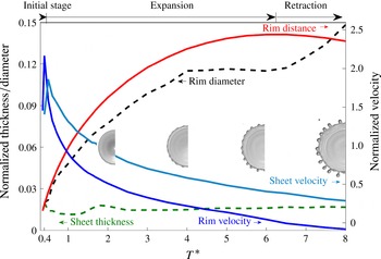
The TC rim velocity and circular sheet velocity are measured at the centre and the neck of the TC rim as shown in figure 14. In order to illustrate the interface evolution of the colliding droplet in the high-Weber-number regime, we use figure 15 to illustrate the velocity, diameter, the distance of the TC rim and the velocity and thickness of the circular sheet at the rim neck of the case
 $\mathit{We}=442$
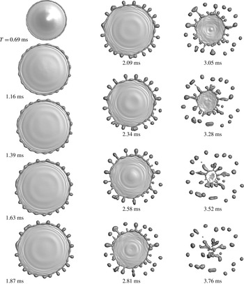
. This picture presents typical phenomena including the expansion, retraction and fragmentation of the TC rim due to longitudinal instabilities and fingering effect. A top view of the interface by the numerical result is given in figure 16.
The circular sheet and Taylor–Culick rim with longitudinal instabilities. The profile of a merged droplet on the right-hand side shows the characteristic length of the TC rim diameter, distance from the droplet centre to the rim centre, and the circular sheet thickness at the rim neck. In this case, for
 $\mathit{We}=442$
, the smallest sheet thickness is
 $3.84{\rm\Delta}x$
. The evolution of the corresponding length scales is shown in figure 15. While the resolution is insufficient to resolve the smallest sheet thickness, the overall dynamics presented in this case is reasonably captured.

Distance, thickness and velocity of the rim and the sheet of case
 $\mathit{We}=442$
. Representative snapshots at
 $T^{\ast }=2.0{-}8.0$
show the location of TC rim and longitudinal instabilities on the rim. Length scale and velocity are normalized by initial droplet diameter and relative colliding speed, respectively.

The top view of the interface evolution of case
 $\mathit{We}=442$
.

The development of the TC rim can be highlighted in three phases. First, the TC rim expands for a while, and then retracts back by surface tension forces if the rim is still attached to the circular sheet. Second, the diameter of the TC rim grows as it propagates. The increasing size of the TC rim is related to the velocity difference at the centre of the rim and the sheet velocity. Due to the surface tension force at the edge of circular sheet, the TC rim moves slower than the sheet that results in liquid accumulation in the TC rim. Third, there is a longitudinal instability on the TC rim. The evolution of the longitudinal (along-the-edge) disturbances can be antisymmetric perturbations of the Rayleigh–Taylor (RT) instability and symmetric perturbations governed by the RP instability (Strutt & Rayleigh Reference Strutt and Rayleigh1878; Agbaglah, Josserand & Zaleski Reference Agbaglah, Josserand and Zaleski2013).
The interface evolution: instabilities on the edge of the circular sheet.

At the initial stage of collision, the circular sheet quickly decelerates while expanding. The circular sheet is continually thinning and expanding with the growing TC rim. The deceleration of TC rim is very strong right after the sheet extrusion, but weakens quickly later. As a result, the RT-type instability may be profound at the beginning of collision. At the expansion and retraction stage, the deceleration is relatively small such that the effect of RT instability fades away. The TC rim propagates at lower speed than the circular sheet due to surface tension force at the edge. In the long time, we observe the nearly symmetrical, wavy structure along the rim periphery. The RP instability dominates the growth of the longitudinal disturbances since the growth rate of RP type is much faster than the RT type. After the onset of RP instability on the rim, the largest-amplitude wavenumber will not change much, and eventually determine the number of secondary droplets of the primary breakup.
On the liquid sheet, capillary waves appear behind the TC rim. When the rim and the liquid sheet expand, the capillary wave exhibits axisymmetric propagation. At the retraction stage, the TC rim confines the capillary wave in a reducing space. The capillary wave gradually interacts with each other, and then breaks the symmetry. The interaction becomes more violent and eventually triggers rupture of the liquid film, as shown at the snapshot at
 $T=3.28$
of figure 16. The propagation of capillary waves at the rim expanding stage shows similarities to the work of Song & Tryggvason (Reference Song and Tryggvason1999), which resolves fluid sheet retraction computationally by a two-dimensional front-tracking method. The magnitude of capillary waves on the retracting liquid sheet is related to the Ohnesorge number (
 $\mathit{Oh}={\it\mu}/\sqrt{{\it\rho}{\it\sigma}l}$
, where the length scale
 $l$
can be the diameter of droplets), for accounting momentum dissipation effect of viscous fluids. The influence of fluid viscosity at the capillary wave on two-dimensional fluid sheet have been discussed by Savva & Bush (Reference Savva and Bush2009). Three-dimensional film rupture and capillary waves produced by the head-on droplet collisions will be explored in the future.
Figure 17 is a summary to the history of the longitudinal instabilities on the edge of the circular sheet. At the initial stage of collision, the merged body ejects a high-speed liquid sheet radially on the impinging plane. This circular jet quickly decelerates, and the initial disturbances on the edge of the sheet are likely due to the RT-type instability. The TC rim grows and propagates at lower speed than the circular sheet. In the long time, the RP instability takes over the growth of the longitudinal disturbances. After the onset of RP instability, we see progressive growth of the disturbances. At later stage, the retraction or slowdown of the TC rim amplifies the irregularity of the dominant disturbance due to RP instability. This yields the fingering structure that disintegrates the TC rim eventually. If the collision speed is high enough, the TC rim detaches from the main droplet before the build-up of the longitudinal instability.
4.3. Primary breakup and secondary-droplet size
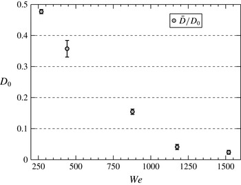
Figure 18 shows the size of secondary droplet as a function of global Weber number. The diameter and velocity of the secondary droplet are calculated by measuring droplet diameter directly. When a droplet is an ellipsoid, we calculate the equivalent diameter of droplet by measuring its three semi-principle axes based on volume equivalence. For the conditions of the present study, the deterministic factors of the secondary droplet diameter are the dominant wavenumber on the TC rim, rim thickness and the breakup mechanism.
The average secondary droplet size relative to
 $D_{0}$
with respect to Weber number.

In cases of a uniform liquid jet, the surface tension forces break the liquid thread into a series of secondary droplets and liquid ligaments between the main drops. These ligaments become spherical eventually. One may use the most pronounced wavenumbers on the liquid thread and volume conservation to estimate the droplet size distribution (Ashgriz & Yarin Reference Ashgriz, Yarin and Ashgriz2011). Zhang et al. (Reference Zhang, Brunet, Eggers and Deegan2010) suggested that we can correlate the secondary droplet size for crown splashing problems with the dominant wavenumber on the rim. For a simplified problem as considered by Strutt & Rayleigh (Reference Strutt and Rayleigh1878), the dominant wavenumbers on a circular thread due to surface tension forces is a function of the diameter of the rim. In the present cases, the diameter of the TC rim is time-dependent and the onset timing of RP instability is unclear. Even more, the breakup mechanism affects the secondary droplet size as well. In some cases, the TC rim may start to break while the attached circular sheet is receding. The interaction of the receding sheet and RP instability leads to the fingering effect. A finger structure may coalesce with its nearby structures, which results in more complex scenarios than a simple breakup based on wavenumbers of the TC rim. This is the primary reason that in the case of
 $\mathit{We}=442$
, which has profound fingering effects, the standard deviation of the secondary droplet diameter is the largest among all cases.
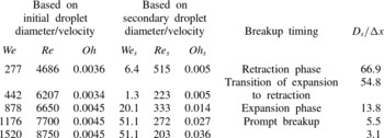
We list dimensionless parameters,
 $\mathit{We}_{s}$
,
 $\mathit{Re}_{s}$
and
 $\mathit{Oh}_{s}$
based on the averaged diameter and velocity of the secondary droplet of the primary breakup in table 5. Here
 $\mathit{We}_{s}$
of these cases is from 1.3 to 51.1. For the case of
 $\mathit{We}=277$
, the secondary-to-initial droplet size ratio is 0.48, as given by figure 18, but the corresponding Weber number ratio is more than 40. It indicates that the averaged velocity of the secondary droplets is approximately eight times the initial impinging velocity. In the case of
 $\mathit{We}=442$
, the primary breakup occurs at the transition of the sheet expansion to retraction. Most of the secondary droplets contain relatively low velocity, thereby showing the smallest
 $\mathit{We}_{s}$
. Below
 $\mathit{We}=878$
, where the breakup diameter
 ${\it\beta}$
is about the maximum (figure 12), both
 $\mathit{We}_{s}$
and
 $\mathit{Re}_{s}$
decrease with increasing
 $\mathit{We}$
since the secondary droplets are generated at the rim that is rendering less kinetic energy of retraction and the size becomes smaller. For the cases with high, initial kinetic energy (
 $\mathit{We}=1176$
and 1520), the secondary droplets propagate at much higher velocity than secondary droplets generated at the retraction phase (
 $\mathit{We}=277$
and 442). The increasing
 $\mathit{We}_{s}$
is due to higher kinetic energy per unit mass left in the secondary droplets for the higher
 $\mathit{We}$
cases.
The Weber, Reynolds and Ohnesorge number based on the secondary droplet scale of the primary breakup. The last column provides average secondary droplet size
 $D_{s}$
, normalized by the grid resolution
 ${\rm\Delta}x$
.

Here
 $\mathit{Oh}_{s}$
is 0.005 for cases 2 and 3, and jumps to order of
 $10^{-2}$
for higher
 $\mathit{We}$
cases. Judged by the magnitudes of
 $\mathit{Re}_{s}$
and
 $\mathit{We}_{s}$
, it appears that in this regime, for the secondary droplet dynamics, the viscous effect is secondary compared with the surface tension effect. However, as the length scales become smaller either during subsequent collision or toward the boundary of the droplet, the viscous effect will become more influential.
5. Conclusion
We have developed a parallel, adaptive Eulerian–Lagrangian interface-tracking method to simulate binary-droplet collision at high Weber number. The main challenge on parallelism is the dilemma between the load balance of Lagrangian computation and communication cost due to the Eulerian–Lagrangian coupling. The key is to minimize communication cost because the communication overhead is more severe than the imbalance of Lagrangian computation when increasing the grid size of a problem and the number of processing units.
The computation-to-communication ratio is the dominant factor on the efficiency of the Eulerian–Lagrangian interface-tracking method. The field-equation solver (Eulerian task) achieves the most efficient computation in a specific range of Eulerian-grid size per processor, with the details depending on the processor specifics. This range is a function of the computation-to-communication ratio and the grain size with respect to the shared cache size per CPU. On the other hand, the scaling analysis suggests that the load balance of the Lagrangian markers is not influential on the overall performance due to the relative low computation load.
The simulation of high-Weber-number droplet collision provides informative morphologies in space and time. In general, the processes of droplet collision are coalescence, deformation, amplification of disturbances and breakup. The global outline of the merged droplet linearly evolves with respect to time at the initial coalescence stage, especially before the extrusion of the circular sheet. The merging, expansion, end pinching, fingering, free surface instabilities and primary breakup of droplets are successfully resolved and consistent with experimental work. Insights of the interface evolution are summarized below.
-
(i) Disturbances along the rim are progressively amplified. The end-pinching effect due to surface tension force produces a TC rim on the edge of the circular sheet. The rim expands and may retract back at the later time with growing longitudinal instabilities.
-
(ii) Two types of longitudinal instabilities on the TC rim have been identified. The RT-type instability can be significant at the initial deceleration phase of the circular sheet right after droplet coalescence. Later, the RP instability takes over the growth of disturbances on the TC rim.
-
(iii) For
 $\mathit{We}<1000$
, the diameter of the rim increases as long as the circular sheet is connected with it. The fingering makes the rim break into liquid ligaments or smaller secondary droplets. For high-inertia collision, such as
$\mathit{We}=1176$
and 1520, the rim separates from the circular sheet at an early stage since surface energy cannot account for such high kinetic energy of the rim. Retraction and the fingering effect are not observed before the first-time breakup of the TC rim, and the RP instability alone determines the evolution of breakup process.
-
(iv) Three factors are observed which can significantly influence the secondary-droplet size: the rim thickness, the dominant wave of the rim, and the breakup timing. For the TC rim disintegrates at the retraction phase, the fingering effect is profound and results in wider droplet size distribution. If the breakup happens at the expansion phase of the rim, the size of secondary droplet is mostly determined by the dominant wave due to RP instability.


Acknowledgements
This work has been partially supported by NASA Constellation University Institutes Program (CUIP), Claudia Meyer program manager.