1. INTRODUCTION
Global Navigation Satellite Systems (GNSS) have an essentially unavoidable drawback. Their navigation receivers can be easily jammed or spoofed. Thus, other types of navigation devices are being developed. Computer vision systems are widely applied for the solution of motion control and navigation problems. Visual band cameras are comparatively small, lightweight and cheap. Nevertheless, such cameras are capable of realising high precision measurements. For instance, star trackers can determine angular orientation with errors of about 1–3 arc seconds. Unfortunately, the precision of visual shoreline navigation is much worse. This is due to the variability of the observed navigation object, their significant size and the presence of atmospheric distortions and obscuration. The atmosphere causes light absorption and light refraction and the shape of the observed shoreline can vary significantly. The variations of the shoreline shape are so great that the navigation errors cannot be replaced with averaged values. So, each navigation measurement should be accompanied with an individual error covariance matrix of measurements.
This paper constructs a Cramer-Rao lower bound for position estimation. Well-developed algorithms of visual navigation usually have errors which are near to this bound. A necessary condition for this is the approximately Gaussian law of the localisation error distribution of the shoreline segment, with the absence of “heavy tails” of distribution and the absence of anomalous errors.
2. STATE OF THE ART
Automatic image navigation algorithms are used to correct the orbital and attitude misalignment of geosynchronous satellites. Additionally, automatic matching of landmarks is used for the calibration and control of imagery geometry (Carr and Madani, Reference Carr and Madani2007). Landmarks are formed from the Global Self-consistent Hierarchical High-resolution Shoreline (GSHHS) database (GSHHG, 2017; Wessel and Smith, Reference Wessel and Smith1996). It should be mentioned that similar automatic image navigation algorithms can function on board in real time provided that there is a sufficiently powerful processor.
The tasks involved in Earth image automatic map registration are close to the tasks of navigation. Registration tasks of satellite images to different vector maps are significantly widespread (Fujii and Arakawa, Reference Fujii and Arakawa2004; Madani et al., Reference Madani, Carr and Shoeser2004; Wang et al., Reference Wang, Stefanidis, Croitoru and Agouris2008; Habbecke and Kobbelt, Reference Habbecke, Kobbelt and Kutulakos2012; Li and Briggs, Reference Li and Briggs2006; Zeng et al., Reference Zeng, Fang, Ge, Li and Zhang2017). Fujii and Arakawa (Reference Fujii and Arakawa2004) introduced a fully automatic method for registering satellite images to vector maps in urban areas. Madani et al. (Reference Madani, Carr and Shoeser2004) presented a fully automatic real-time landmark image registration based on matching a measured landmark to the corresponding shoreline landmarks extracted from a digital map. Wang et al. (Reference Wang, Stefanidis, Croitoru and Agouris2008) proposed a fast automatic algorithm for registering aerial image sequences to vector map data using linear features as control information. Habbecke and Kobbelt (Reference Habbecke, Kobbelt and Kutulakos2012) investigated the problem of a fully automatic and robust registration for oblique aerial images in cadastral maps. Li and Briggs (Reference Li and Briggs2006) proposed a new approach for automated georeferencing of raster images to a vector road network. Alignment of the latitude and longitude for all pixels for Geo-Stationary Meteorological Satellite (GSMS) images was considered by Zeng et al. (Reference Zeng, Fang, Ge, Li and Zhang2017). The shorelines of selected reference lakes were used as landmarks.
The shoreline is a unique object for navigation. With the exception of the circumpolar regions, the world's oceans do not freeze. A very small difference in the heights of world oceans greatly simplifies the task of recognising coastlines from a wide range of angles of observation and the position of the sun. In addition, the shorelines themselves have a high contrast in the red and near infrared range.
It should be mentioned that even for one section of the coastline, different angles and observation distances will result in different errors of navigation. For different segments of shorelines, the accuracy of navigation will differ even more. This is one of the essential features of optical navigation. For estimation of the navigation error, the Cramer-Rao lower bound can be used.
3. COORDINATE SYSTEMS
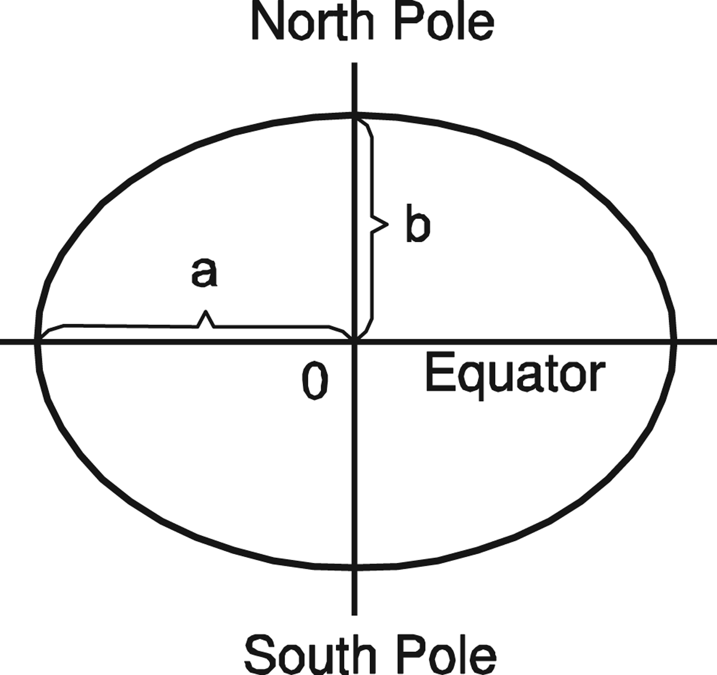
The World Geodetic System (WGS) 84 coordinate system will be used for navigation. The Earth is approximated by an ellipsoid as in Figure 1.
World Geodetic System ellipsoid; a – semi-major axis, b – semi-minor axis.

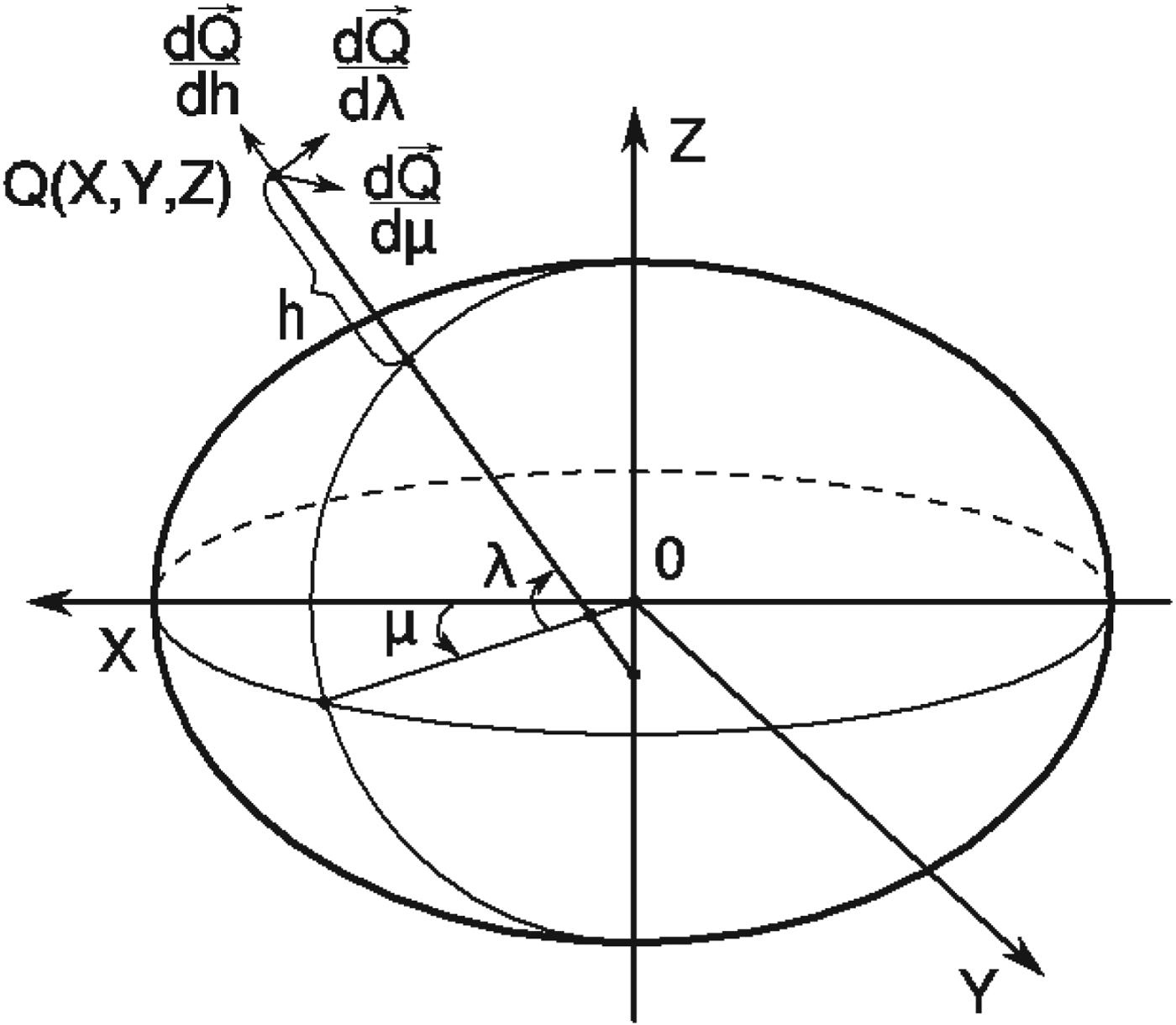
The position of any point in space is determined by three parameters - λ – latitude, μ – longitude and h – altitude over the ellipsoid surface (Equation (1)).
 $$\left\{\matrix{ X=\lpar N+h\rpar \cos \lambda \cos \mu \hfill \cr Y=\lpar N+h\rpar \cos \lambda \sin \mu\comma \; \hfill \cr Z=\lpar Nb^2/a^2+h\rpar \sin \lambda \hfill}\right. $$
where N is the prime vertical:
 $$N=\displaystyle{{a}\over{\sqrt{1-e^2\sin ^2\lambda}}}\comma \; $$
and e 2 is the first eccentricity:
 $$e^2=\displaystyle{{a^2-b^2}\over{a^2}} $$
The spatial rectangular coordinates of a camera expressed through geodetic coordinates are shown in Figure 2.
Axes of the camera's coordinate system.

The vectors of the camera coordinate system are now determined by using the differentiation operation. The camera is at point Q with coordinates Q = (X,Y,Z). The vectors are introduced:
 $${\bf e}_1^{\ast} =-\displaystyle{{d{\bf Q}}\over{dh}}\comma \; \quad {\bf e}_2^{\ast} =\displaystyle{{d{\bf Q}}\over{d\lambda}} \comma \; \quad {\bf e}_3^{\ast} =\displaystyle{{d{\bf Q}}\over{d\mu}} $$
 $$\eqalign{{\bf e}_1^{\ast} &=\left(\matrix{ -\cos \lambda \cos \mu \comma \; & -\cos \lambda \sin \mu \comma \; & -\sin \lambda }\right)\cr {\bf e}_3^{\ast} &=\left(\matrix{ -\lpar N+h\rpar \cos \lambda \sin \mu \comma \; & \lpar N+h\rpar \cos \lambda \cos \mu \comma \; & 0 }\right)} $$
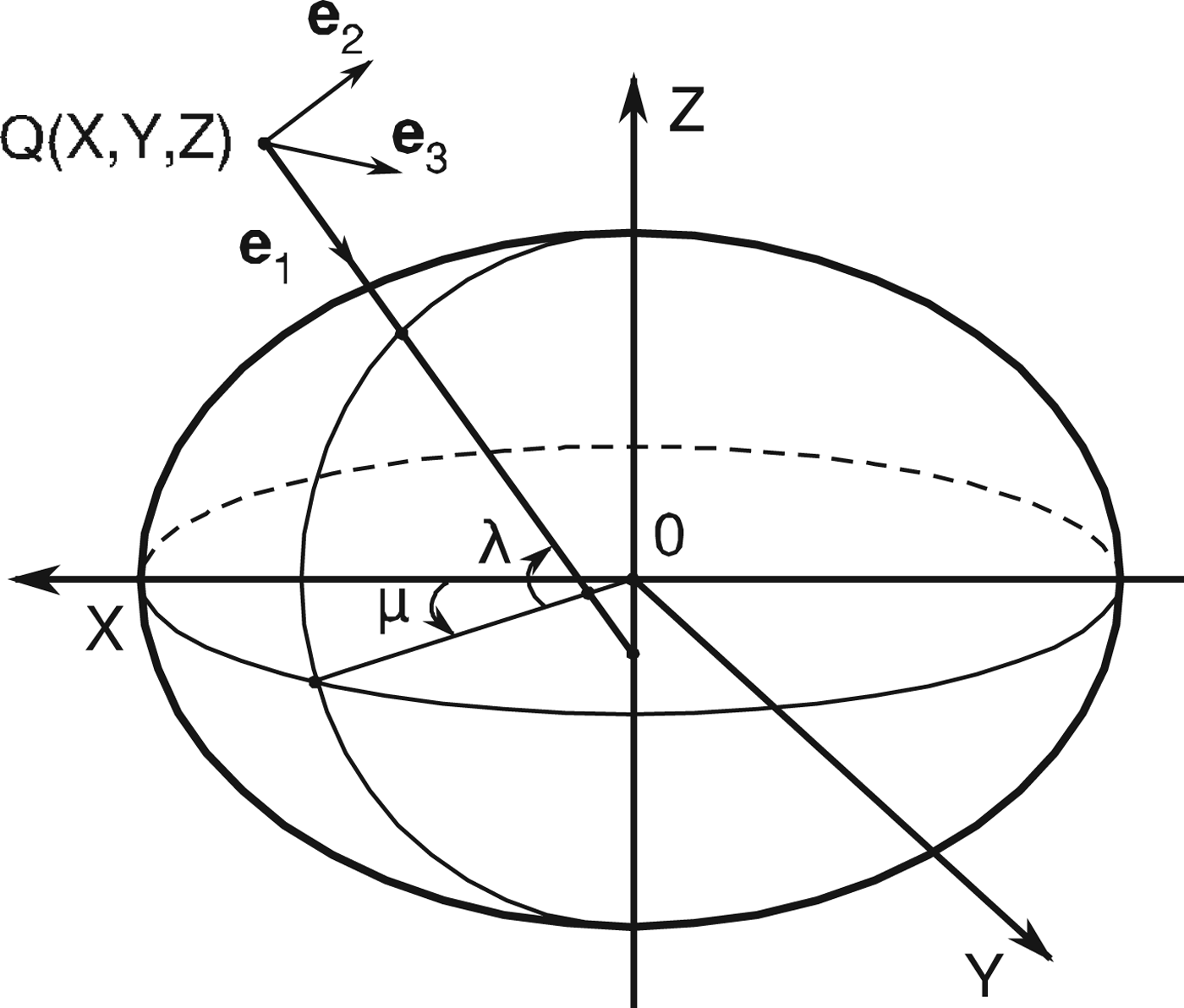
These vectors will be used to obtain orthonormal basis vectors  ${\bf e}_{1}$,
 ${\bf e}_{2}$ and
 ${\bf e}_{3}$ (Figure 3). Vector
 ${\bf e}_{2}$ can be more easily obtained from a vector product of
 ${\bf e}_{3}$ and
 ${\bf e}_{1} $. These
 ${\bf e}_{1} $ and
 ${\bf e}_{3}$ vectors are:
 $$\eqalign{{\bf e}_1 & =\displaystyle{{{\bf e}_1^{\ast}} \over{\vert{\bf e}_1^{\ast}\vert}}=\left(\matrix{ -\cos \lambda \cos \mu \comma \; & -\cos \lambda \sin \mu \comma \; & -\sin \lambda } \right)= \left(\matrix{ e_{11} \comma \; & e_{12} \comma \; & e_{13} } \right)\cr & \qquad \quad {\bf e}_3 = \displaystyle{{{\bf e}_3^{\ast}} \over{\vert{\bf e}_3^{\ast}\vert}}=\left(\matrix{ -\sin \mu \comma \; & \cos \mu \comma \; & 0 } \right)=\left(\matrix{ e_{31} \comma \; & e_{32} \comma \; & e_{33} } \right)} $$
Camera's coordinate system.

The vector  ${\bf e}_{2}$ is obtained as the vector product:
 $$\eqalign{ {\bf e}_2 &=\left\vert\matrix{ i & j & k \cr {e_{31}} & {e_{32}} & {e_{33}} \cr {e_{11}} & {e_{12}} & {e_{13}} }\right\vert=\left\vert\matrix{ i & j & k \cr {-\sin \mu} & {\cos \mu} & 0 \cr {-\cos \lambda \cos \mu} & {-\cos \lambda \sin \mu} & {-\sin \lambda} }\right\vert \cr & =\left(\matrix{ -\sin \lambda \cos \mu \comma \; & -\sin \lambda \sin \mu \comma \; & \cos \lambda } \right)} $$
So, vector  ${\bf e}_{1}$ is directed to the ellipsoid surface and orthogonal to it. The vector
 ${\bf e}_{2}$ is directed to the North Pole and lies in the plane which is parallel to the ellipsoid surface. The vector
 ${\bf e}_{3}$ is directed to the direction of increasing longitude and also lies in the plane which is parallel to the ellipsoid surface. It is easy to take into account the real angles of roll, pitch and yaw, but taking these angles into account will complicate further calculations and make them more difficult to understand.
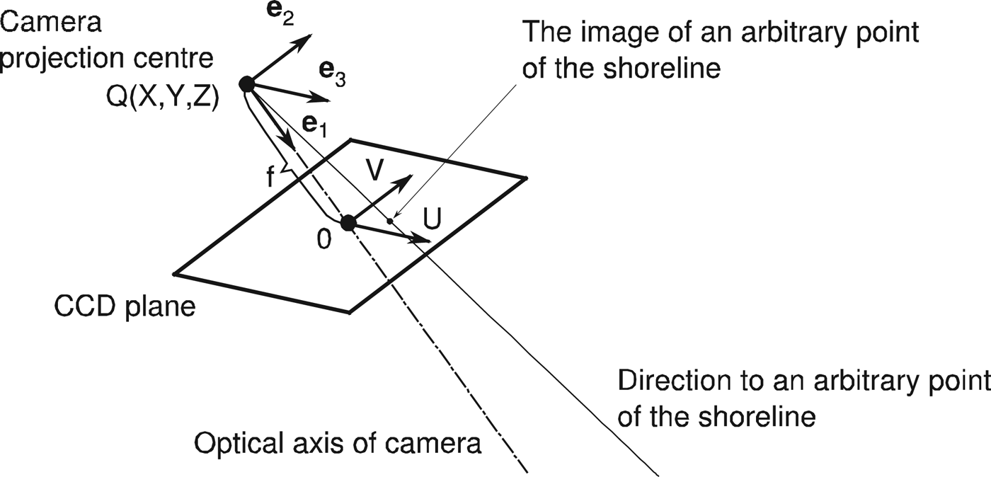
A relation between the coordinate systems of the camera (see Figure 3) and of the Charge-Coupled Device (CCD) matrix is shown in Figure 4. Here f is the focal length. U and V are the axes of the CCD matrix coordinate system. The vector  ${\bf e}_{1}$ coincides with the optical axis of the camera.
CCD matrix's coordinate system.

4. SHORELINE MAP IMAGE
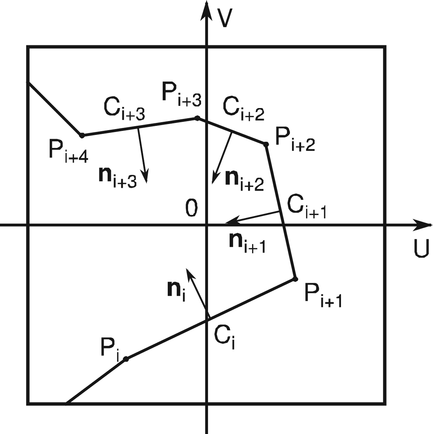
The shoreline map presents a sequence of segments which approximate a shoreline. The segments are represented by a sequence of points with coordinates of longitude and latitude. All contours are closed. The direction of contour bypass is counter-clockwise. An image of some segments is presented in Figure 5. The points Pi, Pi+1, Pi+2, Pi+3, Pi+4 are the ends of segments. Points Ci, Ci+1, Ci+2, Ci+3 are the midpoints of segments. Profiles of the brightness of the ocean/mainland are attached to these points. Normals ni, ni+1, ni+2, ni+3 are directed from the ocean to the mainland.
Segments of shoreline map.

The Global Self-consistent, Hierarchical, High-resolution Geography Database (GSHHG, 2017) maps include the World Vector Shorelines map. This map has five resolutions (full, high, intermediate, low and crude). Unfortunately, these maps have poor precision (Aksakal, Reference Aksakal2013; Baldina et al., Reference Baldina, Bessonov, Grishin, Zhukov and Kharkovets2016). Errors can vary from 50 to 500 m (Aksakal, Reference Aksakal2013). These errors should be eliminated at the stage of map preparation. Also, tidal corrections should be made at this stage.
5. MAXIMUM LIKELIHOOD METHOD
The error of shoreline localisation on the raster image of the Earth is approximated by the normal law, expressed in Equation (8).
 $$\eta \lpar x\rpar =\displaystyle{{1}\over{\sigma \sqrt{2\pi}}}\exp \left(-\displaystyle{{\lpar x-x_0\rpar^2}\over{2\sigma^2}}\right)$$
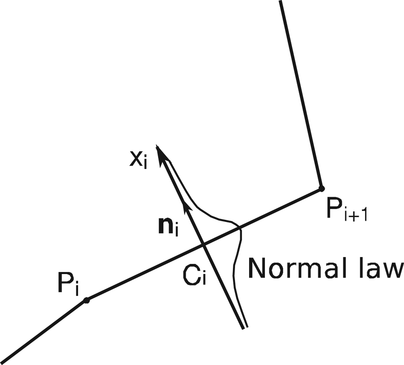
The error of the relative position of the map segment is measured in the normal direction to this image map segment. These errors of localisation are attributed to the midpoints of the segments (points Ci, Ci+1, Ci+2, Ci+3). The normal law graph of localisation errors attached to the midpoint of the shoreline image segment is shown in Figure 6.
Normal law of localisation error.

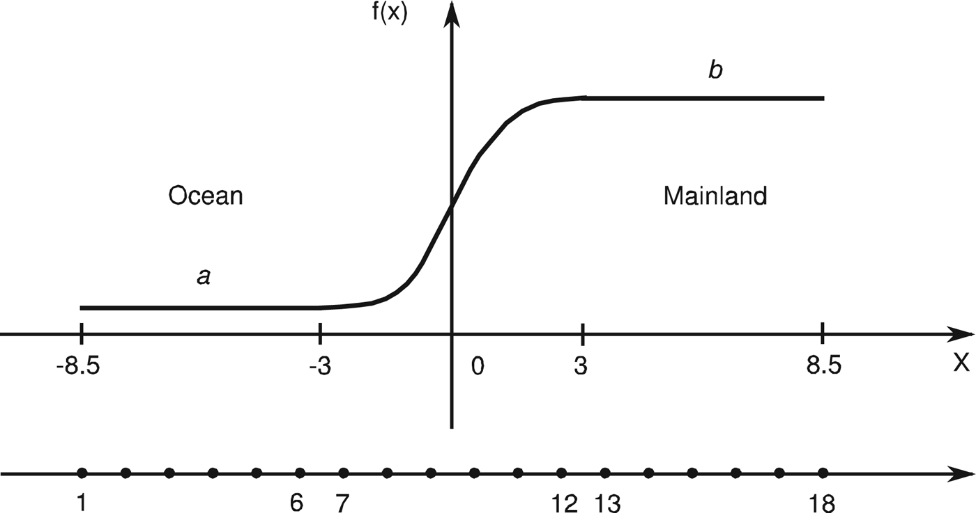
The parameters of the normal law are formed during the task of determining the navigation solution, which was done by alignment of the shoreline map with the shoreline raster image in two steps. The first step is a coarse alignment. After the first step, the alignment error between the vector shoreline map and the raster image of the shoreline does not exceed one pixel. At the second step (precision alignment), the shift between the calculated position of the map shoreline segments and the real shoreline position on the raster image is iteratively reduced by optimisation in the space of variables λ, μ and h. A special method is used for the estimation of the real shoreline position on the raster image. Let us briefly consider it. The brightness profile model on the border between an ocean and a mainland is presented in Figure 7. In the same figure, the brightness sample points of the raster image profile are marked 1–18. These points are located on a straight line perpendicular to the segment of the shoreline map.
Brightness profile model and brightness sample points.

The brightness profile model consists of two horizontal segments with brightness a (ocean) and b (mainland) and the transitional zone between them. The transitional zone is modelled by a spline of the third order. The middle of the transition zone is tied to the calculated position of the map shoreline segment. This model is described by four parameters (brightness of the ocean, brightness of the mainland, width of transition zone and shift along the OX axis). For localisation, it is advisable to use the maximum likelihood method, which simultaneously evaluates all four parameters. Estimation of these parameters requires searching for an extremum in four-dimensional spaces for all the map segments used for navigation. This task requires too much computational resource, especially for on board applications. For simplification of this task, the mean value of brightness of a (ocean) and b (mainland) is estimated as the average of values of brightness of samples 1–6 and 13–18. The width of the transitional zone depends on the effective point scattering function of the optical system and preliminary processing of images. For the images under consideration, this width was chosen to be equal to six pixels. In this way, only one parameter should be estimated by means of a search for an extremum. This parameter is the shift of the brightness profile model relative to the border between ocean and mainland on the raster image. The method of forming the brightness samples 1–18 will be considered later.
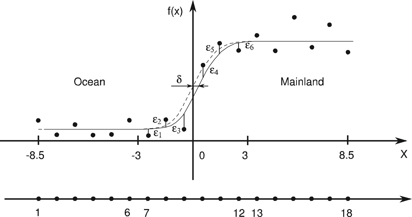
The relative shift δ of the brightness profile model and the real shoreline on samples 1–18 is estimated with a precision of 0·1 pixels by means of minimisation of the sum of the squares of the deviation of the model profile from the real profile – see Figure 8.
Estimation relative shift δ between the model profile and the real one. Points on the graph are the real brightness profile on the raster image.

In the transition zone, the residual deviations  $\varepsilon_{1} -\varepsilon _{6}$ of the real brightness profile from the model influence the error of relative shift estimation. These deviations are called the regressive residuals in regression analysis.
There is a very serious and complicated question of error localisation estimation for each individual segment. The fact is that the individual profiles of ocean/mainland brightness differ greatly. So, the localisation errors of the shoreline differ greatly too. Therefore, it is highly undesirable to use “average” estimates, which can be very far from reality. It is suggested to use regressive residuals for the estimation of localisation errors. The assumption of the independence of these residuals greatly simplifies the calculations of localisation errors, although it gives a somewhat overestimated value of the error estimate for localisation. In our case, the standard deviation of δ is estimated from a very simple formula:
 $$\sigma^2 =\displaystyle{{1}\over{\lpar b-a\rpar ^2}}\sum_{i=1}^6 \varepsilon_i^2 $$
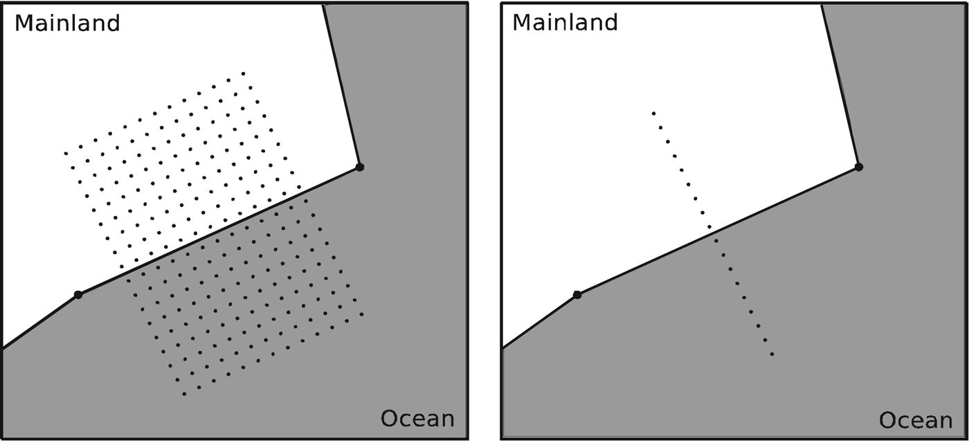
Consider how the brightness samples 1–18 are formed. Each segment of the shoreline map which is used for navigation generates a local coordinate system. One vector is directed along a segment, and another is directed orthogonal to this segment. In this coordinate system a grid of samples of brightness is built. The grid step size is selected in the order of one pixel or more (Figure 9, left image). The samples of brightness are formed by subpixel bilinear interpolation on the raster image.
A grid of samples in the vicinity of the segment (left image). Samples 1–18 of brightness profile (right image).

Then, all these samples are summarised in a direction parallel to the segment. So, samples 1–18 of brightness profile are obtained (Figure 9, right image).
It is necessary to consider map quality. The law expressed by Equation (8) is adequate provided there are no systematic errors in the map. Unfortunately, some fragments of GSHHG maps have significant systematic errors. Systematic errors condition the correlation of individual errors of the localisation of different segments and produce significant navigation errors. It is assumed that maps do not have systematic errors, so we can obtain a multi-dimensional function of segment error localisation for n segments (it is also a likelihood function for fixed  $\hbox{x}_{1}\comma \; \hbox{x}_{2}\comma \; \ldots\comma \; \hbox{x}_{n}\rpar $.
 $$f\lpar \brtheta \comma \; x_1 \comma \; x_2 \comma \; \ldots\comma \; x_n\rpar =\prod_{i=1}^n \displaystyle{{1}\over{\sigma_i \sqrt {2\pi}}} \exp \left(-\displaystyle{{\lpar x_i -x_{0i}\lpar \brtheta\rpar \rpar^2}\over{2\sigma_i^2}} \right)$$
The points  $x_{0i} \lpar \brtheta\rpar $ are calculated according to the map and taking into account the camera position and orientation. This is the “ideal” position of shoreline segments. The real position of the shoreline on the pixel image from the camera will differ from its “ideal” position. For each map segment, we measure a shift x i of the “real” ocean/land border relative to its “ideal” position in the normal direction to the map segment.
Here it is assumed that segment localisation errors are independent and have a normal distribution law. Error independence allows reduction of the multidimensional distribution density to the product of one-dimensional densities. Error independence is provided by the quality of the preparation of cartographic information.
Vector  $\brtheta=\lpar \lambda\comma \; \mu\comma \; h\rpar $ should be determined to solve the navigation task. This vector has three dimensions instead of six. In fact, rotation of the camera around two horizontal axes and the shift relative to this axis are strongly correlated. Thus, roll and pitch can be estimated by means of another sensor (for instance, a star tracker for spacecraft or high-altitude hypersonic unmanned aerial vehicle). In this case, it is also expedient to determine the remaining course angle (yaw) by means of a star tracker. The star tracker must be rigidly mechanically connected with the navigation camera. If it is necessary to expand the vector of the measured parameters, the information matrix can be easily obtained by analogy with the three parameters case.
The logarithm of the likelihood function is:
 $$\eqalign{ L\lpar \theta\comma \; x_1\comma \; x_2\comma \; \ldots\comma \; x_n\rpar & =\sum\limits_{i=1}^n \ln \left(\displaystyle{{1}\over{\sigma_i \sqrt {2\pi}}} \exp \left(-\displaystyle{{\lpar x_i -x_{0i}\lpar \brtheta\rpar \rpar^2}\over{2\sigma_i^2}} \right)\right)\cr & = -\displaystyle{{n}\over{2}}\ln \lpar 2\pi\rpar +\sum\limits_{i=1}^n \left(-\ln \sigma_i -\displaystyle{{\lpar x_i -x_{0i}\lpar \brtheta\rpar \rpar^2}\over{2\sigma_i^2}}\right)} $$
6. CRAMER-RAO LOWER BOUND AND FISHER INFORMATION MATRIX
The Cramer-Rao lower bound (Van Trees, Reference Van Trees2001) is expressed through the Fisher information matrix:
 $$Var\lpar \brtheta\rpar =\left(\matrix{ E\lpar \hat{\lambda} -\bar{\hat{\lambda}}\rpar^2 & E\lpar \hat{\lambda} -\bar{\hat{\lambda}}\rpar \lpar \hat{\mu} -\bar{\hat{\mu}}\rpar & E\lpar \hat{\lambda} -\bar{\hat{\lambda}}\rpar \lpar \hat{h}-\bar{\hat{h}}\rpar \cr E\lpar \hat{\mu} -\bar{\hat{\mu}}\rpar \lpar \hat{\lambda} -\bar{\hat{\lambda}}\rpar & E\lpar \hat{\mu} -\bar{\hat{\mu}}\rpar^2 & E\lpar \hat{\mu} -\bar{\hat{\mu}}\rpar \lpar \hat{h}-\bar{\hat{h}}\rpar \cr E\lpar \hat{h}-\bar{\hat{h}}\rpar \lpar \hat{\lambda} -\bar{\hat{\lambda}}\rpar & E\lpar \hat{h}-\bar{\hat{h}}\rpar \lpar \hat{\mu} -\bar{\hat{\mu}}\rpar & E\lpar \hat{h}-\bar{\hat{h}}\rpar^2 }\right)\ge {\bf I}_n^{-1} \lpar \brtheta\rpar \comma \; $$
where E is the sign of mathematical expectation,  $\hat{\lambda} \comma \; \hat{\mu} \comma \; \hat{h}$ are estimations of coordinates and
 $\bar{\hat{\lambda }}\comma \; \bar{\hat{\mu}}\comma \; \bar{\hat{h}}$ are the mathematical expectation of these estimations.
The Fisher information matrix is used for the estimation of measurement error. It is shown for instance by Van Trees (Reference Van Trees2001) that the Fisher information matrix can be calculated in two forms:
 $$\eqalign{ {\bf I}_n \lpar \brtheta\rpar &=-E\left(\displaystyle{{\partial^2L\lpar \brtheta\comma \; x_1 \comma \; x_2 \comma \; \ldots\comma \; x_n\rpar }\over{\partial \brtheta^2}}\right)\cr &=E\left(\left(\displaystyle{{\partial L\lpar \brtheta\comma \; x_1 \comma \; x_2 \comma \; \ldots\comma \; x_n\rpar }\over{\partial \brtheta}}\right)\left(\displaystyle{{\partial L\lpar \brtheta\comma \; x_1 \comma \; x_2 \comma \; \ldots\comma \; x_n\rpar }\over{\partial \brtheta}}\right)^T\right)} $$
This equality takes place in the condition of the existence and absolute integrability of the first and second derivatives. The matrix is written in the following form:
 $${\bf I}_n \lpar \brtheta\rpar =\left(\matrix{ {E\left({\displaystyle{{\partial L}\over{\partial \lambda}} \displaystyle{{\partial L}\over{\partial \lambda}}} \right)} & {E\left({\displaystyle{{\partial L}\over{\partial \lambda}} \displaystyle{{\partial L}\over{\partial \mu}}} \right)} & {E\left({\displaystyle{{\partial L}\over{\partial \lambda}} \displaystyle{{\partial L}\over{\partial h}}} \right)} \cr {E\left({\displaystyle{{\partial L}\over{\partial \mu}} \displaystyle{{\partial L}\over{\partial \lambda}}} \right)} & {E\left({\displaystyle{{\partial L}\over{\partial \mu}} \displaystyle{{\partial L}\over{\partial \mu}}} \right)} & {E\left({\displaystyle{{\partial L}\over{\partial \mu}} \displaystyle{{\partial L}\over{\partial h}}} \right)} \cr {E\left({\displaystyle{{\partial L}\over{\partial h}}\displaystyle{{\partial L}\over{\partial \lambda}}} \right)} & {E\left({\displaystyle{{\partial L}\over{\partial h}}\displaystyle{{\partial L}\over{\partial \mu}}} \right)} & {E\left({\displaystyle{{\partial L}\over{\partial h}}\displaystyle{{\partial L}\over{\partial h}}} \right)} } \right)$$
The matrix elements are in the following form:
 $$\eqalign{ E\left({\displaystyle{{\partial L}\over{\partial \lambda}} \displaystyle{{\partial L}\over{\partial \lambda}}} \right)&=E\left({\displaystyle{{\partial L\lpar {\brtheta\comma \; x_1 \comma \; x_2 \comma \; \ldots\comma \; x_n} \rpar }\over{\partial \lambda}} \displaystyle{{\partial L\lpar {\brtheta\comma \; x_1 \comma \; x_2 \comma \; \ldots\comma \; x_n} \rpar }\over{\partial \lambda}}} \right)\cr & = \vint\!\!\!\vint\!\!\!\vint_{\mathop {x_k}\limits_{k = 1 \ldots n} } \prod_{i=1}^n \displaystyle{{1}\over{\sigma_i \sqrt {2\pi}}} \exp \left({-\displaystyle{{\lpar {x_i -x_{0i} \lpar \brtheta\rpar } \rpar^2}\over{2\sigma_i^2}}} \right)\cr &\quad {\ast} \sum_{m=1}^n \left({\displaystyle{{2\lpar {x_m -x_{0m} \lpar \brtheta\rpar } \rpar }\over{2\sigma_m^2}} \displaystyle{{\partial x_{0m} \lpar \brtheta\rpar }\over{\partial \lambda}}} \right)\cr &\quad {\ast} \sum_{j=1}^n \left({\displaystyle{{2\lpar {x_j -x_{0j} \lpar \brtheta\rpar } \rpar }\over{2\sigma_j^2}} \displaystyle{{\partial x_{0j} \lpar \brtheta\rpar }\over{\partial \lambda}}} \right)dx_1 dx_2 \ldots dx_k \ldots dx_n \cr &= \vint\!\!\!\vint\!\!\!\vint_{\mathop {x_k}\limits_{k = 1 \ldots n} } \prod_{i=1}^n \displaystyle{{1}\over{\sigma_i \sqrt {2\pi}}} \exp \left({-\displaystyle{{\lpar {x_i -x_{0i} \lpar \brtheta\rpar } \rpar^2}\over{2\sigma_i^2}}} \right)\cr &\quad {\ast} \sum_{m=1}^n \sum_{j=1}^n \displaystyle{{1}\over{\sigma_m^2 \sigma_j^2}} \lpar {x_m -x_{0m} \lpar \brtheta\rpar } \rpar \lpar {x_j -x_{0j} \lpar \brtheta\rpar } \rpar \cr &\quad \times \displaystyle{{\partial x_{0m} \lpar \brtheta\rpar }\over{\partial \lambda}} \displaystyle{{\partial x_{0j} \lpar \brtheta\rpar }\over{\partial \lambda}} dx_1 dx_2\ldots dx_k\ldots dx_n \cr &= \sum_{m=1}^n \sum_{j=1}^n \displaystyle{{1}\over{\sigma_m^2 \sigma_j^2}} \displaystyle{{\partial x_{0m} \lpar \brtheta\rpar }\over{\partial \lambda}} \displaystyle{{\partial x_{0j} \lpar \brtheta\rpar }\over{\partial \lambda}}\vint\!\!\!\vint\!\!\!\vint_{\mathop {x_k}\limits_{k = 1 \ldots n} } \prod_{i=1}^n \displaystyle{{1}\over{\sigma_i \sqrt {2\pi}}} \exp \left({-\displaystyle{{\lpar {x_i -x_{0i} \lpar \brtheta\rpar } \rpar^2}\over{2\sigma_i^2}}} \right)\cr &\quad {\ast} \lpar {x_m -x_{0m} \lpar \brtheta\rpar } \rpar \lpar {x_j -x_{0j} \lpar \brtheta\rpar } \rpar \, dx_1 dx_2 \ldots dx_k\ldots dx_n } $$
Integration is carried out within infinite limits on every variable:  $x_{1} \comma \; x_{2} \comma \; \ldots x_{k} \ldots x_{n}$, 1 ≤ k ≤ n. The integral is considered in more detail. Integration on every variable x k on condition k ≠ m and k ≠ j gives unity (as the integral of the probability density function within infinite limits). The multiple integral transforms into either a double integral for k = m and k = j and m ≠ j on variables x m and x j, or a single integral for k = m = j.
In the first case, as a result of the integration, zero is obtained. In fact, after the change of variables the integral reduces to the integration within infinite limits of an absolutely integrable odd function. The function is odd due to the factors  $\lpar x_{m} -x_{0m} \lpar \brtheta\rpar \rpar $ and
 $\lpar x_j -x_{0j} \lpar \brtheta\rpar \rpar $. Thus:
 $$\eqalign{ E\left(\displaystyle{{\partial L}\over{\partial \lambda}} \displaystyle{{\partial L}\over{\partial \lambda}} \right)&=\sum_{k=1}^n \displaystyle{{1}\over{\sigma_k^2 \sigma_k^2}} \displaystyle{{\partial x_{0k} \lpar \brtheta\rpar }\over{\partial \lambda}} \displaystyle{{\partial x_{0k} \lpar \brtheta\rpar }\over{\partial \lambda}} \cr &\quad \times \vint_{x_k} \displaystyle{{1}\over{\sigma_k \sqrt {2\pi}}} \exp \left({-\displaystyle{{\lpar x_k -x_{0k} \lpar \brtheta\rpar \rpar^2}\over{2\sigma_k^2}}} \right)\lpar x_k -x_{0k} \lpar \brtheta\rpar \rpar \lpar x_k -x_{0k} \lpar \brtheta\rpar \rpar dx_k \cr &= \sum_{k=1}^n \displaystyle{{1}\over{\sigma_k^2 \sigma_k^2}} \displaystyle{{\partial x_{0k} \lpar \brtheta\rpar }\over{\partial \lambda}} \displaystyle{{\partial x_{0k} \lpar \brtheta\rpar }\over{\partial \lambda}} \sigma_k^2 \cr &=\sum_{k=1}^n \displaystyle{{1}\over{\sigma_k^2}} \displaystyle{{\partial x_{0k} \lpar \brtheta\rpar }\over{\partial \lambda}} \displaystyle{{\partial x_{0k} \lpar \brtheta\rpar }\over{\partial \lambda}} =\sum_{k=1}^n \displaystyle{{1}\over{\sigma_k^2}} \left(\displaystyle{{\partial x_{0k} \lpar \brtheta\rpar }\over{\partial \lambda}} \right)^2 } $$
Performing similar transformations with all elements of the matrix, the following Fisher information matrix is obtained:
 $${\bf I}_n \lpar \brtheta\rpar =\left(\matrix{ {\sum\limits_{k=1}^n} {\displaystyle{{1}\over{\sigma_k^2}} \left({\displaystyle{{\partial x_{0k} \lpar \brtheta\rpar }\over{\partial \lambda}}} \right)^2} & {\sum\limits_{k=1}^n} {\displaystyle{{1}\over{\sigma_k^2}} \displaystyle{{\partial x_{0k} \lpar \brtheta\rpar }\over{\partial \lambda}} \displaystyle{{\partial x_{0k} \lpar \brtheta\rpar }\over{\partial \mu}}} & {\sum\limits_{k=1}^n} {\displaystyle{{1}\over{\sigma_k^2}} \displaystyle{{\partial x_{0k} \lpar \brtheta\rpar }\over{\partial \lambda}} \displaystyle{{\partial x_{0k} \lpar \brtheta\rpar }\over{\partial h}}} \cr {\sum\limits_{k=1}^n} {\displaystyle{{1}\over{\sigma_k^2}} \displaystyle{{\partial x_{0k} \lpar \brtheta\rpar }\over{\partial \mu}} \displaystyle{{\partial x_{0k} \lpar \brtheta\rpar }\over{\partial \lambda}}} & {\sum\limits_{i=k}^n} {\displaystyle{{1}\over{\sigma_k^2}} \left({\displaystyle{{\partial x_{0k} \lpar \brtheta\rpar }\over{\partial \mu}}} \right)^2} & {\sum\limits_{i=k}^n}{\displaystyle{{1}\over{\sigma_k^2}} \displaystyle{{\partial x_{0k} \lpar \brtheta\rpar }\over{\partial \mu}} \displaystyle{{\partial x_{0k} \lpar \brtheta\rpar }\over{\partial h}}} \cr {\sum\limits_{k=1}^n}{\displaystyle{{1}\over{\sigma_k^2}} \displaystyle{{\partial x_{0k} \lpar \brtheta\rpar }\over{h}}\displaystyle{{\partial x_{0k} \lpar \brtheta\rpar }\over{\partial \lambda}}} & {\sum\limits_{k=1}^n} {\displaystyle{{1}\over{\sigma_k^2}} \displaystyle{{\partial x_{0k} \lpar \brtheta\rpar }\over{\partial h}}\displaystyle{{\partial x_{0k} \lpar \brtheta\rpar }\over{\partial \mu}}} & {\sum\limits_{i=k}^n} {\displaystyle{{1}\over{\sigma_k^2}} \left({\displaystyle{{\partial x_{0k} \lpar \brtheta\rpar }\over{\partial h}}} \right)^2}}\right)$$
Thus, it is necessary to determine the following derivatives to calculate the Fisher matrix:
 $$\displaystyle{{\partial x_{0k} \lpar \brtheta\rpar }\over{\partial \lambda}}\comma \; \displaystyle{{\partial x_{0k} \lpar \brtheta\rpar }\over{\partial \mu}}\comma \; \displaystyle{{\partial x_{0k} \lpar \brtheta\rpar }\over{\partial h}} $$
The map is now considered. Each point of the shoreline contour is presented as two coordinates – longitude and latitude:  $M_{i} \lpar \mu_{i}\comma \; \lambda_{i}\rpar $,
 $M_{i+1} \lpar \mu_{i+1}\comma \; \lambda_{i+1}\rpar $,
 $M_{i+2} \lpar \mu_{i+2}\comma \; \lambda_{i+2}\rpar $,
 $M_{i+3} \lpar \mu_{i+3}\comma \; \lambda_{i+3}\rpar \ldots$ Equations (1)–(3) are used to calculate the rectangular coordinates of each point on the ellipsoid surface (for h = 0):
 $$\left\{\matrix{ {x_i =N\cos \lambda \cos \mu} \hfill \cr {y_i =N\cos \lambda \sin \mu} \comma \; \hfill \cr {z_i =N\lpar b^2/a^2\rpar \sin \lambda}}\right. $$
where N – is the prime vertical.
The rectangular coordinates (X, Y, Z) of the projection centre Q of the camera are given in Equation (1).
The relative coordinates of the points of the coastline with respect to the projection centre are:
 $$\left\{\matrix{ {{x}^{\prime}_i =x_i -X} \hfill \cr {{y}^{\prime}_i =y_i -Y} \hfill \cr {{z}^{\prime}_i =z_i -Z} \hfill \cr}\right. $$
The coordinates of the projection of the map point on the CCD matrix are:
 $$\left\{\matrix{ u_i =a\lpar x^{\prime}_i e_{31} +y^{\prime}_i e_{32} +z^{\prime}_i e_{33}\rpar \hfill \cr v_i =a\lpar x^{\prime}_i e_{21} +y^{\prime}_i e_{22} +z^{\prime}_i e_{23}\rpar \hfill \cr}\right.\comma \; $$
where:
 $$a=\displaystyle{{f}\over{s}}\, \displaystyle{{1}\over{x^{\prime}_i e_{11} +y^{\prime}_i e_{12} +z^{\prime}_i e_{13}}}\comma \; $$
s is the CCD matrix pixel size.
Thus, for each point of the map  $M_{i} \lpar \mu_{i}\comma \; \lambda_{i}\rpar $, the coordinates of the point
 $P_{i} \lpar u_{i}\comma \; v_{i}\rpar $ on the CCD matrix are calculated. For each neighbouring pair of points P i and P i+1 from contours on the CCD matrix, the vector orthogonal to this segment is found and normalised to 1:
 $$\left\{\matrix{ {\Delta u=u_{i+1} -u_i} \hfill \cr {\Delta v=v_{i+1} -v_i} \cr}\right. $$
 $${\bf n}_i^{\ast} =\left(\matrix{ -\lpar v_{i+1} -v_i\rpar \comma \; & u_{i+1} -u_i }\right)$$
 $$\Vert{\bf n}_i^{\ast}\Vert=\sqrt{\lpar v_{i+1} -v_i\rpar ^2+\lpar u_{i+1} -u_i\rpar ^2} $$
Thus, the normalised normal vector is obtained:
 $${\bf n}_i =\displaystyle{{{\bf n}_i^{\ast}} \over{\Vert{\bf n}_i^{\ast}\Vert}}= \lpar \matrix{n_{i1}\comma \; & n_{i2}}\rpar $$
Since the displacements x 0k are measured along the normal to the segments of the map, wanted derivatives can now be written as scalar products (projections):
 $$\eqalign{\displaystyle{{\partial x_{0k} \lpar \brtheta\rpar }\over{\partial \lambda}} & =n_{i1} \displaystyle{{du_i} \over{d\lambda}} +n_{i2} \displaystyle{{dv_i} \over{d\lambda}} \cr \displaystyle{{\partial x_{0k} \lpar \brtheta\rpar }\over{\partial \mu}} & =n_{i1} \displaystyle{{du_i} \over{d\mu}} +n_{i2} \displaystyle{{dv_i}\over {d\mu}} \cr \displaystyle{{\partial x_{0k} \lpar \brtheta\rpar }\over{\partial h}} & =n_{i1} \displaystyle{{du_i} \over{dh}}+n_{i2} \displaystyle{{dv_i} \over{dh}}} $$
The derivatives in the right parts of equations are calculated at the middle points of the segments. The derivatives are now found. For small  $\delta \lambda\comma \; \delta \mu \comma \; \delta h$, the basis vectors
 ${\bf e}_{{\bf 1}}\comma \; {\bf e}_{{\bf 2}}\comma \; {\bf e}_{{\bf 3}}$ are considered as fixed. This is a completely natural assumption when using star trackers.
First the derivative  $\displaystyle{{du_{i}} \over{d\lambda}}$ is found:
 $$u_i =\displaystyle{{f}\over{s}}\displaystyle{{{x}^{\prime}_i e_{31} +{y}^{\prime}_i e_{32} +{z}^{\prime}_i e_{33}} \over{{x}^{\prime}_i e_{11} +{y}^{\prime}_i e_{12} +{z}^{\prime}_i e_{13}}} $$
 $$\eqalign{\displaystyle{{du_i}\over {d\lambda}} &=\displaystyle{{f}\over{s}}\displaystyle{{\left({e_{31} \displaystyle{{d}\over{d\lambda}} {x}^{\prime}_i +e_{32} \displaystyle{{d}\over{d\lambda}} {y}^{\prime}_i +e_{33} \displaystyle{{d}\over{d\lambda}} {z}^{\prime}_i} \right)\lpar {{x}^{\prime}_i e_{11} +{y}^{\prime}_i e_{12} +{z}^{\prime}_i e_{13}} \rpar }\over{\lpar {{x}^{\prime}_i e_{11} +{y}^{\prime}_i e_{12} +{z}^{\prime}_i e_{13}} \rpar ^2}} \cr & \quad- \displaystyle{{f}\over{s}}\displaystyle{{\left({e_{11} \displaystyle{{d}\over{d\lambda}} {x}^{\prime}_i +e_{12} \displaystyle{{d}\over{d\lambda}} {y}^{\prime}_i +e_{13} \displaystyle{{d}\over{d\lambda}} {z}^{\prime}_i} \right)\lpar {{x}^{\prime}_i e_{31} +{y}^{\prime}_i e_{32} +{z}^{\prime}_i e_{33}} \rpar }\over{\lpar {{x}^{\prime}_i e_{11} +{y}^{\prime}_i e_{12} +{z}^{\prime}_i e_{13}} \rpar ^2}}} $$
The derivatives  $\displaystyle{{du_{i}} \over{d\mu}}$,
 $\displaystyle{{du_{i}}\over {dh}}$ will be obtained in the same way.
Similarly, the derivative  $\displaystyle{{dv_{i}} \over{d\lambda}}$ is obtained:
 $$v_i =\displaystyle{{f}\over{s}}\displaystyle{{{x}^{\prime}_i e_{21} +{y}^{\prime}_i e_{22} +{z}^{\prime}_i e_{23}} \over{{x}^{\prime}_i e_{11} +{y}^{\prime}_i e_{12} +{z}^{\prime}_i e_{13}}} $$
 $$\eqalign{\displaystyle{{dv_i}\over {d\lambda}} &=\displaystyle{{f}\over{s}}\displaystyle{{\left({e_{21} \displaystyle{{d}\over{d\lambda}} {x}^{\prime}_i +e_{22} \displaystyle{{d}\over{d\lambda}} {y}^{\prime}_i +e_{23} \displaystyle{{d}\over{d\lambda}} {z}^{\prime}_i} \right)\lpar {{x}^{\prime}_i e_{11} +{y}^{\prime}_i e_{12} +{z}^{\prime}_i e_{13}} \rpar }\over{\lpar {{x}^{\prime}_i e_{11} +{y}^{\prime}_i e_{12} +{z}^{\prime}_i e_{13}} \rpar ^2}} \cr &\quad - \displaystyle{{f}\over{s}}\displaystyle{{\left({e_{11} \displaystyle{{d}\over{d\lambda}} {x}^{\prime}_i +e_{12} \displaystyle{{d}\over{d\lambda}} {y}^{\prime}_i +e_{13} \displaystyle{{d}\over{d\lambda}} {z}^{\prime}_i} \right)\lpar {{x}^{\prime}_i e_{21} +{y}^{\prime}_i e_{22} +{z}^{\prime}_i e_{23}} \rpar }\over{\lpar {{x}^{\prime}_i e_{11} +{y}^{\prime}_i e_{12} +{z}^{\prime}_i e_{13}} \rpar ^2}}} $$
The derivatives  $\displaystyle{{dv_{i}} \over{d\mu}} \comma \; \, \, \displaystyle{{dv_{i}} \over{dh}}$ will be obtained in the same way.
Expressions for the derivatives on the right-hand side of the expressions are obtained:
 $$\eqalign{ \displaystyle{{d}\over{d\lambda}} {x}^{\prime}_i &=-\displaystyle{{d}\over{d\lambda}} X=\lpar N+h\rpar \sin \lambda \cos \mu \cr \displaystyle{{d}\over{d\mu}} {x}^{\prime}_i &=-\displaystyle{{d}\over{d\mu}} X=\lpar N+h\rpar \cos \lambda \sin \mu \cr \displaystyle{{d}\over{dh}}{x}^{\prime}_i &=-\displaystyle{{d}\over{dh}}X=-\cos \lambda \cos \mu} $$
 $$\eqalign{\displaystyle{{d}\over{d\lambda}} {y}^{\prime}_i &=-\displaystyle{{d}\over{d\lambda}} Y=\lpar N+h\rpar \sin \lambda \sin \mu \cr \displaystyle{{d}\over{d\mu}} {y}^{\prime}_i &=-\displaystyle{{d}\over{d\mu}} Y=-\lpar N+h\rpar \cos \lambda \cos \mu \cr \displaystyle{{d}\over{dh}}{y}^{\prime}_i &=-\displaystyle{{d}\over{dh}}Y=-\cos \lambda \sin \mu} $$
 $$\eqalign{\displaystyle{{d}\over{d\lambda}} {z}^{\prime}_i &=-\displaystyle{{d}\over{d\lambda}} Z=-\lpar N{b^2}/{a^2}+h\rpar \cos \lambda \cr \displaystyle{{d}\over{d\mu}} {z}^{\prime}_i &=-\displaystyle{{d}\over{d\mu}} Z=0 \cr \displaystyle{{d}\over{dh}} {z}^{\prime}_i &=-\displaystyle{{d}\over{dh}} Z=-\sin \lambda} $$
Thus, all the expressions needed for calculating the Fisher information matrix have been obtained. The covariance matrix of navigation errors is obtained by inversion of the Fisher information matrix.
7. RESULTS
An example of navigation errors estimation is given in Figure 10, which shows Earth surface areas with superimposed coastlines (white line). The Earth images were obtained by conversion of images from KMSS (Multispectral Imaging System Camera) installed in the Meteor-M satellite. KMSS's red and near infrared channel was used. The dimension of the pixel projection on the Earth's surface is about 600 × 600 metres. Superimposition of the coastline was fulfilled during solution of the navigation task. The navigation task was achieved by alignment of the shoreline map with the raster image of the shoreline. The coordinates λ, μ and h which realise the best alignment are the solution of the navigation task. The error matrices were recalculated from the degrees of latitude and longitude in metres. Only segments whose length exceeded 15 pixels were used for navigation and navigation errors estimation.
Coastlines and navigation error matrices.
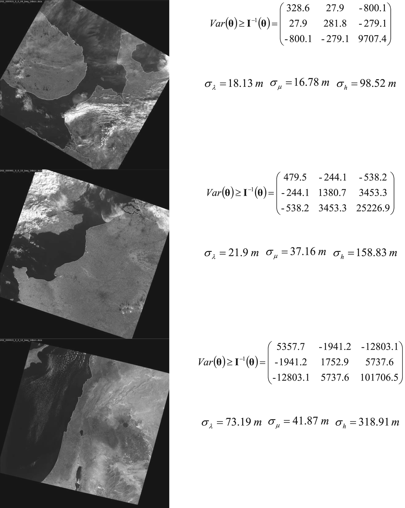
It can be seen that most of the shoreline segments in the last image are oriented in the same direction. This circumstance led to a strong correlation of latitude and longitude errors and an increase of altitude error. Error matrix calculation required less than ten milliseconds. The programme used one core and one thread of an i7-3770 Intel processor.
8. INVERSION OF FISHER INFORMATION MATRIX
The covariance matrix of the shoreline optical navigation errors is obtained by inversion of the Fisher information matrix. Unfortunately, sometimes the shape of the observed shoreline leads to bad matrix conditioning or matrix singularity. The omission of such measurements is a bad idea, however. The reason is that a shoreline with high stability and exactly known locations is rare enough and every effort to obtain navigation information must be made.
The inclusion of the inertial navigation subsystem into the navigation system and a competent solution to the problem of navigation information integration allows the utilisation of a measurement with a singular Fisher information matrix.
It is stated by Li and Yeh (Reference Li and Yeh2012) that Moore-Penrose pseudo-inversion is optimal for a singular or badly conditioned Fisher information matrix. For verification of this statement the Fisher information matrix was calculated for a straight-line artificial shoreline. The results of the calculations confirmed the conclusions of this article.
9. BIAS OF ATTITUDE ESTIMATION
It can be shown that altitude estimates from the shoreline map will have a bias. There are two ways to take this effect into account. The first way supposes the inclusion of bias into the error estimation. The second way supposes the calculation of this bias and its compensation. From the application point of view, the second way is preferable. An analysis of the methods for calculating altitude corrections will be covered in future work.
10. CONCLUSIONS
Visual shoreline navigation is one of many possible additional sources of navigation information in a GNSS-denied environment. A feature of visual shoreline navigation is the severe variability of navigation errors depending on the shape of the observed shoreline, the distance and the angle of observation. The Cramer-Rao lower bound for shoreline visual navigation errors is proposed to use as the navigation error covariance matrix. This bound is determined through errors of localisation of any shoreline segment which is used for calculating position of aircraft or spacecraft. Shoreline segment error localisation is estimated through analysis of each individual brightness profile of a border segment between ocean and land. The presented method of lower bound estimation is intended for on board real-time estimation of navigation errors for any processed cadre of information which is used for shoreline navigation.