1 Introduction
A good knowledge of the equation of state of hydrogen–helium mixtures is critical for the understanding of the formation and evolution of gas giant planets (Fortney & Nettelmann Reference Fortney and Nettelmann2010), brown dwarfs and main-sequence stars and the magnetic field generation in their deep interiors (Gastine et al. Reference Gastine, Wicht, Duarte, Heimpel and Becker2014). The warm dense matter region covering pressures up to tens of Mbar and temperatures up to a few 10 000 K is of particular interest for the interior of gas giants like Jupiter and Saturn. Fundamental processes like metallization of hydrogen and phase separation of helium from hydrogen will be reflected in the high-pressure phase diagram. However, the location of the corresponding coexistence lines is still under lively debate (McMahon et al. Reference McMahon, Morales, Pierleoni and Ceperley2012). Essential progress in this context is expected from the data of the Cassini and Juno space missions to Saturn and Jupiter, see e.g. Guillot et al. (Reference Guillot, Atreya, Charnoz, Dougherty and Read2009, Reference Guillot, Miguel, Militzer, Hubbard, Kaspi, Galanti, Cao, Helled, Wahl and Iess2018) and Hubbard et al. (Reference Hubbard, Dougherty, Gautier and Jacobson2009). New high-pressure experiments using novel diamond-anvil-cell (DAC) techniques (Dias & Silvera Reference Dias and Silvera2017), high-power optical lasers (Hicks et al. Reference Hicks, Boehly, Celliers, Eggert, Moon, Meyerhofer and Collins2009; Davis et al. Reference Davis, Döppner, Rygg, Fortmann, Divol, Pak, Fletcher, Becker, Holst and Sperling2016), pulsed power (Knudson et al. Reference Knudson, Desjarlais, Becker, Lemke, Cochrane, Savage, Bliss, Mattsson and Redmer2015; Knudson & Desjarlais Reference Knudson and Desjarlais2017) or the infrastructure at free-electron-laser (FEL) facilities such as the linac coherent light source (LCLS) (Glenzer et al. Reference Glenzer, Fletcher, Galtier, Nagler, Alonso-Mori, Barbrel, Brown, Chapman, Chen and Curry2016) will continue to improve our knowledge about matter under extreme conditions.
It has long been proposed that the helium phase separates from hydrogen under the extreme conditions in the interiors of Jupiter and Saturn (Smoluchowski Reference Smoluchowski1967; Salpeter Reference Salpeter1973), such that He-rich droplets sink deeper into the planet and thereby release gravitational energy which contributes to the intrinsic luminosity of the planet. This process might be responsible for the observed He depletion in the atmospheres of both planets (Zahn, Hunten & Lehmacher Reference Zahn, Hunten and Lehmacher1998; Conrath & Gautier Reference Conrath and Gautier2000) and the observed luminosity anomaly in Saturn (Fortney & Hubbard Reference Fortney and Hubbard2003). Standard planetary evolution models for Saturn are not able to reproduce its correct age if H–He demixing is neglected (Fortney & Hubbard Reference Fortney and Hubbard2003; Fortney et al. Reference Fortney, Ikoma, Nettelmann, Guillot and Marley2011; Püstow et al. Reference Püstow, Nettelmann, Lorenzen and Redmer2016). Only the layered convection model by Leconte & Chabrier (Reference Leconte and Chabrier2013) does not require He rain, albeit not excluding it either (see also Nettelmann et al. Reference Nettelmann, Fortney, Moore and Mankovich2015).
Experiments on the miscibility diagram at Mbar pressures have not been published so far. For lower pressures, diamond-anvil-cell experiments have been able to verify demixing at room temperature (Loubeyre, LeToullec & Pinceaux Reference Loubeyre, LeToullec and Pinceaux1991). Results from theoretical calculations have led to significantly different estimates of the high-pressure miscibility diagram (Stevenson Reference Stevenson1975; Klepeis et al.
Reference Klepeis, Schafer, Barbee and Ross1991; Pfaffenzeller, Hohl & Ballone Reference Pfaffenzeller, Hohl and Ballone1995; Lorenzen, Holst & Redmer Reference Lorenzen, Holst and Redmer2009; Morales et al.
Reference Morales, Hamel, Caspersen and Schwegler2013; Schöttler & Redmer Reference Schöttler and Redmer2018). The first ab initio calculations based on density functional theory (DFT) have been done by Klepeis et al. (Reference Klepeis, Schafer, Barbee and Ross1991) for fixed ion configurations using the local density approximation (LDA). They found a nearly pressure-independent demixing temperature of 15 000 K for the solar He concentration. Pfaffenzeller et al. (Reference Pfaffenzeller, Hohl and Ballone1995) applied Car–Parrinello molecular dynamics and demonstrated considerably lower demixing temperatures than Klepeis et al. (Reference Klepeis, Schafer, Barbee and Ross1991) and a significant pressure dependence. Lorenzen et al. (Reference Lorenzen, Holst and Redmer2009) presented the first density functional theory results coupled to Born–Oppenheimer molecular dynamics (DFT-MD) using gradient corrections for the exchange-correlation (XC) energy. They used the Perdew–Burke–Ernzerhof (PBE) XC functional (Perdew, Burke & Ernzerhof Reference Perdew, Burke and Ernzerhof1996) and applied the ideal entropy of the mixing approximation, similar to Klepeis et al. (Reference Klepeis, Schafer, Barbee and Ross1991) and Pfaffenzeller et al. (Reference Pfaffenzeller, Hohl and Ballone1995). Notably, the equation of state was calculated for 33 different He fractions in the pressure range of 4–24 Mbar and for temperatures up to 20 000 K. Later, the miscibility diagram was extended down to pressures of 1 Mbar (Lorenzen, Holst & Redmer Reference Lorenzen, Holst and Redmer2011). These results showed slightly higher demixing temperatures than those of Pfaffenzeller et al. (Reference Pfaffenzeller, Hohl and Ballone1995) and revealed a strong asymmetry in the miscibility diagram, which is caused by the melting transition of He at high helium fractions and the metallization transition in the hydrogen subsystem which requires a minimum hydrogen density of
 $n_{\text{H}}^{1/3}a_{\text{B}}\sim 0.25$
according to the Mott criterion (see Lorenzen et al.
Reference Lorenzen, Holst and Redmer2009). The approximation of ideal entropy of mixing was avoided by Morales et al. (Reference Morales, Schwegler, Ceperley, Pierleoni, Hamel and Caspersen2009, Reference Morales, Hamel, Caspersen and Schwegler2013) by calculating the non-ideal entropy of mixing using coupling-constant integration (Kirkwood Reference Kirkwood1935). This led to lower demixing temperatures compared to the ideal entropy case and altered the low-pressure and low-temperature behaviour. The extensive DFT-MD data of Lorenzen et al. (Reference Lorenzen, Holst and Redmer2009, Reference Lorenzen, Holst and Redmer2011) were used to calculate the inhomogeneous planetary evolution of Saturn (Püstow et al.
Reference Püstow, Nettelmann, Lorenzen and Redmer2016). It was shown that the Lorenzen miscibility diagram slows the cooling of Saturn significantly, but leads to a too large cooling time. Better agreement with the age of the solar system could be obtained when the demixing temperatures of the Lorenzen miscibility diagram were lowered by 1300 K to be more in agreement with the data by Morales et al. (Reference Morales, Hamel, Caspersen and Schwegler2013).
The equation of state (EOS) is of major importance when calculating planetary models and their evolution. It was shown that different equations of state can have a significant impact on model predictions (Miguel, Guillot & Fayon Reference Miguel, Guillot and Fayon2016; Wahl et al. Reference Wahl, Hubbard, Militzer, Guillot, Miguel, Movshovitz, Kaspi, Helled, Reese and Galanti2017), especially on the allowed abundance of heavier elements. Commonly used wide-range equations of state are those of Becker et al. (Reference Becker, Lorenzen, Fortney, Nettelmann, Schoettler and Redmer2014) (REOS.3) and Saumon, Chabrier & van Horn (Reference Saumon, Chabrier and van Horn1995) (SCvH) which are available for pure hydrogen and pure helium. The SCvH EOS is based on a single model for the free energy while the H/He-REOS.3 uses a combination of different free energy models and DFT-MD to improve the highly correlated warm dense matter regime. The EOS of a H–He mixture is then available using the linear mixing approximation (Bethkenhagen et al. Reference Bethkenhagen, Meyer, Hamel, Nettelmann, French, Scheibe, Ticknor, Collins, Kress and Fortney2017). This approximation can only be avoided if the EOS is calculated for specific mixing ratios as done by Militzer (Reference Militzer2013) for near solar composition.
The PBE XC functional has been used in the DFT-MD calculations of Becker et al., Lorenzen et al., Militzer et al. and Morales et al. However, recent experiments on the metallization transition of liquid deuterium (Knudson et al. Reference Knudson, Desjarlais, Becker, Lemke, Cochrane, Savage, Bliss, Mattsson and Redmer2015; Ohta et al. Reference Ohta, Ichimaru, Einaga, Kawaguchi, Shimizu, Matsuoka, Hirao and Ohishi2015; Zaghoo, Salamat & Silvera Reference Zaghoo, Salamat and Silvera2016) and the deuterium Hugoniot (Knudson & Desjarlais Reference Knudson and Desjarlais2017) gave contradicting results regarding the metallization pressure and thus the accuracy of PBE. In general, DFT results obtained with various functionals show H metallization pressures which deviate by up to 1.5 Mbar (Knudson et al. Reference Knudson, Desjarlais, Becker, Lemke, Cochrane, Savage, Bliss, Mattsson and Redmer2015; Knudson & Desjarlais Reference Knudson and Desjarlais2017). The PBE functional supports the experiments by Ohta et al. (Reference Ohta, Ichimaru, Einaga, Kawaguchi, Shimizu, Matsuoka, Hirao and Ohishi2015) and Zaghoo et al. (Reference Zaghoo, Salamat and Silvera2016), but the van der Waals density functional (vdW-DF) of Dion et al. (Reference Dion, Rydberg, Schröder, Langreth and Lundqvist2004) supports the experiments by Knudson et al. (Reference Knudson, Desjarlais, Becker, Lemke, Cochrane, Savage, Bliss, Mattsson and Redmer2015). However, high-precision Hugoniot data are not reproduced perfectly by any functional (Knudson & Desjarlais Reference Knudson and Desjarlais2017). Quantum Monte Carlo (QMC) simulations of Mazzola, Helled & Sorella (Reference Mazzola, Helled and Sorella2018) have reproduced the experiments by Ohta et al. (Reference Ohta, Ichimaru, Einaga, Kawaguchi, Shimizu, Matsuoka, Hirao and Ohishi2015) and Zaghoo et al. (Reference Zaghoo, Salamat and Silvera2016) while the QMC calculations of Tubman et al. (Reference Tubman, Liberatore, Pierleoni, Holzmann and Ceperley2015) fail to reproduce the deuterium Hugoniot (Knudson & Desjarlais Reference Knudson and Desjarlais2017). Similarly, the PBE and vdW-DF do not agree perfectly with the high-precision Hugoniot data. Due to these discrepancies in theoretical and experimental results, there is currently no final answer to the location of the metallization transition and the correct choice of the XC functional for hydrogen. For helium, the available experimental data are not accurate enough to discriminate different XC functionals (Preising et al. Reference Preising, Lorenzen, Becker, Redmer, Knudson and Desjarlais2018).
Still, benchmarking studies of several XC functionals with QMC calculations have shown that the vdW-DF overestimates the pressure in hydrogen–helium mixtures but shows best performance for the enthalpy (Clay III et al. Reference Clay, Holzmann, Ceperley and Morales2016). The enthalpy is of major importance when calculating phase equilibria. Thus, if the miscibility of H–He mixtures is of interest, the vdW-DF should be used. Recently, the miscibility diagram of hydrogen–helium mixtures has been calculated using the vdW-DF (Schöttler & Redmer Reference Schöttler and Redmer2018). Here, we will present additional results related to the miscibility diagram and demonstrate how the non-ideal entropy can be obtained using different methods. We will also present our equation of state data for the vdW-DF and show the free enthalpy of mixing of hydrogen–helium mixtures. The influence of nuclear quantum corrections (NQC) will be discussed.
2 Methods
2.1 Density functional theory
We performed finite-temperature density functional theory simulations which were coupled to classical molecular dynamics for the ions (FT-DFT-MD). The plane-wave code VASP (Kresse & Hafner Reference Kresse and Hafner1993; Kresse & Furthmüller Reference Kresse and Furthmüller1996a
,Reference Kresse and Furthmüller
b
; Klimeš, Bowler & Michaelides Reference Klimeš, Bowler and Michaelides2010, Reference Klimeš, Bowler and Michaelides2011) was used. Simulations were done with the non-local van der Waals density functional of Dion et al. (vdW-DF) (Dion et al.
Reference Dion, Rydberg, Schröder, Langreth and Lundqvist2004). Simulations in the NVT ensemble were performed for constant electron numbers of 64 for the miscibility calculations and 256 for isentropes and entropies. The Nose–Hoover thermostat (Hoover Reference Hoover1985) was used to ensure a canonical ensemble. A plane-wave cutoff of 1200 eV and the Baldereschi mean-value (Baldereschi Reference Baldereschi1973)
 $\boldsymbol{k}$
point was used to obtain energies
 $u$
and pressures
 $p$
that were converged to within 1 %. Averages of
 $p$
and
 $u$
were taken for at least 10 000 time steps (2 ps) after thermodynamic equilibrium was reached. For the smaller electron number we performed simulations for 31 different He concentrations in the pressure range from 0.2 to 30 Mbar and temperatures every 1000 K in the range of 1000–15 000 K. Convergence with respect to electron number was checked for pure H and He and one mixture, where a maximum deviation of 1 % in pressure and energy was seen between simulations with 64 and 256 electrons. Additionally, a mixture with 220 H and 18 He atoms was simulated using the vdW-DF on which the isentropes in figure 8(b) are based. This mixture was used by Hubbard & Militzer (Reference Hubbard and Militzer2016) to calculate a preliminary Jupiter model. The obtained EOS data were corrected for nuclear quantum effects by applying the correction formulas given by Berens et al. (Reference Berens, Mackay, White and Wilson1983).
2.2 Entropy calculations
2.2.1 Thermodynamic integration
The entropy for arbitrary densities and temperatures can be calculated via thermodynamic integration (TI) over the equation of state: If pressure
 $p$
and temperature
 $T$
are used as independent variables, the entropy
 $S$
can be written as
 $$\begin{eqnarray}\displaystyle S(p,T) & = & \displaystyle \frac{U(p,T)+pV(p,T)}{T}-\int _{p_{0}}^{p}\,\text{d}p^{\prime }\frac{V(p^{\prime },T_{0})}{T_{0}}\nonumber\\ \displaystyle & & \displaystyle +\,\int _{T_{0}}^{T}\,\text{d}T^{\prime }\frac{U(p,T^{\prime })+pV(p,T^{\prime })}{T^{\prime 2}}-\frac{G_{0}}{T_{0}},\end{eqnarray}$$
where
 $G_{0}=U(p_{0},T_{0})+p_{0}V(p_{0},T_{0})-T_{0}S(p_{0},T_{0})$
is a constant that includes the unknown absolute entropy at the reference point
 $(p_{0},T_{0})$
. In principle, it is possible to use the entropy in the ideal gas limit as a reference, but the required equation of state data in this limit cannot be obtained via DFT-MD simulations because of drastically increasing computational costs for low densities. Thus, one would need to construct a wide-range EOS from different EOS models as done by Becker et al. (Reference Becker, Lorenzen, Fortney, Nettelmann, Schoettler and Redmer2014). To avoid this huge effort for 31 different He concentrations, we tested alternative approaches which are explained in the following sections.
2.2.2 Coupling-constant integration
Coupling-constant integration (CCI)Footnote
1
(Kirkwood Reference Kirkwood1935) is a method to calculate the change in free energy when the potential energy is adiabatically switched from one system with potential
 $U_{0}$
to another potential
 $U_{1}$
. The parameter denoting the coupling strength is usually called the coupling constant
 $\unicode[STIX]{x1D706}$
. The systems
 $U_{0}$
and
 $U_{1}$
can be linearly combined such that
 $$\begin{eqnarray}U(\unicode[STIX]{x1D706})=(1-\unicode[STIX]{x1D706})U_{0}+\unicode[STIX]{x1D706}U_{1}.\end{eqnarray}$$
The difference in free energy
 $\unicode[STIX]{x0394}F$
is then
 $$\begin{eqnarray}\displaystyle \unicode[STIX]{x0394}F & = & \displaystyle \int _{0}^{1}\left\langle \frac{\unicode[STIX]{x2202}U(\unicode[STIX]{x1D706})}{\unicode[STIX]{x2202}\unicode[STIX]{x1D706}}\right\rangle _{\unicode[STIX]{x1D706}}\,\text{d}\unicode[STIX]{x1D706},\end{eqnarray}$$
 $$\begin{eqnarray}\displaystyle & = & \displaystyle \int _{0}^{1}\langle U_{1}-U_{0}\rangle _{\unicode[STIX]{x1D706}}\,\text{d}\unicode[STIX]{x1D706}.\end{eqnarray}$$
The ensemble average denotes that the system is simulated using the potential
 $U(\unicode[STIX]{x1D706})$
at the given
 $\unicode[STIX]{x1D706}$
value. To perform the integration, many simulations with different
 $\unicode[STIX]{x1D706}$
values have to be done, which is the main reason why CCI is in general too demanding to be performed for every EOS point. The free energy of a reference system must be known to obtain the absolute free energy of the system of interest. While the free energy of the ideal gas
 $F_{\text{id}}$
is known in principle, it is numerically not feasible to use it as the reference system for the integration towards the DFT system. Instead an intermediate integration towards a classical force field is introduced such that the total free energy
 $F_{\text{DFT}}$
of the DFT system can be written as
 $$\begin{eqnarray}F_{\text{DFT}}=F_{\text{id}}+\unicode[STIX]{x0394}F_{\text{id}\rightarrow \text{cl}}+\unicode[STIX]{x0394}F_{\text{cl}\rightarrow \text{DFT}},\end{eqnarray}$$
where
 $\unicode[STIX]{x0394}F_{\text{id}\rightarrow \text{cl}}$
is the free energy difference of the classical force field to the ideal gas (which can be easily obtained using Monte Carlo simulations) and
 $\unicode[STIX]{x0394}F_{\text{cl}\rightarrow \text{DFT}}$
is the free energy difference of the DFT system to the force field. Militzer (Reference Militzer2013) has shown that in finite-temperature DFT calculations that the corresponding energy in (2.4) should be replaced with the Mermin free energy
 $\unicode[STIX]{x1D6FA}_{\text{DFT}}=U_{\text{DFT}}-TS_{\text{el}}$
, because the forces are derived from this quantity which incorporates the ideal electronic entropy via
 $S_{\text{el}}$
. At higher temperatures, the electronic entropy cannot be neglected. The total entropy
 $S$
is then given by
 $$\begin{eqnarray}S=\frac{U_{\text{DFT}}-F_{\text{DFT}}}{T}.\end{eqnarray}$$
To accelerate the calculations it is mandatory that the classical potential resembles the energy and radial pair distribution function (RDF) of the DFT system. The number of
 $\unicode[STIX]{x1D706}$
values can be decreased significantly if a good model can be found. In our work, we used the reflected Yukawa-type pair potentials given by Morales et al. (Reference Morales, Schwegler, Ceperley, Pierleoni, Hamel and Caspersen2009):
 $$\begin{eqnarray}U(r)=\left\{\begin{array}{@{}ll@{}}a\left({\displaystyle \frac{\text{e}^{-br}}{r}}+{\displaystyle \frac{\text{e}^{-b(L-r)}}{L-r}}-4{\displaystyle \frac{\text{e}^{-bL/2}}{L}}\right)\quad & r\leqslant L/2,\\ 0\quad & r>L/2,\end{array}\right.\end{eqnarray}$$
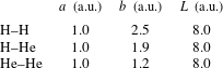
where the coefficients
 $a$
,
 $b$
and
 $L$
are given in table 1. In contrast to Morales et al. (Reference Morales, Schwegler, Ceperley, Pierleoni, Hamel and Caspersen2009), we chose the reference point to be at
 $T=10\,000$
K and a Wigner–Seitz radius of
 $r_{s}=1.4~\text{a}_{0}$
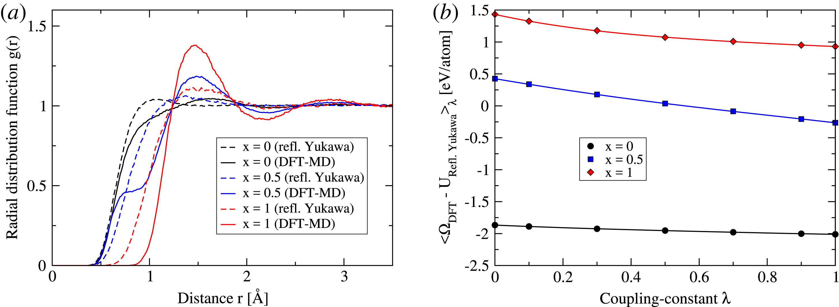
, i.e. slightly lower densities. These parameters ensure that no demixing occurs inside the simulation box for all considered He fractions. In figure 1(a) the total RDF of the reflected Yukawa potential and the DFT-MD are shown for H, He and a mixture. It is obvious that the potentials do not offer a perfect resemblance to the DFT system. For pure hydrogen the minimal distance in the RDF is reproduced but the subsequent structure at higher distances is missed. For pure helium the onset of the RDF is not reproduced by the reflected Yukawa potential but the position of the first maximum at 1.5 Å is captured. Despite the differences in the RDF, the integrand in (2.4) shows smooth curves in figure 1(b) and the integration can be performed using fourth-order polynomial fits to the data.
(a) Radial pair distribution function for the reflected Yukawa potential (
 $\unicode[STIX]{x1D706}=0$
) and DFT-MD system (
 $\unicode[STIX]{x1D706}=1$
) at the reference point
 $T=10\,000$
K and
 $r_{s}=1.4~\text{a}_{0}$
. (b) Integrand of (2.4) for the same conditions, where
 $U_{\text{DFT}}$
has been replaced by
 $\unicode[STIX]{x1D6FA}_{\text{DFT}}=U_{\text{DFT}}-TS_{\text{el}}$
(see text). Lines are polynomial fits of fourth order.

Coefficients for the reflected Yukawa pair potentials (Morales et al. Reference Morales, Schwegler, Ceperley, Pierleoni, Hamel and Caspersen2009). Values are given in atomic units.

2.2.3 Reduced coupling-constant integration
One particular drawback of the CCI approach (despite the required classical potential) is the need for simulations at many different
 $\unicode[STIX]{x1D706}$
values. We found that seven values are sufficient to obtain well-converged free energies. Still, it would be beneficial to further lower the number of coupling constants. For this, one considers a series expansion of the integrand in (2.3) centred around
 $\unicode[STIX]{x1D706}_{0}$
(Smith & Gunsteren Reference Smith and Gunsteren1994; Hummer & Szabo Reference Hummer and Szabo1996). Truncating this series after the linear term yields:
 $$\begin{eqnarray}\unicode[STIX]{x0394}F\simeq \langle U_{1}-U_{0}\rangle _{\unicode[STIX]{x1D706}_{0}}-\frac{1-2\unicode[STIX]{x1D706}_{0}}{2k_{\text{B}}T}\{\langle (U_{1}-U_{0})^{2}\rangle _{\unicode[STIX]{x1D706}_{0}}-\langle U_{1}-U_{0}\rangle _{\unicode[STIX]{x1D706}_{0}}^{2}\}.\end{eqnarray}$$
This reduced coupling-constant integration (RCCI) allows for the approximate evaluation of
 $\unicode[STIX]{x0394}F$
using only one coupling constant
 $\unicode[STIX]{x1D706}_{0}$
. In general, this approach is only valid if the classical system reproduces the structure and energetics of the DFT-MD system with high accuracy. However, we will show in § 2.2.5, that accurate results for the total entropy and entropy of mixing of H–He mixtures can be obtained even with the reflected Yukawa potential, that shows no perfect resemblance to the DFT-MD system, cf. figure 1.
2.2.4 The 2-phase thermodynamic memory-function method
The calculation of ionic entropies for liquids is possible by integrating the vibrational density of states (VDOS) using an appropriate weighting function (Lin, Blanco & Goddard III Reference Lin, Blanco and Goddard2003; Lin, Maiti & Goddard III Reference Lin, Maiti and Goddard2010; Lai, Hsieh & Lin Reference Lai, Hsieh and Lin2012; Desjarlais Reference Desjarlais2013; Meyer et al.
Reference Meyer, Ticknor, Kress and Collins2016). The VDOS has to be separated into a gas-like and a solid-like component, where the solid part is described with the weighting function of a harmonic oscillator and the gas part with the hard-sphere model (Lin et al.
Reference Lin, Blanco and Goddard2003). This so-called 2-phase thermodynamic (2PT) method has been modified by Desjarlais (Reference Desjarlais2013) who described the gas-like part using a memory-function ansatz (2PT-MF method), which improved the accuracy for liquid metals to 1 %. An extension of the 2PT method to multi-component systems has been given by Lai et al. (Reference Lai, Hsieh and Lin2012), and is also applicable to the 2PT-MF method (see French, Desjarlais & Redmer Reference French, Desjarlais and Redmer2016). The application to multicomponent systems requires knowledge about the partial volumes
 $\unicode[STIX]{x1D709}_{i}=V_{i}/N_{i}$
of all constituents
 $i$
for all temperatures and pressures considered (cf. equations (8) and (11) of French et al.
Reference French, Desjarlais and Redmer2016). Obtaining the partial volumes is in general quite demanding and requires additional simulations with varying particle numbers. For our H–He data however, we were able to calculate the partial volumes using the method of intercepts with no additional costs, see § 2.3.2 for details. The advantage of the 2PT-MF method is that entropies can be computed from a single molecular dynamics run without the need for classical pair potentials and additional demanding simulations as in the CCI approach.
2.2.5 Comparison of the entropy methods
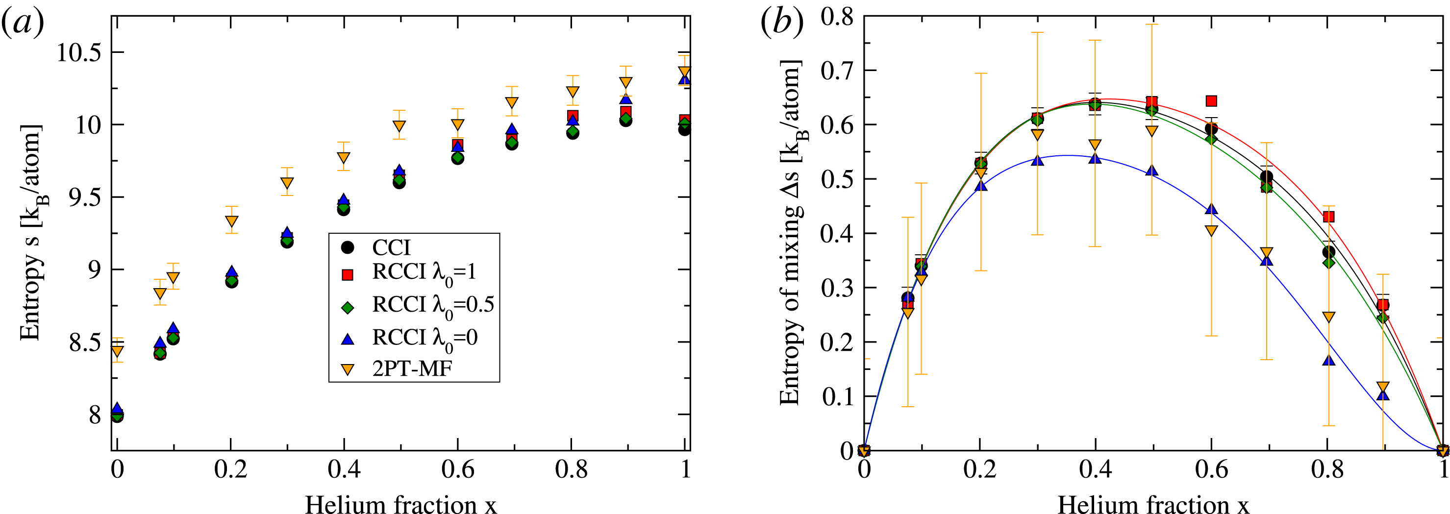
Entropy (a) and entropy of mixing (b) of H–He mixtures as a function of He fraction
 $x$
at
 $T=10\,000$
K and
 $r_{\text{s}}=1.4~\text{a}_{0}$
. Data for the coupling-constant integration (CCI), reduced coupling-constant integration (RCCI) and 2PT-MF method (see Desjarlais Reference Desjarlais2013) have been obtained using the vdW-DF.

In figure 2 we show the total entropy and the corresponding entropy of mixing for various He fractions. We calculated the entropy using the full CCI approach, the RCCI approach for three
 $\unicode[STIX]{x1D706}_{0}$
values and the 2PT-MF method. The CCI method is most accurate with an estimated error of
 $0.01~k_{\text{B}}/\text{atom}$
. An error of 1 % is shown for the 2PT-MF method, yet it overestimates the CCI entropies significantly. While the 2PT-MF method works well for liquid metals near the melting line (Desjarlais Reference Desjarlais2013), we observe deviations of up to
 $0.46~k_{\text{B}}/\text{atom}$
compared to the CCI approach. For the entropy of mixing (figure 2
b) an estimated uncertainty of 1 % in the 2PT-MF entropies yields an error of
 ${\sim}0.2~k_{\text{B}}/\text{atom}$
, which translates into a relative error of at least 30 %. Unfortunately, this renders the 2PT-MF method inapplicable for H–He mixtures. The RCCI shows in general a much smaller deviation to the full CCI approach than the 2PT-MF method. For a value of
 $\unicode[STIX]{x1D706}_{0}=0$
the deviation is largest on average with a maximum error of
 $0.34~k_{\text{B}}/\text{atom}$
at
 $x=1$
. For
 $\unicode[STIX]{x1D706}_{0}=1$
the agreement with CCI is better with a maximum error of
 $0.12~k_{\text{B}}/\text{atom}$
at
 $x=0.8$
. Best performance of the RCCI method could be achieved for a value of
 $\unicode[STIX]{x1D706}_{0}=0.5$
where a maximum error of
 $0.042~k_{\text{B}}/\text{atom}$
can be seen at
 $x=1$
. These results are quite interesting given the performance of the reflected Yukawa potential at these conditions, cf. figure 1(a). On the one hand, our calculations show, that even less accurate potentials can yield high accuracy entropies with the CCI method, on the other hand, they show that the computational effort can be decreased significantly if special attention is paid to finding a good pair potential. More importantly, if
 $\unicode[STIX]{x1D706}_{0}=1$
is chosen, the RCCI method can be applied without modifications in the DFT-MD code, because the simulation is performed with pure DFT forces and the classical potential can be evaluated on the DFT-MD trajectory in a post-processing step to evaluate the ensemble averages of (2.8). Still, in our work we decided to use the CCI method for calculating the reference entropies for the TI via the equation of state, (2.1).
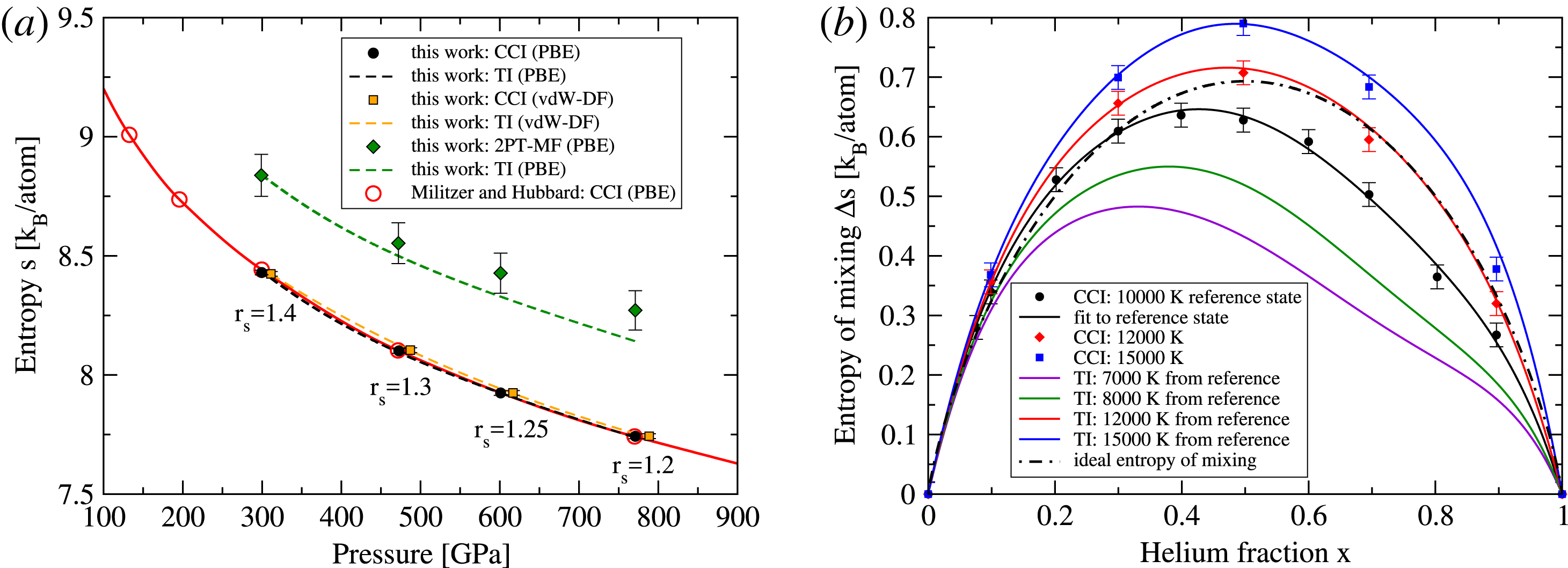
(a) Entropy at 10 000 K for a H–He mixture with
 $x=0.0756$
as a function of pressure. The CCI entropy for four different densities using the PBE functional (black circles) and the vdW-DF (orange squares) is shown. The 2PT-MF entropy has been evaluated for the PBE functional. PBE and vdW-DF calculations have been performed for four Wigner–Seitz radii
 $r_{\text{s}}$
given in atomic units. Dashed lines are obtained using (2.1), where the constant
 $G_{0}$
was determined from the entropy value at
 $r_{\text{s}}=1.4~\text{a}_{0}$
for the corresponding method. The black and green TI curves for PBE are thus only shifted by a constant. Red open circles are from Militzer & Hubbard (Reference Militzer and Hubbard2013). (b) Entropy of mixing for five temperatures at a Wigner–Seitz radius of
 $r_{\text{s}}=1.4~\text{a}_{0}$
. Symbols are CCI calculations. Black solid line is a Redlich–Kister (RK) fit of fourth order of the CCI data. Coloured solid lines are obtained using TI, (2.1), where the reference entropy is the RK fit of the 10 000 K CCI data.

In figure 3 we show the performance of the TI method. Figure 3(a) shows the entropy as a function of pressure at a temperature of 10 000 K for a H–He mixture with
 $x=0.0756$
. We computed the CCI entropies for the four shown Wigner–Seitz radii. Results using the PBE functional agree with the calculations by Militzer & Hubbard (Reference Militzer and Hubbard2013). The 2PT-MF method calculated for the PBE functional overestimates the entropy significantly, as shown in figure 2(a). The dashed lines are TI results using (2.1). We chose the reference entropy that determines the constant
 $G_{0}$
to be the entropy value at
 $r_{\text{s}}=1.4~\text{a}_{0}$
given by the respective method (CCI, 2PT-MF) and functional (PBE, vdW-DF). The TI curves agree perfectly with the CCI results for the PBE functional and the vdW-DF. The 2PT-MF method, despite overestimating the entropy significantly, yields entropies that do not reproduce the thermodynamic integration via the equation of state and therefore are not thermodynamically consistent. Figure 3(b) shows the entropy of mixing for the vdW-DF as function of
 $x$
for different
 $T$
at a constant Wigner–Seitz radius of
 $r_{\text{s}}=1.4~\text{a}_{0}$
. Symbols are CCI calculations. The black solid line is a Redlich–Kister (RK) fit (Redlich & Kister Reference Redlich and Kister1948) of fourth order of the 10 000 K data, see (2.13). The other coloured lines have been obtained using TI where the reference entropy for every He fraction is the RK fit of the 10 000 K CCI data. For 12 000 K and 15 000 K the CCI entropies agree with TI within the given error bars except for 15 000 K at
 $x=0.9$
where the TI yields slightly higher entropies. Nevertheless, the thermodynamic integration via the equation of state is well suited to obtaining entropies at arbitrary pressures and temperatures.
2.3 Thermodynamics of binary mixtures
2.3.1 Free enthalpy of mixing
The central quantity for miscibility calculations is the free enthalpy of mixing:
 $$\begin{eqnarray}\unicode[STIX]{x0394}G(x,p,T)=G(x,p,T)-xG(1,p,T)-(1-x)G(0,p,T),\end{eqnarray}$$
where
 $G$
is the free enthalpy as a function of helium number fraction
 $x$
, pressure
 $p$
and temperature
 $T$
. The enthalpy for pure H (
 $x=0$
), pure He (
 $x=1$
) and mixtures of both is given by
 $$\begin{eqnarray}G(x,p,T)=U(x,p,T)-TS(x,p,T)+pV(x,p,T),\end{eqnarray}$$
where
 $U$
is the internal energy,
 $V$
is the volume and
 $S$
the entropy. A binary mixture is thermodynamically unstable if
 $$\begin{eqnarray}\frac{\unicode[STIX]{x2202}^{2}\unicode[STIX]{x0394}G(x,p,T)}{\unicode[STIX]{x2202}x^{2}}<0,\end{eqnarray}$$
i.e. a system with
 $x$
inside the unstable region decomposes into two subsystems with different helium fractions
 $x_{1}$
and
 $x_{2}$
given by the inflection points. The ensemble of He fractions determined by this criterion is called the spinodal curve. However, there are He fractions outside the spinodal region, where the coexisting phases are not in thermodynamic equilibrium. This is only achieved when the chemical potentials in both phases are equal, i.e. when a common tangent can be applied to the Gibbs free energy of mixing, so that the slope at the He fraction of the He-poor phase
 $x_{1}$
is equal to the slope at the He fraction of the He-rich phase
 $x_{2}$
, i.e.:
 $$\begin{eqnarray}\frac{\unicode[STIX]{x0394}G(x_{2},p,T)-\unicode[STIX]{x0394}G(x_{1},p,T)}{x_{2}-x_{1}}=\left.\frac{\unicode[STIX]{x2202}\unicode[STIX]{x0394}G(x,p,T)}{\unicode[STIX]{x2202}x}\right|_{x_{1}}=\left.\frac{\unicode[STIX]{x2202}\unicode[STIX]{x0394}G(x,p,T)}{\unicode[STIX]{x2202}x}\right|_{x_{2}}.\end{eqnarray}$$
These two points mark the so-called binodal region. The time scales on which thermodynamic equilibrium is reached are much shorter than the time scales on which planetary evolution takes place so that the binodal region has to be considered for planetary applications. Numerically, the common tangent construction is applied by fitting the discrete free enthalpy of mixing for fixed pressure and temperature to a RK expansion (Redlich & Kister Reference Redlich and Kister1948):
 $$\begin{eqnarray}\unicode[STIX]{x0394}G^{\text{RK}}(x)=(x^{2}-x)\left[\mathop{\sum }_{i=0}^{l}A_{i}(2x-1)^{i}\right],\end{eqnarray}$$
where
 $l$
is the degree of the polynomial.
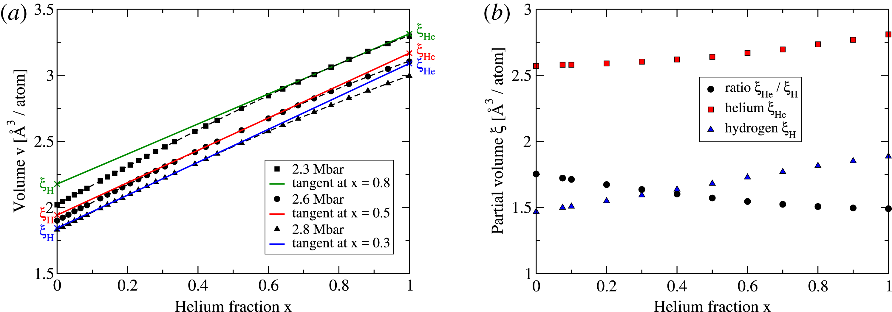
(a) Volume versus He fraction for three pressures at 10 000 K. The determination of partial volumes for H and He is demonstrated for three He fractions corresponding to the data of figure 2. Partial volumes are indicated by the crosses. (b) Partial volumes and their ratio at
 $T=10\,000$
K and
 $r_{\text{s}}=1.4~\text{a}_{0}$
for all considered He fractions.

2.3.2 Partial volume
The partial volume
 $\unicode[STIX]{x1D709}_{\unicode[STIX]{x1D6FC}}$
is defined as
 $$\begin{eqnarray}\unicode[STIX]{x1D709}_{\unicode[STIX]{x1D6FC}}=\left(\frac{\unicode[STIX]{x2202}V}{\unicode[STIX]{x2202}N_{\unicode[STIX]{x1D6FC}}}\right)_{p,T,\{N_{\unicode[STIX]{x1D6FD}\neq \unicode[STIX]{x1D6FC}}\}},\end{eqnarray}$$
with
 $V$
being the volume and
 $N_{\unicode[STIX]{x1D6FC}}$
being the particle number of species
 $\unicode[STIX]{x1D6FC}$
. Evaluating this equation numerically by inserting and removing particles to the simulation box at constant pressure and temperature is in principle possible but quite demanding. Alternatively, we can calculate the partial volumes from our extensive H–He EOS data by applying the method of intercepts (Earl Reference Earl1989). For a binary system the specific volume
 $v=V/N$
can be written as
 $$\begin{eqnarray}v(x,p,T)=(1-x)\unicode[STIX]{x1D709}_{1}(x,p,T)+x\unicode[STIX]{x1D709}_{2}(x,p,T).\end{eqnarray}$$
It can be shown that the derivative with respect to
 $x$
at constant
 $p$
and
 $T$
evaluated at
 $x^{\prime }$
is
 $$\begin{eqnarray}\left.\left(\frac{\unicode[STIX]{x2202}v(x,p,T)}{\unicode[STIX]{x2202}x}\right)_{p,T}\right|_{x=x^{\prime }}=\unicode[STIX]{x1D709}_{2}(x^{\prime })-\unicode[STIX]{x1D709}_{1}(x^{\prime }).\end{eqnarray}$$
The tangent
 $t(x)$
, that can be applied to
 $v(x)$
at
 $x^{\prime }$
has the form
 $$\begin{eqnarray}t(x)=[\unicode[STIX]{x1D709}_{2}(x^{\prime })-\unicode[STIX]{x1D709}_{1}(x^{\prime })](x-x^{\prime })+v(x^{\prime }).\end{eqnarray}$$
Inserting (2.15) at
 $x=x^{\prime }$
into the tangent equation one arrives at
 $$\begin{eqnarray}t(x)=\unicode[STIX]{x1D709}_{1}(x^{\prime })+[\unicode[STIX]{x1D709}_{2}(x^{\prime })-\unicode[STIX]{x1D709}_{1}(x^{\prime })]x.\end{eqnarray}$$
Thus, the tangent to
 $v(x)$
at
 $x=x^{\prime }$
yields the partial volume
 $\unicode[STIX]{x1D709}_{1}$
at
 $x=0$
and
 $\unicode[STIX]{x1D709}_{2}$
at
 $x=1$
. This method is illustrated in figure 4(a) for three pressures at a constant temperature of 10 000 K. The tangents at the given pressures and He fractions correspond to conditions of figure 2, i.e. a constant Wigner–Seitz radius of
 $r_{\text{s}}=1.4~\text{a}_{0}$
. In figure 4(b) the partial volumes and their ratio are shown for all He fractions. The partial volumes vary only weakly with He fraction for the given conditions, but the resulting influence on the 2PT-MF entropies is of the order of
 $0.01~k_{\text{B}}/\text{atom}$
and cannot be neglected.
3 Results
3.1 Equation of state
The discrete simulation data (energy
 $u$
and pressure
 $p$
as a function of volume
 $v$
, temperature
 $T$
and helium fraction
 $x$
) are inverted such that energy and volume are given as functions of
 $p$
,
 $T$
and
 $x$
. We fit
 $u(p)$
and
 $v(p)$
at constant
 $T$
and
 $x$
using the following functions:
 $$\begin{eqnarray}\displaystyle & \displaystyle \ln v(p)=\mathop{\sum }_{i=0}^{4}A_{i}(\ln p)^{i}, & \displaystyle\end{eqnarray}$$
 $$\begin{eqnarray}\displaystyle & \displaystyle \ln (u(p)+c)=\mathop{\sum }_{i=0}^{4}B_{i}(\ln p)^{i}, & \displaystyle\end{eqnarray}$$
where
 $A_{i}$
and
 $B_{i}$
are coefficients and
 $c=10$
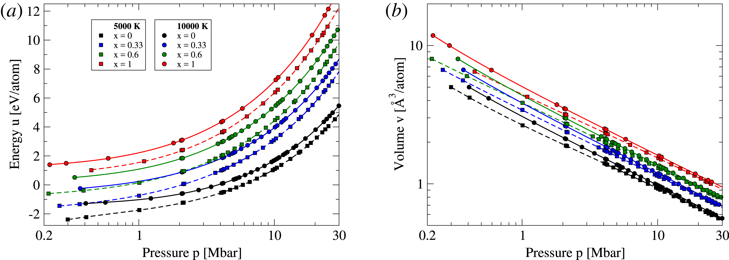
is a constant that shifts the energy to positive values avoiding complex logarithms. In figure 5 the equation of state is shown for two temperatures and four He fractions (without NQC). Fits obtained with (3.1) and (3.2) are shown as lines. Both energy and volume are fitted very well using the given fit functions. In principle it would be desirable to obtain a two-dimensional fit of both
 $p$
and
 $T$
but all tested model functions had an inferior accuracy compared to the one-dimensional fit.
(a) Energy as a function of pressure for two temperatures and four He fractions. (b) Volume as function of pressure for the same conditions as (a). Solid and dashed lines are fits.

3.2 Free enthalpy of mixing
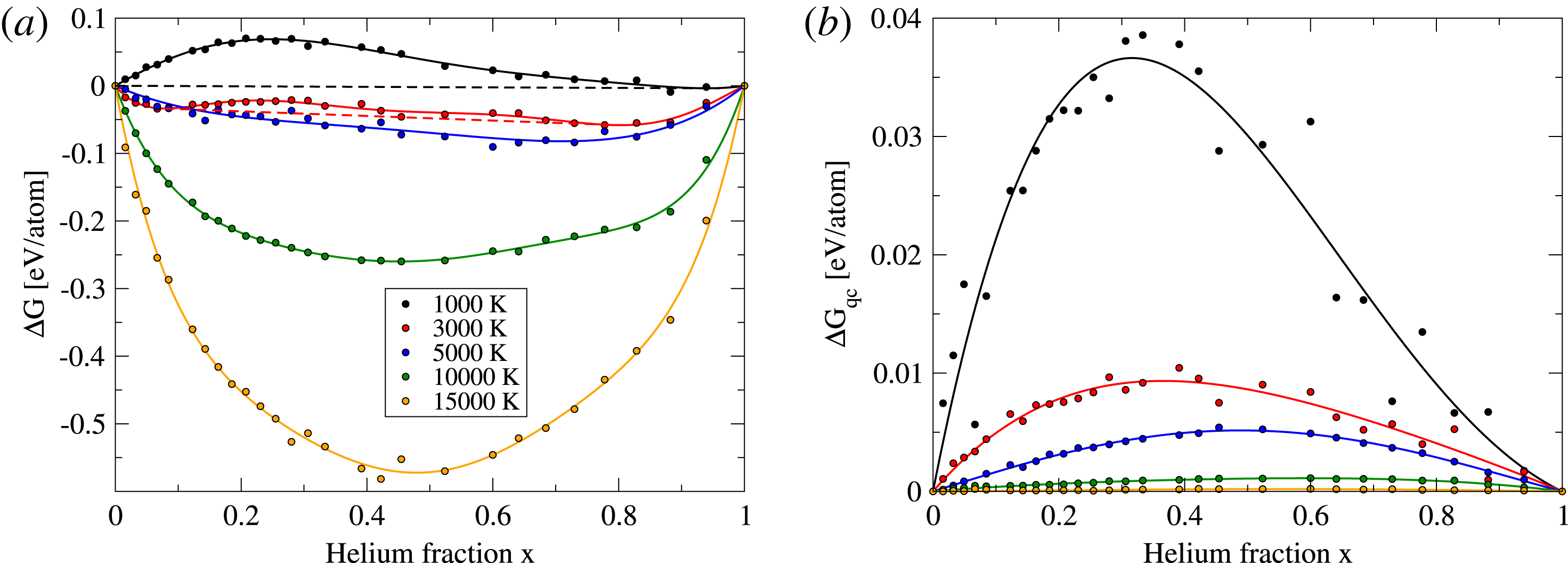
(a) Total free enthalpy of mixing (including quantum corrections) at 1 Mbar for various temperatures (colour coded). Solid lines are Redlich–Kister fits of fifth order and straight dashed lines show the double tangent construction to
 $\unicode[STIX]{x0394}G$
where it applies. (b) Quantum corrections to the free enthalpy of mixing. Colour code is the same as in (a).

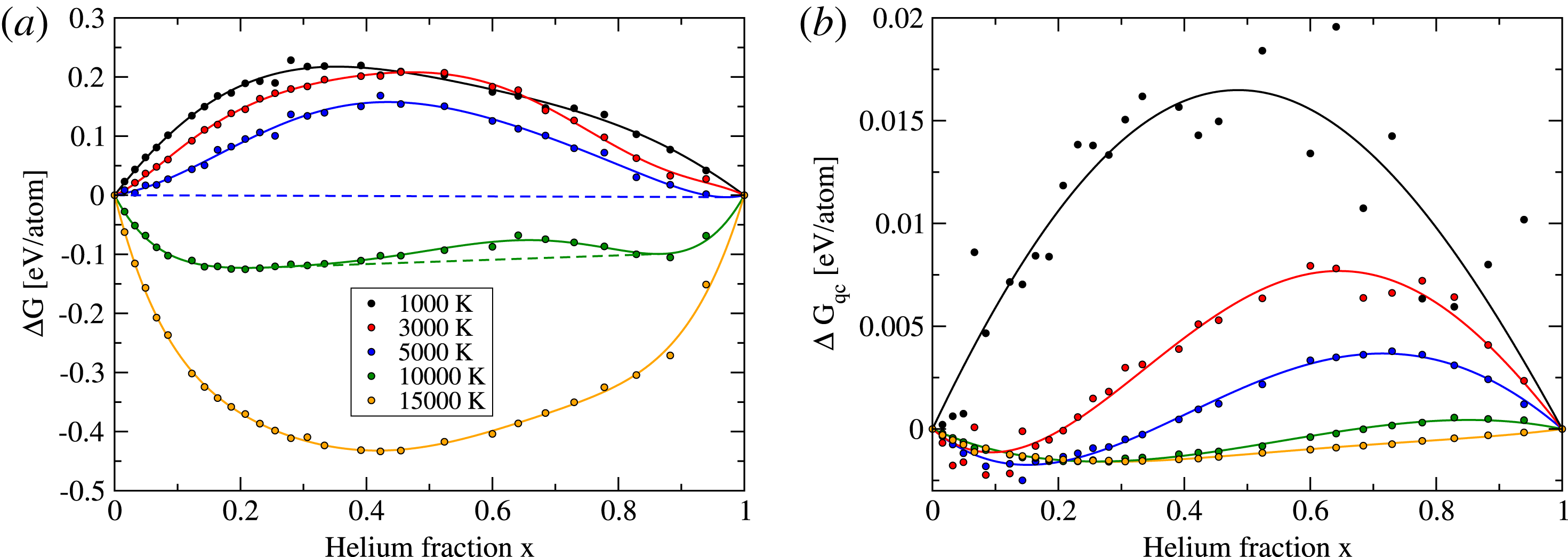
The free enthalpy of mixing has been calculated using the FT-DFT-MD data and the entropies obtained via CCI and TI. Nuclear quantum corrections (NQC) have been added. In both figures 6 and 7 the total free enthalpy of mixing (a) and the NQC to the free enthalpy (b) are shown for five temperatures and a pressure of 1 Mbar and 10 Mbar, respectively. Redlich–Kister fits of fifth order have been applied to the total free enthalpy of mixing. Dashed straight lines show the double tangent construction, where it can be applied. At 1 Mbar (figure 6), the free enthalpy of mixing shows demixing for temperatures up to 3000 K. In this temperature and pressure range, the NQC contribute significantly to the total free enthalpy and enhance the insolubility. Without quantum effects, there would be no demixing at 3000 K. For higher temperatures, the NQC still tend to favour complete demixing, but are already small enough that no demixing can be seen in the total free enthalpy. At 10 Mbar (figure 7), demixing is present up to temperatures of 11 000 K (10 000 K is the highest shown temperature in the figure, where demixing occurs). The contribution of NQC at 10 Mbar is less than 1 %. At this pressure, the quantum corrections for 3000, 5000 and 10 000 K do not favour demixing into the pure components and for 15 000 K the NQC contribute to a fully mixed system. Still their effect is too small to influence the total free enthalpy.
(a) Total free enthalpy of mixing (including quantum corrections) at 10 Mbar for various temperatures (colour coded). Solid lines are Redlich–Kister fits of fifth order and straight dashed lines show the double tangent construction to
 $\unicode[STIX]{x0394}G$
where it applies. (b) Quantum corrections to the free enthalpy of mixing. Colour code is the same as in (a).

3.3 Miscibility diagram
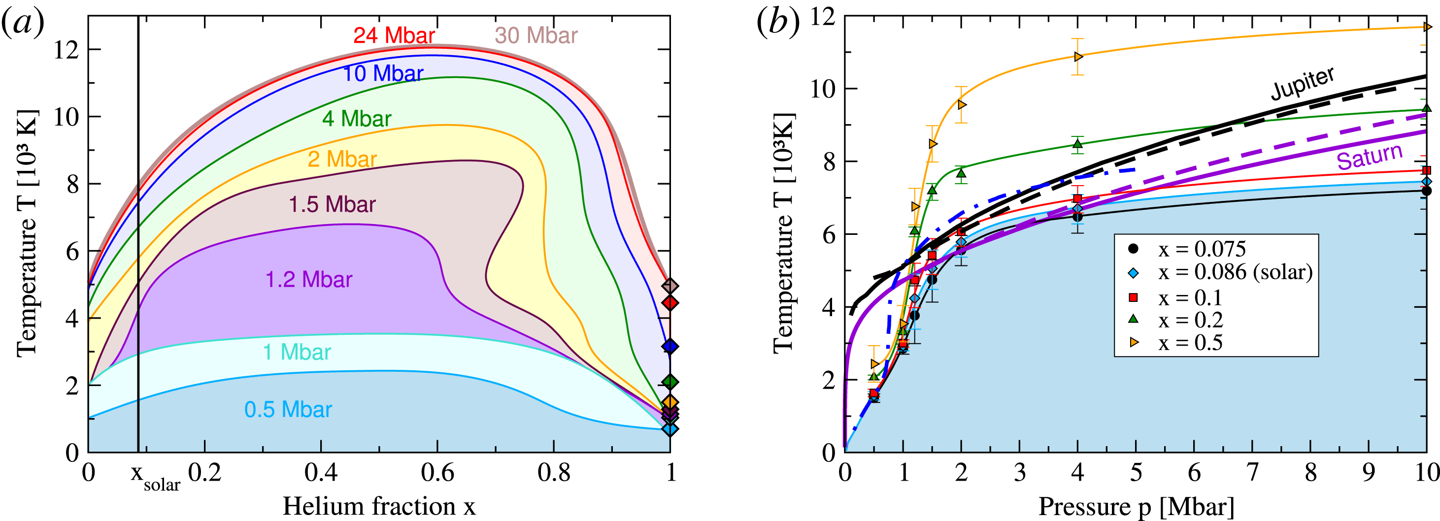
Miscibility diagram for the vdW-DF. (a) Shows demixing temperature as a function of He fraction for the given pressures. Diamonds at
 $x=1$
mark the melting temperature of He for the given pressure. (b) Shows the miscibility diagram in
 $p$
–
 $T$
space for selected helium fractions. Thin solid lines are guides to the eye. Jupiter adiabats are shown for the vdW-DF (thick dashed black line) and the PBE calculations of Militzer & Hubbard (Reference Militzer and Hubbard2013) (thick solid black line). Saturn adiabats are shown for the vdW-DF (thick dashed violet line) and the calculation of Nettelmann, Püstow & Redmer (Reference Nettelmann, Püstow and Redmer2013) (thick solid violet line). The blue dot-dashed line shows the solar demixing conditions obtained with PBE by Morales et al. (Reference Morales, Hamel, Caspersen and Schwegler2013).

In figure 8(a) we show the complete miscibility diagram of hydrogen–helium mixtures calculated using the vdW-DF. Compared to our previous work (Schöttler & Redmer Reference Schöttler and Redmer2018) we added the miscibility region for 30 Mbar. At these pressures, the demixing temperature depends only weakly on pressure. The shown lines are smoothing splines to the actual data points which are available in the original publication (Schöttler & Redmer Reference Schöttler and Redmer2018). In figure 8(b) we show the demixing temperature as a function of pressure for a set of five different He fractions. The demixing region for solar composition is emphasized as the light blue region. Demixing temperatures are an increasingly sharp function of He fraction as evident from figure 8(a). Jupiter and Saturn isentropes are shown, where the thick dashed lines are vdW-DF isentropes with an entropy of
 $s_{\text{J}}=7.613~k_{\text{B}}/\text{atom}$
for Jupiter (Militzer Reference Militzer2013) and
 $s_{\text{S}}=7.357~k_{\text{B}}/\text{atom}$
for Saturn (Hubbard & Militzer Reference Hubbard and Militzer2016). The thick solid black line is the Jupiter isentrope of Militzer & Hubbard (Reference Militzer and Hubbard2013) and the thick solid violet line is the Saturn isentrope of Nettelmann et al. (Reference Nettelmann, Püstow and Redmer2013). Our vdW-DF isentrope for Jupiter is shifted to higher pressures and thus lower temperatures than the PBE isentrope of Militzer & Hubbard (Reference Militzer and Hubbard2013). This shift to higher pressures is already known from the metallization transition in liquid deuterium (see vdW-DF calculations in Knudson et al.
Reference Knudson, Desjarlais, Becker, Lemke, Cochrane, Savage, Bliss, Mattsson and Redmer2015). According to the comparison with QMC data (Clay III et al.
Reference Clay, Holzmann, Ceperley and Morales2016) the error in pressure for the vdW-DF is of the order of 5 % for a Wigner–Seitz radius of
 $r_{\text{s}}=1.34~\text{a}_{0}$
decreasing to approximately 2 % for
 $r_{\text{s}}=1.1~\text{a}_{0}$
while the PBE pressure error is less than 1 % for all Wigner–Seitz radii tested by Clay III et al. (Reference Clay, Holzmann, Ceperley and Morales2016). Thus, if one considers the QMC calculations as the most accurate ab initio simulations, the vdW-DF isentropes will shift towards lower pressures, bringing the Jupiter isentrope in line with that of Militzer & Hubbard (Reference Militzer and Hubbard2013). However, in the absence of highly accurate QMC data for arbitrary densities, temperatures and helium fractions, a quantitative pressure correction is currently not possible. Our vdW-DF Saturn isentrope is not shifted to higher pressures compared to Nettelmann et al. (Reference Nettelmann, Püstow and Redmer2013) and shows slightly higher temperatures, especially for higher pressures. It is currently unclear why the Saturn vdW-DF isentrope is not shifted to higher pressures compared to the PBE isentrope of Nettelmann et al. (Reference Nettelmann, Püstow and Redmer2013) as is the case for Jupiter. The blue dot-dashed line shows the demixing data for solar He abundance obtained using the PBE functional by Morales et al. (Reference Morales, Hamel, Caspersen and Schwegler2013), which intersect the shown Jupiter isentropes because the demixing temperatures are significantly higher compared to the vdW-DF data.
4 Conclusion
In conclusion, we have presented in this paper the details of the miscibility calculations for hydrogen–helium mixtures (see Schöttler & Redmer Reference Schöttler and Redmer2018). The entropy has been calculated using a combination of coupling-constant integration and thermodynamic integration via the equation of state. We have shown that the 2PT-MF method does not yield reliable entropies for H–He mixtures. We have also applied the method of intercepts to calculate the required partial volumes of hydrogen and helium in a H–He mixture. Further, we demonstrated that a reduced coupling-constant integration is able to decrease the computational costs significantly even if the classical pair potentials do not exactly reproduce the DFT system. The free enthalpy of mixing was given for various conditions and the influence of nuclear quantum corrections was discussed. We extended our miscibility diagram to include the demixing region for 30 Mbar, which is close to the 24 Mbar region. Additionally, we calculated a Saturn isentrope based on our vdW-DF data. These data will be used to construct improved interior and evolution models for the gas giants in our solar system and help to solve the long-standing problem of the origin of Saturn’s excess luminosity (see Püstow et al. Reference Püstow, Nettelmann, Lorenzen and Redmer2016). New experiments at novel high-pressure facilities using DACs or FELs will finally benchmark our theoretical predictions.
Acknowledgements
This work was supported by the Deutsche Forschungsgemeinschaft (DFG) within the SPP 1488, SPP 1992 and the SFB 652. Calculations were performed at the IT and Media Centre of the University of Rostock and the North-German Supercomputing Alliance (HLRN). We thank M. Preising for providing the He melting line for the vdW-DF. We also thank N. Nettelmann, M. Bethkenhagen, C. Kellermann and M. French for helpful discussions.