II. MEASUREMENTAL

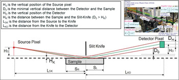
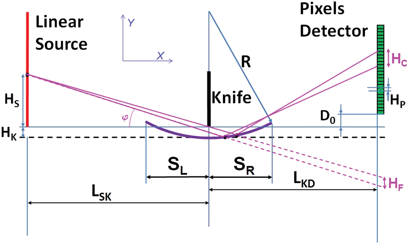
A schematic of the q-XRR setup is shown in Figure 1. The real experimental setup used for the modeling done in this paper is shown in the inset in Figure 1. The linear source has a height of around 10 mm, which at source-to-slit distance (L _SK) of 270 mm provides incident angles in the range 0–37 mrad on the sample. The source emits the CuKα line (8.047 keV). The slit-to-detector distance is 1800 mm. The slit height (H _K) is 30 μm, and the detector is a linear pixel array (1024 pixels, with detector pixel height D _H = 50 μm). This corresponds to a maximum reflection angle of 28 mrad.

Figure 1.

Schematic of the q-XRR setup.

For the purpose of this work, the words “sample” and “mirror” will both be used for describing the reflector. To facilitate comparison of the results from different models, one and the same sample was used for all calculations. A multi-layer sample (10 bi-layers of 3-nm Ni/3-nm C, on a Si substrate) was selected, because it produces X-ray reflectivity scans that have both a Bragg-peak and side-lobes (fringes).

III. MODELING THE EFFECT OF DIFFUSE SCATTERING

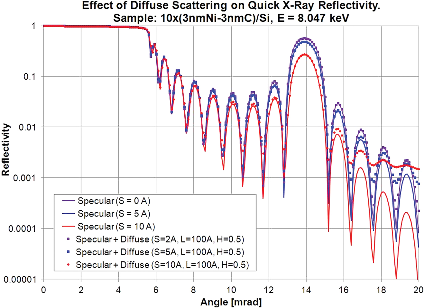
Owing to the use of an extended source and detector in the q-XRR, each detector pixel will see the specular reflection from the corresponding source point plus the diffuse scattering from all source points, i.e. the diffuse scattering contribution has to be integrated over all incident angles φ _In for each specular angle φ _Out. Preliminary results on the contribution of diffuse scattering to the q-XRR scans for a polished surface and a thin film sample were reported by the authors in a previous publication (Stoev et al., Reference Stoev, Samson, Mizusawa and Sakurai2009). Calculations were done using DS2D software (Mizusawa et al., Reference Mizusawa, Stoev and Sakurai2003) and TRDS software (Stepanov, Reference Stepanov2012). The results from modeling the multi-layered sample are shown in Figure 2 for different combinations of vertical roughness S, correlation length L, and Hurst parameter H.

Figure 2.

Effect of diffuse scattering on q-XRR.

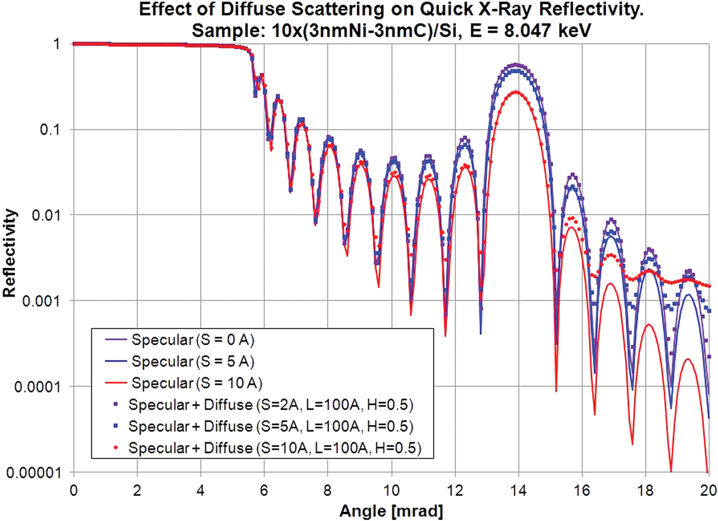
As can be seen, the integrated diffuse scattering does not change significantly the shape of the q-XRR curve up to angles of 15 mrad. Above that angle, the amplitude of the side-lobes is reduced, but their position and width are not changed. Unlike classical scanning X-ray reflectivity, the dynamic range of the detectors for q-XRR is not so wide (usually on the order of 4–4.5 decades for 16-bit digitization). If only the region below 15 mrad is used for fitting and extracting of sample parameters from experimental q-XRR scans, there is no need to include the contribution of diffuse scattering in the modeling function. These results are similar to the ones previously published (Stoev et al., Reference Stoev, Samson, Mizusawa and Sakurai2009).

IV. MODELING THE EFFECTS OF X-RAY BEAM DIVERGENCE

The sample curvature will generally have the same effect on the reflectivity curve as introducing beam divergence. The effects of X-ray beam divergence for the classical X-ray reflectivity setup (with slits/collimators at both source and detector) were modeled with RefleX6 software (Stoev et al., Reference Stoev, Knoth and Schwenke1997; Stoev and Sakurai, Reference Stoev and Sakurai2011).

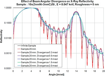
The results are presented in Figure 3, and can be used for comparison with the results of modeling the q-XRR setup with curved samples. As can be seen, the increase in X-ray beam divergence leads to:

• • Reduction in the intensity and increase of the width of the Bragg peak, with practically no change in the position of the Bragg peak.

• • Significant change in the slope of the X-ray reflectivity curve around the critical angle of total reflection.

• • Significant change in the intensity and shift in the position of the high-frequency fringes (also known as side-lobes). These changes are observed both around the Bragg peak and in the region around the critical angle of total reflection.

Figure 3.

Effect of beam divergence in classical X-ray reflectivity.

V. MODELING SAMPLE CURVATURE EFFECTS FOR CONVEX SAMPLES

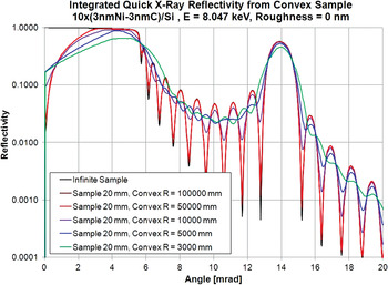
For comparison only, the previously developed software RefleX6 (Stoev et al., Reference Stoev, Knoth and Schwenke1997; Stoev and Sakurai, Reference Stoev and Sakurai2011) was used to model the effects of the radius of curvature for convex samples on the shape of the q-XRR reflectivity curves. As discussed in Stoev and Sakurai (Reference Stoev and Sakurai2011), there are two preferred ways to perform such modeling. The first approach is to use a 2D numerical integration of X-ray reflectivity over the whole sample for each detector point. The sample is divided into N _S sub-intervals and, for each detector pixel and each sample sub-interval, the corresponding source point and reflection angle are calculated. Corrections are made for the shadowing effects because of the knife-slit, self-shadowing because of the mirror curvature, and for the finite sample size. This model correctly accounts for the changing reflection angle from sub-interval to sub-interval and for the detector acceptance angle for each sub-interval. Results from this model are shown in Figure 4.

Figure 4.

Effect of sample curvature on q-XRR scans (numerical integration).

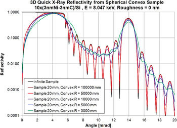
Although very simple and easy to use, the model described above has some disadvantages, and more specifically it assumes a cylindrical sample, not a spherical sample. In order to overcome this deficiency, another model was proposed (Stoev and Sakurai, Reference Stoev and Sakurai2011), which accounts for the 3D shape of the spherical mirror. This is done by using the source image rather than the source itself. For spherical samples at glancing incidence, because the source is very close to the sample, there are very strong aberration effects in forming the source image. Discussion on this subject can be found in Bridou (Reference Bridou1994). Two images will be formed: a tangential image (formed by the rays parallel to the incidence plane); and a sagittal image (formed by the rays perpendicular to the incidence plane). This will lead to blurring of the image, i.e. the image of a line-source will not be a line, but will have a complex 3D shape. At glancing incidence, the position of the sagittal image does not change significantly with the incident angle. On the other hand, the position of the tangential image depends very strongly on the incident angle. The calculation of the reflectivity from a 3D spherical mirror is again based on numerical integration. The source is divided into small sub-sections, the sample is also divided in N _S sub-intervals, and for each source sub-section and sample sub-section, the reflection angle, the tangential image, and the corresponding detector pixel are determined, and the calculated intensity is added to the total intensity for the corresponding detector pixel. For each source sub-section and sample sub-section, the position of the tangential image is used to calculate the correction factor (i.e., correction for different angular density of beam energy because of different divergence for the beams reflected from a flat and convex sub-interval). Results from calculations based on the 3D model are shown in Figure 5. There is no significant difference between the two models for convex samples (see Figures 4 and 5), mainly because convex mirrors always produce beams that have larger divergence than the beams produced by flat mirrors, i.e. there will be a slight reduction of the angular density of beam energy for convex mirrors when compared with flat mirrors.

Figure 5.

Effect of sample curvature on q-XRR scans (3D model).

VI. MODELING SAMPLE CURVATURE EFFECTS FOR CONCAVE SAMPLES

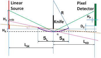
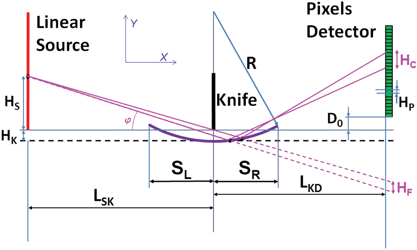
The modeling setup for the q-XRR scans from a concave mirror is shown in Figure 6. In this case, several additional shadowing effects have to be considered:

• • For concave mirrors, it is possible to have sections of the line-source or of the detector that are completely shadowed, i.e. from which no point of the mirror surface is visible. The highest point for these sections is defined as the intersection point of the source (or the detector) with the line through knife-end and mirror-end. For example, in Figure 6, all the points in the brown sections of the source will not “see” any point of the top-surface of the mirror.

• • Self-shadowing of the mirror will occur when some parts of the mirror are blocking other parts of the mirror from seeing the rays from the source (or to the detector). For example in Figure 6, all source points below h(Q) are blocked by the left end of the mirror from seeing the parts of the mirror to the left of point Q.

Figure 6.

q-XRR setup for a concave mirror.

Again, two approaches were considered: 2D numerical integration over a cylindrical concave mirror and 3D numerical integration while accounting for changes in the position of the tangential image. Both methods were implemented in a revised version of the RefleX6 software.

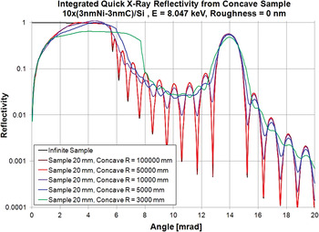
The 2D numerical integration is based on dividing the sample into N _S sub-intervals and, for each detector pixel and each sample sub-interval, calculating the corresponding source point and reflection angle. Corrections are made for all shadowing effects and for the finite sample size. Results from this model are shown in Figure 7. This model correctly accounts for the changing reflection angle from sub-interval to sub-interval, and for the acceptance angle for each sub-interval. The main problem with this model is that it assumes that each mirror sub-section is a flat mirror, i.e. it does not account for the additional beam divergence (or convergence) introduced by the curvature of the mirror sub-section.

Figure 7.

Integrated 2D q-XRR reflectivity for a concave mirror.

For a concave mirror, we can have discontinuities in the tangential image. This was partially discussed in Bridou (Reference Bridou1994). The sagittal and the tangential image points are introduced for convenience only, and do not represent the true “blurred” image as formed by complete ray-tracing of the optical system. The position of the sagittal and tangential image points can be calculated using standard formulas (also known as the Coddington equations):

$$\eqalign{{1 \over d_0} + {1 \over d_{\rm S}} &= {2.\sin \!\lpar \theta \rpar \over R}\comma \; \cr {1 \over d_0} + {1 \over d_{\rm T}} &= {2 \over R\sin \!\lpar \theta \rpar }.}$$

The sign convention is as follows: d ₀, d _S, d _T, and R are positive to the left of the vertex point, and negative to the right of the vertex point, while θ is always positive. For small angles θ, the sagittal image position d _S does not depend significantly on θ, and its value is close to d ₀, while tangential image position d _T depends strongly on θ. There will be an angle θ, for which d _T = ∞, i.e. we will have a discontinuity in the tangential image. This corresponds to having parallel beams, for which no image is formed. Again, these formulas are only an approximation, because they do not consider that many parts of the mirror are involved in the creation of the image.

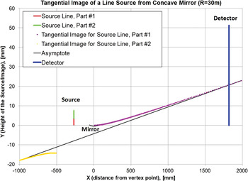
An illustration of this problem is shown in Figure 8, for the case of a concave mirror with a curvature radius of 30 m. This mirror transforms the red part of the source into the purple part of the tangential image (image is “above” the mirror), while the green part of the source is transformed by the mirror into the yellow part of the tangential image (i.e., image is “below” the mirror). The source point between the red and the green part of the source does not produce an image, it produces a parallel beam. The tangential image for the case described above was calculated based on the rays passing through the ends of the mirror.

Figure 8.

Discontinuities in the tangential image.

Another problem is that different parts of the mirror form beams with different divergence, i.e. different tangential images. Also, there are several effects that contribute to the energy density of the beam on the detector pixels for the case of flat and convex mirrors:

• • Different parts of the mirror will contribute to each detector pixel.

• • Different mirror lengths will correspond to the pass-through beam for each source point.

• • A different number of detector pixels will be illuminated by the pass-through beam for each source point.

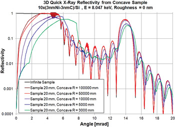
All these effects have to be considered simultaneously when modeling q-XRR scans of concave mirrors. This is done by evaluating the “illuminated” parts of the detector for each source point and each mirror subsection, for both flat (H _F) and concave (H _C) mirrors, as illustrated in Figure 9. The correction factor (H _F/H _C) is used to normalize final results. In addition to this correction, the results have to be normalized in such a way as to ensure that integration of a flat mirror, by following the procedure for integration and correction of a concave mirror will produce the same results as the theoretical reflectivity of a limited flat sample.

Figure 9.

“Illuminated” parts of the detector for flat and concave mirrors.

It should be noted that, for specific cases, H _C could become very close to zero (i.e., the mirror sub-section generates a tangential image onto the detector line, as shown in Figure 8). In these cases, the correction factor becomes very large. To avoid such cases, the maximum value of the correction factor was restricted based on the sizes of the source pixels and detector pixels, and the “nominal” beam spread from a flat sub-section. Even with this restriction, for some values of radius of curvature R and nominal reflection angle θ, there will be large uncertainties in the corrected results, as shown in Figure 10.

Figure 10.

Calculated 3D q-XRR reflectivity for a concave mirror.

Results from the calculation of the q-XRR scans from concave mirrors with different radii of curvature as per the above described procedure are shown in Figure 10. The 3D q-XRR scans are similar to the 2D integrated q-XRR scans presented in Figure 7, but the difference is bigger for the case of concave mirrors than that for convex mirrors (see Figures 4 and 5). This can be attributed to the larger beam divergence from each section for the concave mirrors in comparison to the convex mirrors, i.e. larger changes and discontinuities in the position of the tangential image for the case of a concave mirror.

Generally speaking, the effects of the sample curvature on the shape of the q-XRR scans for concave mirrors are similar to those for convex mirrors. Usually, these effects are significant when the radius curvature, R, is <10 m, and are very similar to the effects of X-ray beam angular divergence in classical X-ray reflectivity (see Figure 3):

• • Reduction in the intensity and increase in the width of the Bragg peak, accompanied with small change in the position of the Bragg peak.

• • Significant change in the shape and the slope of the q-XRR curve around the critical angle of total reflection.

• • Significant change in the intensity and shift in the position of the high-frequency fringes (or side-lobes). These changes are observed both around the Bragg peak and around the critical angle of total reflection.