2. Grad–Shafranov equation

The flux surfaces for an axisymmetric equilibrium must satisfy a Grad–Shafranov equation (Grad & Rubin Reference Grad and Rubin1958; Shafranov Reference Shafranov1957, Reference Shafranov and Leontovich1966) that we find from Ampere’s law and pressure balance by taking the magnetic field to be given by

where ${\it\zeta}$ is the toroidal angle, ${\it\psi}$ is the poloidal flux function, $I=RB_{T}$ with $B_{T}$ the toroidal magnetic field and $R$ the cylindrical radius from the axis of symmetry. The magnetic field is assumed frozen into the flow so that  $c\boldsymbol{{\rm\nabla}}{\it\Phi}=\boldsymbol{V}\times \boldsymbol{B}$ , giving  $\boldsymbol{B}\boldsymbol{\cdot }\boldsymbol{{\rm\nabla}}{\it\Phi}=0$ and requiring the electrostatic potential ${\it\Phi}$ to be a flux function to lowest order.

The kinetic constraints associated with the Fokker–Planck equation (Hinton & Wong Reference Hinton and Wong1985; Catto et al. Reference Catto, Bernstein and Tessarotto1987; Helander Reference Helander2014) require that the temperature be a flux function satisfying

and that the velocity $\boldsymbol{V}$ satisfy

and

As a result, to lowest order $\boldsymbol{V}$ must be toroidal

with ${\it\Omega}=c\,\text{d}{\it\Phi}/\text{d}{\it\psi}$ the toroidal rotation frequency. Notice that (2.4) and (2.5) imply that the toroidal flow (2.7) will not generate pressure anisotropy or give rise to any radial diamagnetic heat flux or radial momentum flux due to gyroviscosity in the short mean-free-path limit (Braginskii Reference Braginskii1958, Reference Braginskii and Leontovich1965).

In addition, we write the gravitational potential $G$ as

with $G_{o}$ the gravitational constant, $r$ the spherical radius and $M_{o}$ the mass of the astrophysical body that is assumed to be a compact source centred at $r=0$ , such that $R=r\sin {\it\vartheta}$ with ${\it\vartheta}$ the angle from the axis of symmetry. Our spherical and cylindrical coordinates are defined to satisfy $r\boldsymbol{{\rm\nabla}}{\it\vartheta}=R\boldsymbol{{\rm\nabla}}{\it\zeta}\times \boldsymbol{{\rm\nabla}}r$ and $\boldsymbol{{\rm\nabla}}z=R\boldsymbol{{\rm\nabla}}R\times \boldsymbol{{\rm\nabla}}{\it\zeta}$ .

Conservation of momentum requires

where $n$ is the ion density and $M$ is the ion mass. The parallel component of this force balance equation is the final kinetic constraint that must be satisfied and is the only place that gravity enters to modify the kinetic constraints of Hinton & Wong (Reference Hinton and Wong1985), Catto et al. (Reference Catto, Bernstein and Tessarotto1987), Helander (Reference Helander2014). Parallel momentum balance requires that the ion density $n$ depends on the poloidal angle

where the density and normalizing or ‘pseudo’ density ${\it\eta}$ are related via the generalized Maxwell–Boltzmann relation that is conveniently written using the exponential factor ${\it\kappa}$ that retains the poloidal dependence due to the centrifugal and gravitational potential,

with $T=T({\it\psi})$ and $p=n(T_{i}+ZT_{e})=2nT$ in a quasi-neutral plasma ( $Zn=n_{e}=\text{electron density}$ ) of ion charge number $Z$ and ion and electron temperatures $T_{i}$ and  $T_{e}$ .

Toroidal momentum balance requires the current density across a flux surface vanish, $\boldsymbol{J}\boldsymbol{\cdot }\boldsymbol{{\rm\nabla}}{\it\psi}=0$ , and then the radial Ampere’s law, $c\boldsymbol{{\rm\nabla}}\times \boldsymbol{B}=4{\rm\pi}\boldsymbol{J}$ requires $I=I({\it\psi})$ . The poloidal Ampere’s law also gives $4{\rm\pi}c^{-1}\boldsymbol{J}\boldsymbol{\cdot }\boldsymbol{{\rm\nabla}}{\it\vartheta}=\boldsymbol{B}\boldsymbol{\cdot }\boldsymbol{{\rm\nabla}}{\it\vartheta}\,\text{d}I/\text{d}{\it\psi}$ . Then the current density can be conveniently decomposed into toroidal and parallel components by writing it as $\boldsymbol{J}=RJ_{\ast }\boldsymbol{{\rm\nabla}}{\it\zeta}+(c/4{\rm\pi})\,\text{d}I/\text{d}{\it\psi}\boldsymbol{B}$ , allowing us to obtain the useful relation $\boldsymbol{J}\boldsymbol{\cdot }\boldsymbol{B}=I\,\boldsymbol{J}\boldsymbol{\cdot }\boldsymbol{{\rm\nabla}}{\it\zeta}+(cB_{P}^{2}/4{\rm\pi}R^{2})\,\text{d}I/\text{d}{\it\psi}$ , with $\boldsymbol{B}_{P}=\boldsymbol{{\rm\nabla}}{\it\psi}\times \boldsymbol{{\rm\nabla}}{\it\zeta}$ the poloidal magnetic field and $B_{P}^{2}=R^{-2}|\boldsymbol{{\rm\nabla}}{\it\psi}|^{2}$ . Combining this result with the $\boldsymbol{{\rm\nabla}}{\it\psi}$ component of force balance, $R^{2}B^{2}\boldsymbol{J}\boldsymbol{\cdot }\boldsymbol{{\rm\nabla}}{\it\zeta}=I\,\boldsymbol{J}\boldsymbol{\cdot }\boldsymbol{B}+c\boldsymbol{{\rm\nabla}}{\it\psi}\boldsymbol{\cdot }[\boldsymbol{{\rm\nabla}}p+Mn(\boldsymbol{{\rm\nabla}}G-{\it\Omega}^{2}R\boldsymbol{{\rm\nabla}}R)]$ , and the toroidal component of Ampere’s law yields the Grad–Shafranov equation (Lovelace et al. Reference Lovelace, Mehanian, Mobarry and Sulkanen1986; Krasheninnikov et al. Reference Krasheninnikov, Catto and Hazeltine2000)

The preceding nonlinear partial differential equation must be solved to find the self-consistent magnetic flux surfaces for an axisymmetric gravitational equilibrium in the presence of hot, toroidal rotating plasma. The expression is simpler than that given in Lovelace et al. (Reference Lovelace, Mehanian, Mobarry and Sulkanen1986) because poloidal flows are not allowed to lowest order by the kinetic constraints on a drifting Maxwellian solution of the Fokker–Planck equation. However, poloidal flows are allowed by the ideal MHD equations (Lovelace et al. Reference Lovelace, Mehanian, Mobarry and Sulkanen1986; Prasanna et al. Reference Prasanna, Tripathy and Das1989; Ogilvie Reference Ogilvie1997; McClements & Thyagaraya Reference McClements and Thyagaraya2001; Throumoulopoulos & Tasso Reference Throumoulopoulos and Tasso2001) since they ignore diamagnetic heat flow and gyroviscosity.

3. Separable form

To find a separable form for the Grad–Shafranov equation we assume

where ${\it\mu}=\cos {\it\vartheta}$ and our normalization is $H({\it\mu}=0)=1$ . We will see that the parameter ${\it\alpha}$ plays the role of an eigenvalue that is determined by solving the Grad–Shafranov equation. The vacuum limit $H=1-{\it\mu}^{2}$ recovers a homogeneous magnetic field for ${\it\alpha}=-2$ and a point dipole solution if ${\it\alpha}=1$ , where ${\it\psi}_{o}$ is a constant reference value at the reference location $R_{o}$ (reference values are defined at the equatorial plane ${\it\mu}=0$ and denoted by a subscript ‘ $o$ ’).

We obtain an ordinary differential equation for $H$ by assuming

with $n_{o}=n({\it\psi}={\it\psi}_{o},{\it\mu}=0)$ and ${\it\kappa}_{o}={\it\kappa}({\it\mu}=0)$ . Notice that the rotation frequency and temperature increase as $r\rightarrow 0$ , and for ${\it\alpha}<-3/2$ the density increases as $r\rightarrow \infty$ , while for ${\it\alpha}<-2$ the toroidal magnetic field increases as $r\rightarrow \infty$ . In addition, the poloidal magnetic field

vanishes as $r\rightarrow 0$ for ${\it\alpha}<-2$ .

Defining the positive constants

and

an ordinary second-order nonlinear differential equation for $H$ is obtained from (2.12) (Krasheninnikov et al. Reference Krasheninnikov, Catto and Hazeltine2000):

where

with ${\it\beta}$ defined using the poloidal magnetic field rather than the full magnetic field. Equation (3.11) with (3.12) inserted is an ordinary nonlinear second-order differential equation for the flux function, and therefore much easier to solve than the full Grad–Shafranov equation (2.12). In this self-similar limit, strict Keplerian motion corresponds to ${\it\omega}^{2}=g/2$ . The normalizations here differ from Catto & Krasheninnikov (Reference Catto and Krasheninnikov2015) since $g$ replaces $g/{\it\beta}$ and ${\it\omega}^{2}$ replaces ${\it\omega}^{2}/{\it\beta}$ .

Some solutions to this Grad–Shafanov equation can be found by the techniques illustrated in Krasheninnikov et al. (Reference Krasheninnikov, Catto and Hazeltine1999, Reference Krasheninnikov, Catto and Hazeltine2000), Catto & Krasheninnikov (Reference Catto and Krasheninnikov2015) and references therein, however, some care is needed. Moreover, new solutions not considered previously will be the main focus of the next section. We desire the solution $H$ to be up–down symmetric having the normalization $H({\it\mu}=0)=1$ , satisfying the boundary condition $H({\it\mu}^{2}=1)=0$ and having no zero crossings for $1>{\it\mu}^{2}\geqslant 0$ . Solutions with zero crossings exist, but poloidal magnetic field reversal is considered in a separate investigation (Krasheninnikov & Catto Reference Krasheninnikov and Catto2015). Moreover, up–down asymmetric solutions are possible, but will not be considered herein.

When $G=0$ , an exact solution to (3.11) and (3.12) exists even in the presence of a toroidal magnetic field and is given by (Catto & Krasheninnikov Reference Catto and Krasheninnikov2015)

with

To obtain this solution it is helpful to notice that

Importantly, gravity forces us to assume ${\it\alpha}<0$ to avoid singular behaviour as $H({\it\mu}^{2}\rightarrow 1)\rightarrow 0$ . Consequently, we will only consider ${\it\alpha}<0$ , and remark that the effects of gravity only enter through the exponential factor $\text{e}^{-g}$ as ${\it\mu}^{2}\rightarrow 1$ . If we assume that

with $C$ a positive constant to be determined, then as ${\it\mu}^{2}\rightarrow 1$ , we obtain the relation

Consequently, we expect ${\it\alpha}+2<0$ unless $b^{2}>{\it\beta}{\it\omega}^{2}$ . This condition means that a toroidal magnetic field is required to obtain ${\it\alpha}>-2$ to make both components of the magnetic field vanish at infinity, while for ${\it\alpha}+2<0$ these components vanish as $r\rightarrow 0$ .

4. Strong gravity solutions at high ${\it\beta}$

Examining (3.11) indicates that a simple solution might be possible for strict Keplerian motion in the limit of a vanishing magnetic field. In this limit $2{\it\omega}^{2}=g$ , ${\it\beta}\rightarrow \infty$ , and $b^{2}\sim 1$ , and it appears that the left-hand side of (3.11) can be ignored. The resulting cubic equation,

with $2{\it\omega}^{2}=g$ , then has the simple solution,

with ${\it\alpha}=-2$ . However, this solution fails as ${\it\mu}^{2}\rightarrow 1$ since the left side cannot be ignored in (3.11). In fact, the ${\it\mu}^{2}\rightarrow 1$ solution must be of the form (3.16) and (3.17), with the $b^{2}$ terms ignored. Then (3.17) becomes

The preceding indicates that only solutions with ${\it\alpha}+2<0$ are possible in this limit. To see that this is indeed the case, we can solve the cubic (4.1) for ${\it\omega}^{2}\rightarrow \infty$ , $g\rightarrow \infty$ and ${\it\beta}\rightarrow \infty$ . Using $H({\it\mu}=0)=1$ , (4.1) requires

From (4.3) and (4.4) we see that we will only be interested in $2{\it\omega}^{2}>g$ in this section, and since ${\it\alpha}+2<0$ the flux surfaces will bow out at the equatorial plane. The cubic has three real and unequal roots. In particular, the root of interest, as ${\it\mu}^{2}\rightarrow 1$ , goes like

which smoothly matches onto (3.16) when the left-hand side of the Grad–Shafranov equation (3.11) is retained provided (4.3) is satisfied. We can then see the left-hand side of (3.11) is unimportant only if

In this case (4.3) and (4.4) are consistent only when

Using (4.7) in (4.6) gives the inequality

Figure 1.

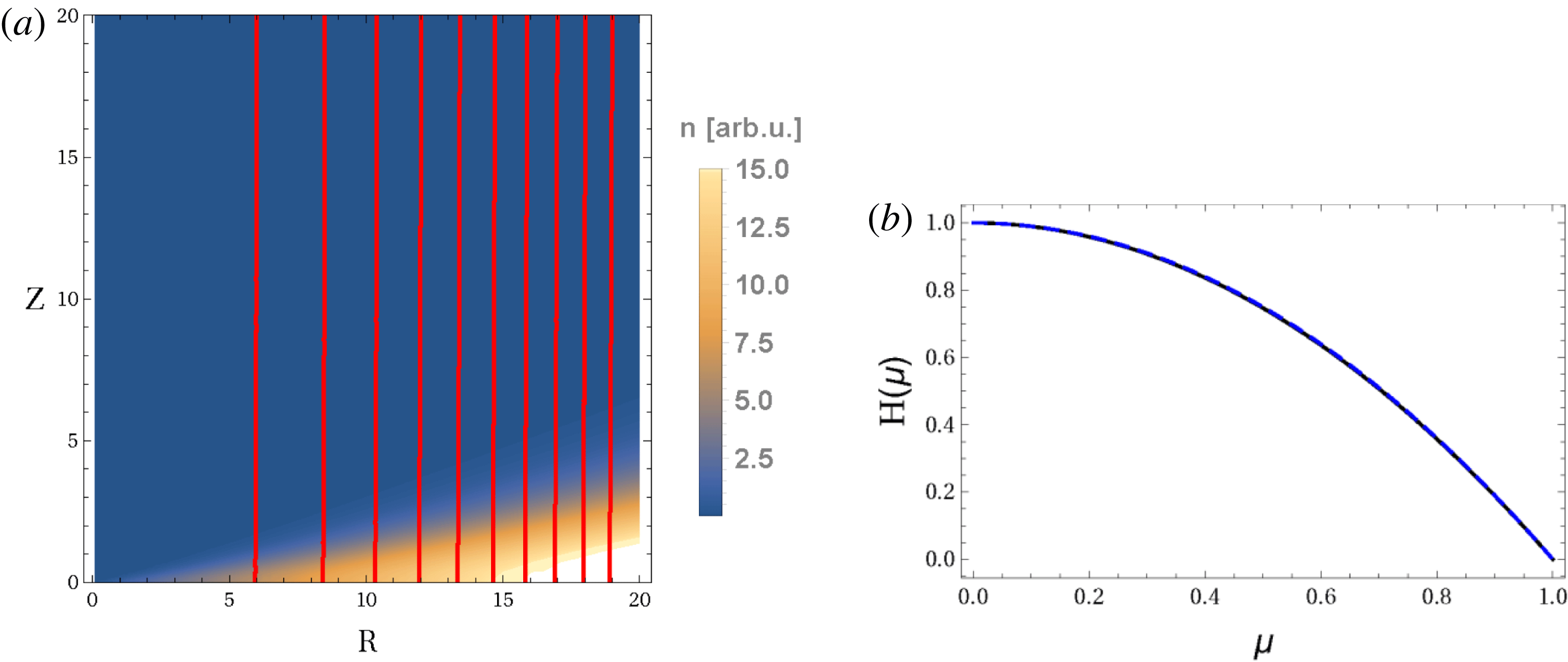
Parameters $g=2$ , ${\it\omega}^{2}=2$ , ${\it\beta}=300$ and $b^{2}=0$ , giving ${\it\alpha}=-3.002$ . (a) Magnetic surfaces (red curves) and density (colour shading) as functions of $R$ and $Z$ . The density is normalized to unity at $R=1$ and $Z=0$ . (b) The solution $H({\it\mu})$ is plotted versus ${\it\mu}$ . The numerical result is shown with the solid curve, the solution of the cubic equation (4.1) is dashed (and barely discernible), and the approximate expression (4.2) with ${\it\alpha}=-3.002$ is shown for reference with dotted line.

A thin equatorial plane plasma disk requires $g\gg 1$ and is not allowed when (4.8) holds. This thin disk inequality (4.8) is found by inserting the cubic (4.1) and (4.4) into the Maxwell–Boltzmann density factor (3.12), using $H$ from (4.2), and then expanding about the equatorial plane

The preceding gives a plasma disk width or height ${\it\Delta}$ of

since in the vicinity of the equatorial plane ${\it\mu}^{2}\approx z^{2}/R^{2}$ .

When (4.8) is satisfied, the solution of the cubic equation (4.1) gives a global solution to the Grad–Shafranov equation (3.11) for all ${\it\vartheta}$ angles. For example, if we take ${\it\beta}=300$ , $g=2={\it\omega}^{2}$ , then inequality (4.8) is satisfied. Then the cubic is quite a good solution with ${\it\alpha}=-3$ and $C=2$ from (4.4) and (4.7), but with no significant plasma disk since $2/g=1$ . The numerical solution of (3.11) gives several solutions near ${\it\alpha}=-3$ , with the one having the least deviation from the cubic solution having ${\it\alpha}=-3.002$ . Figure 1(a) shows flux surfaces and density contours for this solution, while figure 1(b) plots $H$ versus ${\it\mu}$ for the same. The full numerical solution is also compared to the cubic solution, and the crude solution from (4.2) for ${\it\alpha}=-3.002$ . The exact numerical and the full cubic solution are in excellent agreement, while the departure from the crude solution indicates that approximation (4.2) is not valid since ${\it\alpha}$ is too far from $-2$ . To improve the agreement with (4.2) we need to only pick $2{\it\omega}^{2}$ closer to  $g$ . The other solutions near ${\it\alpha}=-3$ have similar behaviour, but the agreement with the cubic limit is not quite as good. We also find that as we let $2{\it\omega}^{2}$ become closer to  $g$ , the numerical solution is quite oscillatory about the simple solution (4.2).

As $2{\it\omega}^{2}\rightarrow g$ , inequality (4.8) cannot be satisfied for fixed ${\it\beta}$ and  $g$ . For example, returning to ${\it\beta}=300$ and $g=2$ , but letting ${\it\omega}^{2}=1.017$ we find the inequality is not even close to being satisfied so we expect the cubic solution will be inadequate. In such cases the full expression (4.3) remains valid, but it is no longer possible to assume the cubic holds all the way from the equatorial plane to the poles. However, the cubic can remain valid in the plasma disk when $2{\it\omega}^{2}>g$ and ${\it\beta}\gg 1\sim b^{2}$ . But once outside the disk the solution for $H$ will be more complicated. Taking ${\it\beta}=10$ , $g=20$ and ${\it\omega}^{2}=12$ , for example, gives ${\it\alpha}=-4$ and a disk width of ${\it\Delta}=0.32R$ but completely violates inequality (4.8). 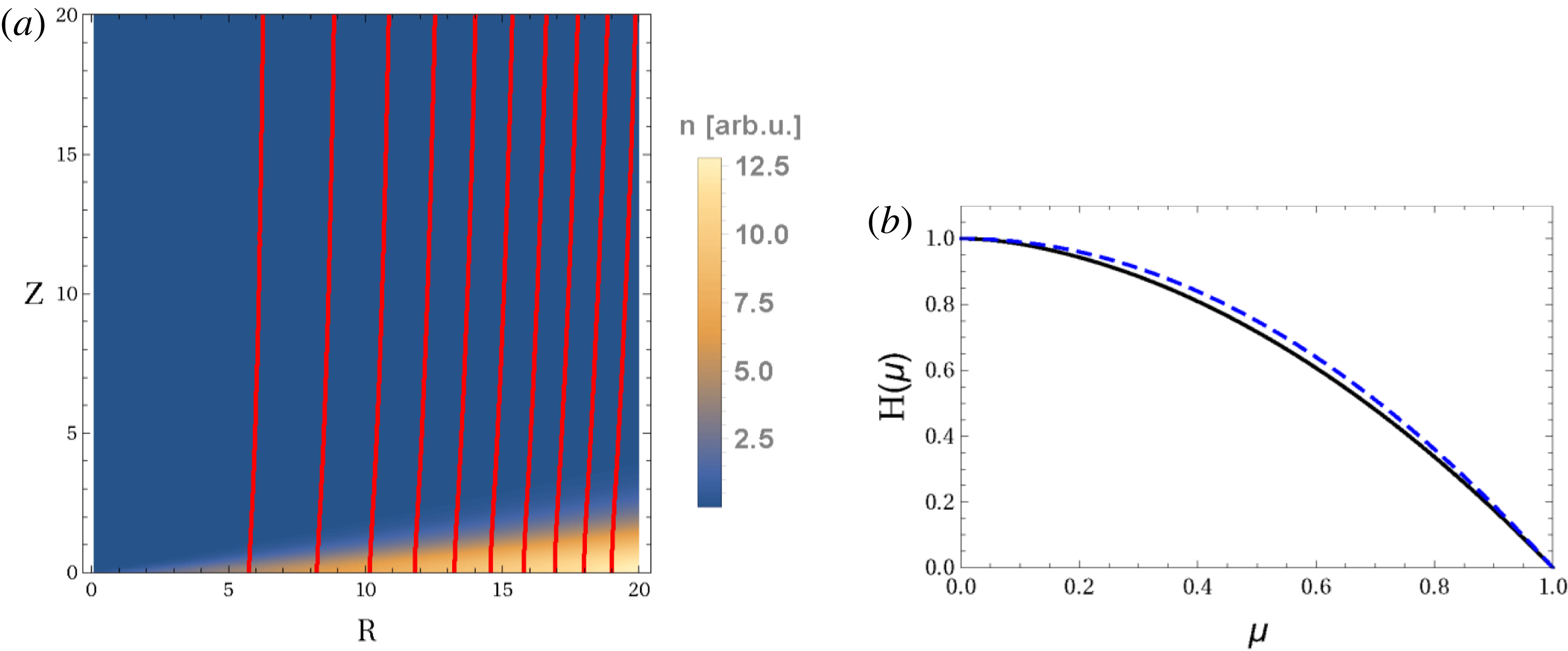As a result, the cubic solution is unable to reproduce the oscillatory structure outside the disk (where $\text{d}^{2}H/\text{d}{\it\mu}^{2}$ is small) seen in the full numerical solution of figure 2(a,b), for which ${\it\alpha}=-4.32$ and there is clearly some disk localization about the equatorial plane with a width of ${\it\Delta}\approx 0.55R$ .

Figure 2.

Parameters $g=20$ , ${\it\omega}^{2}=12$ , ${\it\beta}=10$ and $b^{2}=0$ , giving ${\it\alpha}=-4.32$ . (a) Magnetic surfaces (red curves) and density (colour shading) as functions of $R$ and $Z$ . The density is normalized to unity at $R=1$ and $Z=0$ . (b) The solution $H({\it\mu})$ is plotted versus ${\it\mu}$ . The numerical result is shown with the solid curve, the solution of the cubic equation (4.1) is dashed, and the approximate expression (4.2) with ${\it\alpha}=-4.32$ is shown for reference with dotted line.

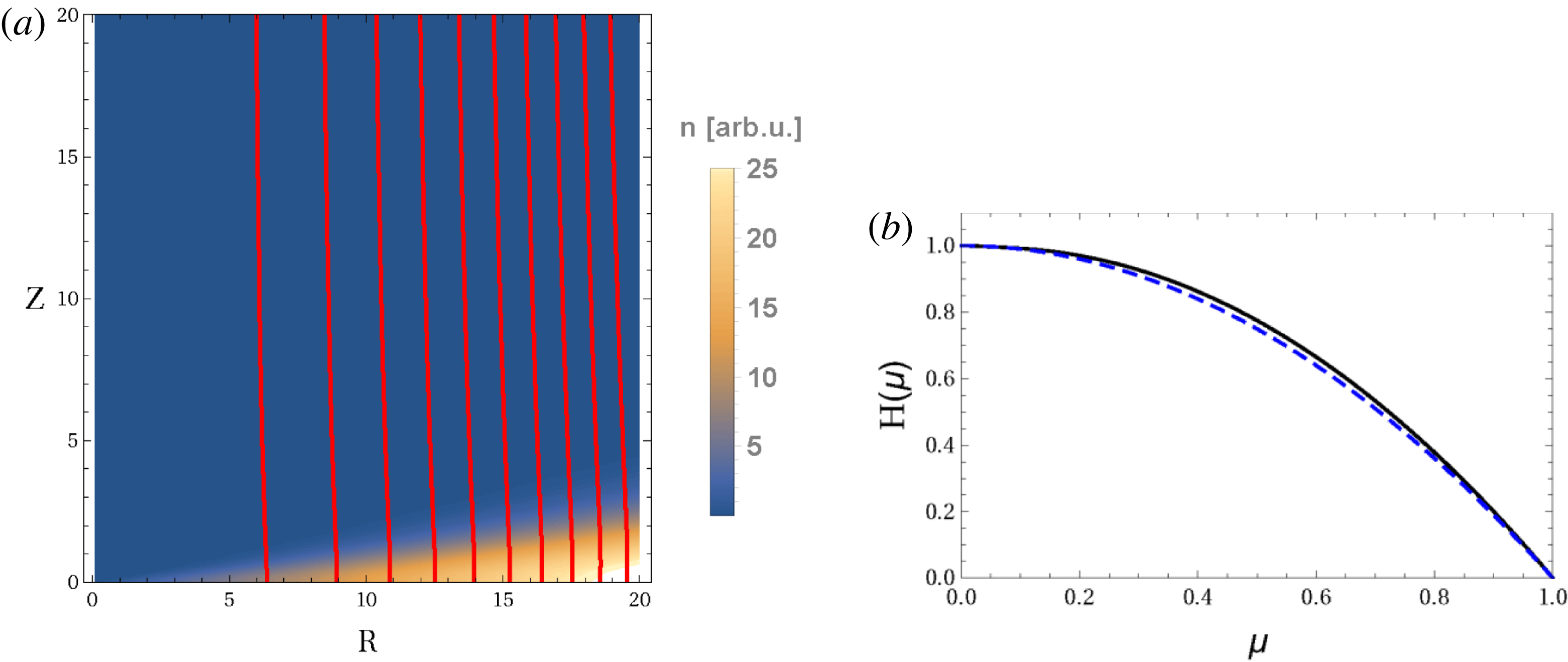
To satisfy (4.8) and obtain some minor localization about the equatorial plane we need $2/g<1$ . For example, taking ${\it\beta}=1600$ and $g=4={\it\omega}^{2}$ , gives $2/g=1/2$ , where the left and right-hand sides of (4.8) are comparable, so we are not satisfying the inequality. In this case (4.4) and (4.7) give ${\it\alpha}=-4$ , ${\it\Delta}=0.71R$ and $C=2$ . The full numerical solution is shown in figure 3(a,b) for these parameters and gives ${\it\alpha}=-4.002$ with ${\it\Delta}\approx 0.7R$ . The cubic solution and the crude approximation of (4.2) with ${\it\alpha}=-4.002$ are also plotted for $H$ in figure 3(b). The agreement is again extremely good, except for the crude analytic result that is shown for reference.

Figure 3.

Parameters $g=4$ , ${\it\omega}^{2}=4$ , ${\it\beta}=1600$ and $b^{2}=0$ , giving ${\it\alpha}=-4.002$ . (a) Magnetic surfaces (red curves) and density (colour shading) as functions of $R$ and $Z$ . The density is normalized to unity at $R=1$ and $Z=0$ . (b) The solution $H({\it\mu})$ is plotted versus ${\it\mu}$ . The numerical result is shown with the solid curve, the solution of the cubic equation (4.1) is dashed (again barely detectable), and the approximate expression (4.2) with ${\it\alpha}=-4.002$ is shown for reference with dotted line.

This last case suggests that the cubic may still be a reasonably good solution even when

Assuming this is the case (4.3) becomes

If we consider $g\gg 1$ , but for simplicity take $C=1$ , then these become

and

To also satisfy (4.4) we need ${\it\omega}^{2}=g$ . Assuming ${\it\omega}^{2}=g$ we try $2/g=1/4$ so ${\it\Delta}=R/2$ , then ${\it\beta}=\text{e}^{8}$ , $g=8={\it\omega}^{2}$ and ${\it\alpha}+2=-{\it\omega}^{2}/2=-4$ . Figure 4(a,b) give the numerical results for this case which gives ${\it\alpha}$ very close to $-6$ ( ${\it\alpha}=-5.9997$ ) and ${\it\Delta}=0.9R$ instead of ${\it\Delta}=0.5R$ . The numerical solution has barely discernible oscillations about the cubic solution in this case. In addition to the cubic solution, we plot (4.2) with ${\it\alpha}=-5.9997$ for reference in (b).

Figure 4.

Parameters $g=8$ , ${\it\omega}^{2}=8$ , ${\it\beta}=300$ , ${\it\beta}=\text{e}^{8}$ and $b^{2}=0$ , giving ${\it\alpha}=-5.9997$ . (a) Magnetic surfaces (red curves) and density (colour shading) as functions of $R$ and $Z$ . The density is normalized to unity at $R=1$ and $Z=0$ . (b) The solution $H({\it\mu})$ is plotted versus ${\it\mu}$ . The numerical result is shown with the solid curve, the solution of the cubic equation (4.1) is dashed (barely discernible), and the approximate expression (4.2) with ${\it\alpha}=-5.9997$ is shown for reference with dotted line.

To seek solutions for $C$ more generally we combine (4.3) and (4.4) to eliminate ${\it\alpha}+2$ and obtain

which can almost be satisfied in the strict Keplerian limit $2{\it\omega}^{2}\rightarrow g$ if the exponential also goes to zero. This suggests looking at large $C$ such that ${\it\omega}^{2}/C\rightarrow g/2C\ll 1$ , where we also want $g\gg 2$ for a disk equilibrium. Assuming $(1-g/2{\it\omega}^{2})^{-1}\gg C\gg g/2\gg 1$ the preceding reduces to

for which the cubic solution is not expected to be valid outside the disk. The preceding inequalities and (4.16) suggest picking numbers to satisfy

provided $(1-g/2{\it\omega}^{2})^{-1}\gg {\it\beta}^{1/3}\gg g/2\gg 1$ . To obtain figure 5(a,b) we take ${\it\beta}=1000$ and $g=6$ . Then, according to (4.17), we must allow $2{\it\omega}^{2}$ to become quite close to $g$ such that ${\it\alpha}\rightarrow -2$ . For example, choosing $(1-g/2{\it\omega}^{2})=10^{-6}$ satisfies the inequalities and gives $C\approx 50$ , as well as ${\it\alpha}\rightarrow -2$ . However, this is a limit in which the cubic solution is only valid in the disk so the behaviour of $H$ must be found numerically outside the disk. The numerical solution found for ${\it\alpha}=-2.174$ displays strong oscillatory behaviour about the cubic solution, as is shown in figure 5(b) along with the reference solution of (4.2) for ${\it\alpha}=-2.174$ .

Figure 5.

Parameters $g=6$ , ${\it\omega}^{2}=3\cdot (1+10^{-6})$ , ${\it\beta}=1000$ and $b^{2}=0$ , at ${\it\alpha}=-2.174$ . (a) Magnetic surfaces (red curves) and density (colour shading) as functions of $R$ and $Z$ . The density is normalized to unity at $R=1$ and $Z=0$ . (b) The solution $H({\it\mu})$ is plotted versus ${\it\mu}$ . The numerical result is shown with the solid curve, the solution of the cubic equation (4.1) is dashed, and the approximate expression (4.2) with ${\it\alpha}=-2.174$ is shown for reference with dotted line.

We remark that the numbers have been chosen to indicate the wide variety of Grad–Shafranov solutions to (3.11) and (3.12) that are possible at large ${\it\beta}$ . Many more solutions are possible than the few that are shown. For example, we have not considered the limit $b^{2}>{\it\beta}{\it\omega}^{2}\sim {\it\beta}g/2\gg {\it\beta}\gg 1$ , which requires a very strong toroidal magnetic field, but allows the magnetic field to vanish at infinity. In the next section we will focus on lower ${\it\beta}$ solutions found in Catto & Krasheninnikov (Reference Catto and Krasheninnikov2015) and present further numerical solutions.

5. Other gravitational solutions

In this section we will demonstrate analytically and numerically that at lower ${\it\beta}$ , it is possible to find thin plasma disks about the equatorial plane provided a toroidal magnetic field is retained. A toroidal magnetic field was not retained in Catto & Krasheninnikov (Reference Catto and Krasheninnikov2015) but is required in all cases to find a numerical solution with ${\it\alpha}>-2$ . Fortunately, it is easily added to the analytic results presented there.

To begin, we generalize (to a degree) the integral constraint obtained from the Grad–Shafranov equation to include the toroidal magnetic field:

Using the vacuum magnetic field solution for the ${\it\alpha}=-2$ root of $H=1-{\it\mu}^{2}$ , we find that the ${\it\beta}\sim b^{2}\ll 1$ and ${\it\beta}g\sim {\it\beta}{\it\omega}^{2}\ll 1$ corrections to that result must satisfy

For $g\ll 1$ , only a weak density departure from cylindrical symmetry is allowed giving

Recall from (3.17) that $b^{2}>{\it\beta}{\it\omega}^{2}$ is required for a solution that keeps $0>{\it\alpha}>-2$ , thereby making the poloidal magnetic field fall off at large distances and pinch in slightly at the equatorial plane. Even in this small $g$ limit finite $b^{2}>{\it\beta}{\it\omega}^{2}$ is required to find a numerical solution for ${\it\alpha}>-2$ .

A more interesting ${\it\beta}g\sim {\it\beta}{\it\omega}^{2}\ll 1$ limit is $g\sim {\it\omega}^{2}\gg 1$ and ${\it\beta}\sim b^{2}\ll 1$ which introduces strong poloidal density variation and for which the integral constraint yields

These results are the same as in Catto & Krasheninnikov (Reference Catto and Krasheninnikov2015), except the toroidal field term has been retained and it further enhances the pinching in of the flux surfaces at the equatorial plane. The disk thickness from $\text{e}^{-g{\it\mu}^{2}/2}$ is as given by (4.10). Result (5.4) is verified by a numerical solution as shown in figure 6(a,b) for ${\it\beta}=0.001$ , $g=100$ , ${\it\omega}^{2}=4$ and $b^{2}=0.05$ . Analytically we find ${\it\alpha}=-1.992$ and ${\it\Delta}/R=0.14$ and numerically we obtain ${\it\alpha}=-1.993$ and ${\it\Delta}/R=0.12$ . We need $b^{2}>{\it\beta}{\it\omega}^{2}$ in this limit to satisfy (3.17). Otherwise no solution is possible for ${\it\alpha}+2>0$ as confirmed numerically. Equation (5.4) remains valid in the strict Keplerian case $g=2{\it\omega}^{2}\gg 1$ , where we can evaluate the integrals in (5.2) a little more carefully to find ${\it\alpha}+2\simeq (b^{2}-{\it\beta}/4)({\rm\pi}/2g)^{1/2}$ . When $1\gg b^{2}\gg {\it\beta}$ , this reduces to (5.4). The numerical solution confirms that the strict Keplerian case is a valid limit.

Figure 6.

Parameters $g=100$ , ${\it\omega}^{2}=40$ , ${\it\beta}=0.001$ and $b^{2}=0.05$ , giving ${\it\alpha}=-1.993$ . (a) Magnetic surfaces (red curves) and density (colour shading) as functions of $R$  and  $Z$ . The density is normalized to unity at $R=1$ and $Z=0$ . (b) The solution $H({\it\mu})$ is plotted versus ${\it\mu}$ . The numerical (solid) curve and the reference $1-{\it\mu}^{2}$ (dashed) curve are indistinguishable.

Catto & Krasheninnikov (Reference Catto and Krasheninnikov2015) find more general disk solutions localized to the equatorial plane by considering $g>2{\it\omega}^{2}$ and then allowing $g-2{\it\omega}^{2}\gg 1$ with $g\gg b^{2}\sim 1\gg {\it\beta}$ , so that the exponential dependence $\text{e}^{{\it\chi}}$ in the Grad–Shafranov equation provides the desired localization about ${\it\mu}=0$ . Therefore we follow their treatment to find disk solutions with strong poloidal variation but with the toroidal magnetic field retained. To do so, we need to find a solution in the disk different from the solution $H=(1-{\it\mu}^{2})^{-{\it\alpha}/2}$ valid outside the disk. We find this inner solution as in Catto & Krasheninnikov (Reference Catto and Krasheninnikov2015) by solving the approximate Grad–Shafranov equation

where now both rotation and gravity enter the exponential density dependence, for which we use

When $g-2{\it\omega}^{2}\gg 1$ we obtain strong exponential decay away from the equatorial plane with the possibility of $0>{\it\alpha}>-2$ provided $b^{2}>{\it\beta}{\it\omega}^{2}$ according to (3.17). As already noted, this constraint from (3.17) was not considered in Catto & Krasheninnikov (Reference Catto and Krasheninnikov2015). Notice that for $0>{\it\alpha}>-2$ , $\text{d}^{2}H/\text{d}{\it\mu}^{2}<0$ in (5.5) if ${\it\beta}(g-2{\it\omega}^{2})+2b^{2}>0$ . More importantly, for $0>{\it\alpha}>-2$ we need $b^{2}>{\it\beta}{\it\omega}^{2}$ to satisfy (3.17). For the solutions given from this point on we expect $\text{d}^{2}H/\text{d}{\it\mu}^{2}<0$ and $H\leqslant 1$ for all $1\geqslant {\it\mu}^{2}\geqslant 0$ . These observations suggest, in agreement with Catto & Krasheninnikov (Reference Catto and Krasheninnikov2015), that these solutions which are strongly localized to the equatorial plane in the presence of gravity are not possible for $g<2{\it\omega}^{2}$ and $0>{\it\alpha}>-2$ since the rotation is too strong for the plasma to be gravitationally confined.

Continuing as in Catto & Krasheninnikov (Reference Catto and Krasheninnikov2015), we multiply (5.5) by $\text{d}H/\text{d}{\it\mu}$ and integrate from $H=1$ (at ${\it\mu}=0$ ) to $H<1$ (for ${\it\mu}^{2}>0$ ) to find

where we select the negative root to make $\text{d}H/\text{d}{\it\mu}<0$ . Using $\int \,\text{d}x/\sqrt{1-\text{e}^{-x}}=2\tanh ^{-1}\sqrt{1-\text{e}^{-x}}$ we obtain

where ${\it\sigma}\equiv \sqrt{{\it\beta}(g-2{\it\omega}^{2})[g-2{\it\omega}^{2}-2({\it\alpha}+2)-2({\it\alpha}+1)b^{2}/{\it\beta}]}$ and the upper (lower) sign is for ${\it\mu}>0$ ( ${\it\mu}<0$ ). A solution strongly localized at the equatorial plane is found for $-x=(g-2{\it\omega}^{2})(1-H)/{\it\alpha}\gg 1$ that results in only a small departure from the gravity-free solution $H=(1-{\it\mu}^{2})^{-{\it\alpha}/2}$ that remains an adequate approximation in the outer region. The behaviour $x\approx \mp {\it\sigma}{\it\mu}\approx \mp {\it\sigma}z/R$ implies a disk width ${\it\Delta}=R/{\it\sigma}$ so that ${\it\sigma}\gg 1$ is required. Moreover, as ${\it\beta}$ increases, $H-1$ extends toward ${\it\mu}^{2}=1$ as seen from $-x=(g-2{\it\omega}^{2})(1-H)/{\it\alpha}\gg 1$ , making $\text{d}^{2}H/\text{d}{\it\mu}^{2}$ small since $H-1\propto \mp {\it\mu}$ .

Using (5.7) and (5.8) on the right-hand side of the integral constraint (5.1) with ${\it\alpha}\approx -2$ , and the vacuum solution $H=1-{\it\mu}^{2}$ inserted on the left-hand side yields

The corresponding disk width is given by

requiring $1/(g-2{\it\omega}^{2})\ll {\it\beta}(g-2{\it\omega}^{2}+2b^{2}/{\it\beta})\ll (g-2{\it\omega}^{2})$ . Strict Keplerian motion is not allowed in this low ${\it\beta}$ thin disk limit. Figure 7(a,b) shows the flux surfaces, density contours and $H$ for ${\it\beta}=0.01$ , $g=200$ , ${\it\omega}^{2}=50$ and $b^{2}=0.5$ , for which the analytic and numerical results give ${\it\Delta}/R=0.071$ . The ${\it\alpha}$ values are close as well, with ${\it\alpha}=-1.86$ analytically and ${\it\alpha}=-1.93$ numerically. In (b) we also plot $H=1-{\it\mu}^{2}$ for reference.

Figure 7.

Parameters $g=200$ , ${\it\omega}^{2}=50$ , ${\it\beta}=0.01$ and $b^{2}=0.5$ , giving ${\it\alpha}=-1.93$ . (a) Magnetic surfaces (red curves) and density (colour shading) as functions of $R$ and  $Z$ . The density is normalized to unity at $R=1$ and $Z=0$ . (b) The solution $H({\it\mu})$ is plotted versus ${\it\mu}$ . The numerical result is shown as the solid curve, and $1-{\it\mu}^{2}$ is shown dashed for reference.

Numerically, it is possible, but difficult, to find solutions that make the density decrease with radius ( ${\it\alpha}>-1.5$ ), so we have not found solutions for ${\it\alpha}\rightarrow 0$ , as claimed in Catto & Krasheninnikov (Reference Catto and Krasheninnikov2015), even for finite $b^{2}$ .

6. Strict Keplerian solution

All of the solutions found so far in § 4 break down for the strict Keplerian motion case of $g=2{\it\omega}^{2}$ . In this section, we will discuss this special and particularly interesting case and demonstrate that thin disk equilibrium solutions are possible. To do so, we consider the limit $2{\it\omega}^{2}=g$ and $b^{2}=0$ for large ${\it\beta}$ . As in § 4, this order means that near the equatorial plane $H=(1-{\it\mu}^{2})^{-{\it\alpha}/3}$ as in (4.2) is the inner solution. However, unlike § 4, the left-hand side of (3.11) is important, so (4.1) is not valid at ${\it\mu}=0$ . Therefore, (4.4) does not hold. Instead, $g$ is so large that the equatorial plane plasma disk is very thin and the large $g$ inner solution transitions to the cylindrical outer solution $H=(1-{\it\mu}^{2})^{-{\it\alpha}/2}$ of (3.13) very near the equatorial plane.

When either (3.13) or (4.2) is inserted into the Maxwell–Boltzmann exponential factor and expanded for small ${\it\mu}$ , the result is ${\it\chi}\simeq -g{\it\mu}^{2}/2$ . Then, because $g=2{\it\omega}^{2}$ and ${\it\beta}$ are so large, the leading correction to these terms from just outside the thin equatorial plane disk must be retained since they only cancel in the inner region. Therefore, using ${\it\alpha}\approx -2$ and $H=1-{\it\mu}^{2}$ , (5.1) becomes

Rearranging, we estimate the eigenvalue for these cases to be

The disk thickness ${\it\Delta}$ for this limit is given by (4.10) due to the Maxwell–Boltzmann behaviour.

Figure 8(a,b) show very strong gravity strict Keplerian, high ${\it\beta}$ numerical results for $g=2{\it\omega}^{2}=200$ , ${\it\beta}=10$ and $b^{2}=0$ . We also show $H=1-{\it\mu}^{2}$ in figure 8(b) for reference. The numerical value found for ${\it\alpha}$ is $-2.06$ while the analytic value from (6.2) is $-2.12$ . Both numerically and analytically we find ${\it\Delta}/R=(2/g)^{1/2}=0.1$ . As $1/g$ becomes larger, the disk becomes more diffuse as expected, and the flux surfaces oscillate about $H=1-{\it\mu}^{2}$ . Based on the estimate (6.2) and numerical solutions, we find that strict Keplerian solutions do not have thin plasma disks for ${\it\alpha}<-2.25$ .

Figure 8.

Parameters $g=200$ , ${\it\omega}^{2}=100$ , ${\it\beta}=10$ and $b^{2}=0$ , giving ${\it\alpha}=-2.06$ . (a) Magnetic surfaces (red curves) and density (colour shading) as functions of $R$ and $Z$ . The density is normalized to unity at $R=1$ and $Z=0$ . (b) The solution $H({\it\mu})$ is plotted versus ${\it\mu}$ . The numerical result is shown as the solid curve, and $1-{\it\mu}^{2}$ is shown dashed for reference.

The strict Keplerian case is valid provided $g=2{\it\omega}^{2}\gg 1\gg 1/{\it\beta}$ . As $g$ approaches unity, this solution no longer holds, and for small ${\it\beta}$ it fails unless a toroidal magnetic field is retained. However, for $g=2{\it\omega}^{2}\gg 1$ very similar numerical solutions can be found even when ${\it\beta}=1$ . For example, if we take $g=2{\it\omega}^{2}=20$ , the numerically obtained value is ${\it\alpha}=-2.0567$ , while (6.2) gives $-2.0547$ . The plots in this case look quite similar to figure 8(a,b).

7. Discussion and summary

In axisymmetric magnetized configurations, a Grad–Shafranov equation must be solved to find the allowed self-consistent magnetic surfaces for the equilibria. We derive the Grad–Shafranov equation by applying the kinetic constraints imposed by the Fokker–Planck equation (Hinton & Wong Reference Hinton and Wong1985; Catto et al. Reference Catto, Bernstein and Tessarotto1987; Helander Reference Helander2014) and then investigate self-similar solutions for these gravitational equilibria in hot, rotating plasmas. The axisymmetric solutions found here possess reflection symmetry. This symmetry means that the equilibrium is the same if we ‘turn over’ the compact object or reverse the directions of all magnetic fields and currents, as required by Maxwell’s equations. Reflection symmetric equilibria do not allow the toroidal magnetic field to change direction across the equatorial plane plasma disk since this requires an inward (or outward) radial current in the disk. The equilibria considered maintain local ambipolarity and there is no net Poynting flux out of the plasma or away from the equatorial plane. The magnetic field associated with the equilibrium solutions is not dipolar or force free.

Reversing magnetic fields and currents need not be the same as turning over such configurations. For example, equilibria with net radial current at the equatorial plane do not have exact reflection symmetry. The reflection symmetric solutions found here do not allow radial current. They maintain local ambipolarity, $\boldsymbol{J}\boldsymbol{\cdot }\boldsymbol{{\rm\nabla}}{\it\psi}=0$ , because all currents flow on the flux ${\it\psi}$ surfaces of the magnetic field $\boldsymbol{B}$ , where $\boldsymbol{J}$ is the current density. For similar reasons the equilibria found here do not allow astrophysical current jets in the vicinity of the axis of rotation.

Our self-similar scaling with radius of the toroidal rotation frequency ( ${\it\Omega}\propto 1/r^{3/2}$ ) and temperature ( $T\propto 1/r$ ) agree with Blandford & Payne (Reference Blandford and Payne1982) and do not depend on the eigenvalue ${\it\alpha}$ . However, the scaling of density ( $n\propto 1/r^{3+2{\it\alpha}}$ ), pressure ( $p\propto 1/r^{4+2{\it\alpha}}$ ) and poloidal ( $B_{P}\propto 1/r^{2+{\it\alpha}}$ ) and toroidal ( $B_{T}\propto 1/r^{2+{\it\alpha}}$ ) magnetic field, differ since they depend on ${\it\alpha}$ and would require ${\it\alpha}=-3/4$ to agree with Blandford & Payne (Reference Blandford and Payne1982). For the equilibrium solutions found herein, the ${\it\alpha}$ eigenvalues are all ${\it\alpha}\lesssim -1.5$ . This difference in the scaling is possibly because the MHD treatment of Blandford & Payne (Reference Blandford and Payne1982) allows poloidal flow, while our kinetic treatment does not, and they assume a thin equatorial plane plasma disk exists for which thermal effects can be ignored.

We have used the procedure of Krasheninnikov et al. (Reference Krasheninnikov, Catto and Hazeltine1999, Reference Krasheninnikov, Catto and Hazeltine2000), Catto & Krasheninnikov (Reference Catto and Krasheninnikov2015), Krasheninnikov & Catto (Reference Krasheninnikov and Catto2015) to generalize the separable form of the Grad–Shafranov equation derived there to include a toroidal magnetic field. For the lower ${\it\beta}$ cases considered in § 5, the new feature considered here is the need to retain a toroidal magnetic field. This fact was not appreciated in Catto & Krasheninnikov (Reference Catto and Krasheninnikov2015) since (3.17) was not evaluated. Indeed, this new result is verified by our inability to find numerical solutions to our separable Grad–Shafranov equation (3.11) and (3.12) at low ${\it\beta}$ when the toroidal magnetic field vanishes. However, using the analytic techniques of Catto & Krasheninnikov (Reference Catto and Krasheninnikov2015) we easily extended the results given there to include a toroidal magnetic field. The gravitational solutions in § 5 have ${\it\alpha}+2>0$ so the flux surfaces pinch in at the equatorial plane and require that the right side of (3.17) be positive.

Moreover, Catto & Krasheninnikov (Reference Catto and Krasheninnikov2015) incorrectly assumed that at high ${\it\beta}$ the solution for $H-1$ would become proportional to ${\it\mu}$ as ${\it\mu}^{2}\rightarrow 1$ so that $\text{d}^{2}H/\text{d}{\it\mu}^{2}$ would vanish and strongly flared or pinched in ( $-{\it\alpha}\rightarrow 0$ ) solutions would be possible. This dependence is not consistent with the high ${\it\beta}$ behaviour found analytically in § 4 or with our numerical results at high ${\it\beta}$ . Instead we find that the flux surfaces must bow out since ${\it\alpha}+2<0$ is required by (4.3). All the results of § 4 are new and make it clear that a toroidal magnetic field is not required at high ${\it\beta}$ where the Grad–Shafranov equation of Catto & Krasheninnikov (Reference Catto and Krasheninnikov2015) remains valid.

The important new results found here are for the high ${\it\beta}$ cases considered in §§ 4 and 6. These results require a very strong gravitational field and very strong toroidal rotation. These cases were not considered in Catto & Krasheninnikov (Reference Catto and Krasheninnikov2015). In this limit, we are able to find new analytic and numerical solutions to our separable form of the Grad–Shafranov equation in the absence of a toroidal magnetic field. Numerically, and to some extent analytically, we find strong localization about the equatorial plane can occur for strict Keplerian motion when the gravitational energy is much larger than the plasma pressure and ${\it\beta}\gg 1$ . Interestingly, these equatorial plane thin plasma disk solutions become diffuse once the rotational energy becomes larger than the gravitational energy for ${\it\beta}\gg 1$ , and no solutions exist when the gravitational energy is larger than the rotational energy if ${\it\beta}\gg 1$ . Similar numerical solutions can be found even when ${\it\beta}\sim 1$ .

Of course, even our self-similar nonlinear second-order differential equation form for the Grad–Shafranov equation, (3.11) and (3.12), is rather complex since it depends on four independent constant parameters as well as an eigenvalue. Consequently, it can be solved in many parameter ranges not considered here. We expect it will prove useful for future studies of the full Grad–Shafranov equation (2.12). Indeed, the self-similar technique can be extended to retain self-gravity (Krasheninnikov & Catto Reference Krasheninnikov and Catto1999, Krasheninnikov et al. Reference Krasheninnikov, Catto and Hazeltine2000) so other interesting solutions are likely to exist. Moreover, we believe the solutions of the self-similar and more general forms of the Grad–Shafranov equation will prove useful as lowest-order equilibria about which anomalous and collisional transport and stability studies can be performed for fully self-consistent profiles. For example, we stress that since the lowest-order ion flow is toroidal and satisfies $\boldsymbol{B}\boldsymbol{\cdot }\boldsymbol{{\rm\nabla}}\boldsymbol{V}\boldsymbol{\cdot }\boldsymbol{B}=0$ as well as $\boldsymbol{{\rm\nabla}}\boldsymbol{\cdot }\boldsymbol{V}=0$ , ion pressure anisotropy (Kunz et al. Reference Kunz, Schekochihin, Chen, Abel and Cowley2015) due to fluctuations should be substantially reduced. In addition, the equilibria found by solving the Grad–Shafranov equation will allow magneto-rotational stability (Velikhov Reference Velikhov1959; Balbus & Hawley Reference Balbus and Hawley1991) to be investigated for realistic profiles to give improved estimates of anomalous momentum transport.