1 Introduction
Gravity currents occur when fluids of different density are brought together. They are relevant in many engineering applications such as the dispersion of hazardous gas clouds or the spillage of heavy chemicals from marine vehicles. Gravity currents are also the chief mechanism responsible for backdraft, when oxygen is suddenly introduced to a fire trapped in an enclosure which is a real threat to fire fighters (Fleischmann & McGrattan Reference Fleischmann and McGrattan1999). Most of the studies on gravity currents tend to assume that they travel on a flat horizontal surface.
Laboratory experiments (Huppert & Simpson Reference Huppert and Simpson1980; Marino, Thomas & Linden Reference Marino, Thomas and Linden2005) and numerical simulations (Blanchette et al. Reference Blanchette, Strauss, Meiburg, Kneller and Glinsky2005; Cantero et al. Reference Cantero, Lee, Balachandar and Garcia2007b ; Dai Reference Dai2013) of finite-release gravity currents in canonical set-ups (axisymmetric and planar releases on horizontal boundaries) reveal that a gravity current transitions through four main stages. A short lived, initial acceleration phase at the end of which the current attains its maximum velocity. A slumping phase follows the acceleration phase, characterized by a roughly uniform front height and a front speed that is constant or nearly constant. After the slumping phase, the current transitions into the self-similar inertial phase where the front velocity decreases as a power law (Cantero, Balachandar & Garcia Reference Cantero, Balachandar and Garcia2007a ). Finally, viscous forces become important and a second self-similar regime is observed, termed the viscous phase. Here again the current’s front velocity decays as a power law, however at a faster rate than in the inertial phase (Cantero et al. Reference Cantero, Balachandar and Garcia2007a ). For certain conditions, the current may not transition through an inertial self-similar phase. Cantero et al. (Reference Cantero, Balachandar, García and Ferry2006) reported that the existence of the inertial phase only occurs at higher initial Reynolds number. For lower Reynolds number, the gravity current goes directly from the slumping to the viscous phase.
Gravity currents travelling on a horizontal surface are not the norm either in nature or in engineering practice. It is more common to find gravity currents travelling down a slope. In the case of a finite circular release, the dynamics of a current spreading on a sloping boundary is different than that of a horizontal surface since the sloping bottom breaks the axisymmetric nature of the problem. The formation and evolution of gravity currents under such a condition is not well understood. A number of studies have investigated a planar gravity current on a sloping bottom (Beghin, Hopfinger & Britter Reference Beghin, Hopfinger and Britter1981; Dai Reference Dai2013), i.e. the properties and structure of the gravity current are homogeneous in the spanwise direction. In this situation, the current is said to be ‘two-dimensional’. Britter & Linden (Reference Britter and Linden1980) performed an experimental study of such a current and showed that entrainment effects are significant and the head of the gravity current increases in size as it travels down the slope. It was also reported that the front velocity normalized by the cube root of the buoyancy flux is constant and appears to be independent of the slope angle. Beghin et al. (Reference Beghin, Hopfinger and Britter1981) performed similar experiments and used flow visualization methodologies to conclude that the shape of the current head is well approximated by a half-ellipse. More recently, researchers have conducted numerical simulations of gravity currents. Using data from direct numerical simulations, Dai et al. (Reference Dai, Ozdemir, Cantero and Balachandar2012) assessed the validity of thermal theory to predict the properties of the gravity current head. Additional details on the dynamics of the gravity current have also been reported in Dai (Reference Dai2013). The simulations of Dai et al. (Reference Dai, Ozdemir, Cantero and Balachandar2012), Dai (Reference Dai2013) considered a top boundary that is parallel to the slope corresponding to a flow within an inclined submerged tank. Large eddy simulations on up-sloping boundaries with a horizontal free surface have also been reported (Ottolenghi et al. Reference Ottolenghi, Adduce, Inghilesi, Roman and Armenio2015).
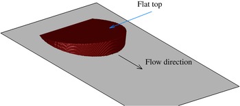
For a finite circular (non-planar/non-two-dimensional) initial release, the presence of the slope changes both the spanwise and streamwise dynamics of the gravity current and makes the large-scale motion of the flow fully three-dimensional. This configuration is of more practical relevance as it has a more similar geometrical configuration to powder snow avalanches and turbidity currents driven by submarine mud slides. A theoretical investigation using the shallow water equations has been conducted by Webber, Jones & Martin (Reference Webber, Jones and Martin1993) who predicted that the gravity current will assume a self-similar circular wedge shape (see figure 1). Tickle (Reference Tickle1996) expanded on the study by Webber et al. (Reference Webber, Jones and Martin1993) to include the effects of entrainment. Ross, Linden & Dalziel (Reference Ross, Linden and Dalziel2002) carried out Boussinesq saline experiments and showed that contrary to the prediction of Webber et al. (Reference Webber, Jones and Martin1993), experimental data show that the gravity current takes on a shape that is more akin to a triangular wedge.
Schematic of the circular wedge from the shallow water model of Webber et al. (Reference Webber, Jones and Martin1993).

In the present investigation, we report data from fully resolved three-dimensional direct numerical simulations of circular, finite-release Boussinesq gravity currents propagating down a uniform slope. Our data show that in most cases, the gravity current evolves to a shape that is more similar to a triangular wedge, as observed in the experiments of Ross et al. (Reference Ross, Linden and Dalziel2002). The physical mechanisms leading to the formation of this triangular shape and the entrainment properties of such a structure will be presented.
Unlike planar (two-dimensional) currents that are always unidirectional (do not admit a mean spanwise component of velocity), or axisymmetric currents that are ever diverging, circular releases on sloping boundaries may exhibit diverging (immediately after release), nearly unidirectional (when the effect of the slope on the spreading current becomes important) or even converging phases (beyond the first acceleration phase in the front velocity) of spreading. Of specific interest is the converging phase of spreading, which leads to local peaks in buoyancy along the centreline of the release, which in turn translates to a second acceleration phase in the front velocity. The details of the second acceleration phase and the redistribution of material leading to its development will be discussed.
These finite-release gravity currents are invariably dominated by the head, where most of the mixing and hence the entrainment of ambient fluid occurs. We present a simple method for defining the head and calculate the various properties pertaining to it, such as the volume, mass, shape, entrainment, Froude number, etc. We find the entrainment coefficient to be nearly independent of the slope, which is in line with previous experimental results. The Froude number in the simulations is observed to slightly increase with steeper slopes, which is consistent with the experimental data.
The remainder of the paper is organized as follows. Previous theoretical and experimental studies on down-slope spreading gravity currents are presented in § 2. In § 3, we outline the numerical set-up and discuss potential discrepancies with the experiments. Results are presented and discussed in the following sections: in § 4 we point out the presence of a second acceleration phase. In §§ 5 and 6 we focus on the head of the gravity current, where a new method for defining the head and extracting its various parameters is highlighted. Finally, conclusions are drawn in § 7.
2 Theory and laboratory experiments
The case of a bottom flowing gravity current on a uniform slope has been investigated in the past. Webber et al. (Reference Webber, Jones and Martin1993) considered the motion of a heavy cloud released on an inclined smooth wall. They found that the two-dimensional shallow water equations admit an analytic solution consisting of a shallow wedge descending at a uniform velocity (figure 1). In their model, the current advances as a coherent structure with a constant width-to-length ratio of
 ${\rm\pi}$
and a height that increases linearly from zero at the current’s back end to its maximum value at the front of the current. At the current–ambient interface, the Froude condition was applied, and the shape was chosen such that the current does not spread in the lateral direction. The wedge does not entrain any ambient fluid and therefore retains its shape as it descends. Webber’s analytic solution neglects internal circulation within the current and thus results in a top surface that remains flat.
Ross et al. (Reference Ross, Linden and Dalziel2002) conducted multiple experiments for bottom spreading gravity currents at slopes ranging from
 $5^{\circ }$
to
 $20^{\circ }$
. Their experiments consisted of releasing a finite volume of relatively dense salty water inside a rectangular tank filled with relatively less dense tap water. The initial density of the current remained below
 $1.03~\text{g}~\text{cm}^{-3}$
(only a few percent larger than that of the ambient tap water), and therefore their experiments may be classified as Boussinesq. In their experiments, they observed the gravity current to take on a shape that is more akin to a triangular wedge, where the majority of the heavy fluid accumulated at the front of the current. Towards the interior and back portions of the current, they observed the formation of a very thin layer of heavy fluid. Their experiments did not agree with the self-similar circular shallow wedge predicted by Webber et al. (Reference Webber, Jones and Martin1993).
3 Direct numerical simulations of circular gravity currents on an incline
3.1 Numerical model
We performed a number of simulations for which a relatively slightly denser fluid confined within a slanted circular cylinder is released on a sloping boundary. We solve the conservation of mass and momentum equations as well as the transport equation for the density field inside a rectangular computational domain. The non-dimensional system of equations reads
 $$\begin{eqnarray}\displaystyle & \displaystyle \boldsymbol{{\rm\nabla}}\boldsymbol{\cdot }\boldsymbol{u}=0, & \displaystyle\end{eqnarray}$$
 $$\begin{eqnarray}\displaystyle & \displaystyle \frac{\text{D}\boldsymbol{u}}{\text{d}t}={\it\rho}\boldsymbol{e}^{g}-\boldsymbol{{\rm\nabla}}p+\frac{1}{Re}{\rm\nabla}^{2}\boldsymbol{u}, & \displaystyle\end{eqnarray}$$
 $$\begin{eqnarray}\displaystyle & \displaystyle \frac{\partial {\it\rho}}{\partial t}+\boldsymbol{{\rm\nabla}}\boldsymbol{\cdot }({\it\rho}\boldsymbol{u})=\frac{1}{Sc\,Re}{\rm\nabla}^{2}{\it\rho}. & \displaystyle\end{eqnarray}$$
 $\boldsymbol{u}$
,
 ${\it\rho}$
and
 $p$
represent the divergence free velocity field, density and pressure, respectively. The density
 ${\it\rho}$
is non-dimensionalized as follows
 $$\begin{eqnarray}{\it\rho}=\frac{{\it\rho}^{\ast }-{\it\rho}_{a}^{\ast }}{{\it\rho}_{c0}^{\ast }-{\it\rho}_{a}^{\ast }}.\end{eqnarray}$$
The asterisk denotes a dimensional quantity, all other quantities are to be taken as non-dimensional. The variables
 ${\it\rho}^{\ast }$
,
 ${\it\rho}_{a}^{\ast }$
and
 ${\it\rho}_{c0}^{\ast }$
represent the local, ambient and initial heavy fluid densities, respectively. Therefore, the value of
 ${\it\rho}$
remains bounded between 0 and 1. The dimensionless pressure is given by
 $$\begin{eqnarray}p=\frac{p^{\ast }}{{\it\rho}_{a}^{\ast }(U^{\ast })^{2}},\end{eqnarray}$$
where
 $p^{\ast }$
and
 $U^{\ast }$
denote the local dimensional pressure and velocity scale, respectively.
 $\boldsymbol{e}^{g}$
is a unit vector pointing in the direction of gravity and the Schmidt,
 $Sc$
, and Reynolds number,
 $Re$
, are defined as
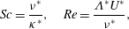 $$\begin{eqnarray}Sc=\frac{{\it\nu}^{\ast }}{{\it\kappa}^{\ast }},\quad Re=\frac{{\it\Lambda}^{\ast }U^{\ast }}{{\it\nu}^{\ast }},\end{eqnarray}$$
where
 ${\it\nu}^{\ast }$
and
 ${\it\kappa}^{\ast }$
represent the kinematic viscosity and molecular diffusivity of the current. We follow Ross et al. (Reference Ross, Linden and Dalziel2002) by defining the length scale
 ${\it\Lambda}^{\ast }$
, the velocity scale
 $U^{\ast }$
and the time scale
 $T^{\ast }$
as
 $$\begin{eqnarray}{\it\Lambda}^{\ast }=(V_{0}^{\ast })^{1/3},\quad U^{\ast }=\sqrt{g^{\ast }\frac{{\it\rho}_{c0}^{\ast }-{\it\rho}_{a}^{\ast }}{{\it\rho}_{a}^{\ast }}{\it\Lambda}^{\ast }},\quad T^{\ast }=\frac{{\it\Lambda}^{\ast }}{U^{\ast }}\end{eqnarray}$$
where
 $V_{0}^{\ast }$
is the initial volume of heavy fluid in the slanted cylinder and
 $g^{\ast }$
denotes the gravitational acceleration.
We implement the Boussinesq approximation of small density difference between the current and the ambient in that the density only appears in the buoyancy term of the momentum equation (first term on the right-hand side of (3.2)). Equations (3.1)–(3.3) are solved using a spectral code (Cortese & Balachandar Reference Cortese and Balachandar1995; Cantero et al.
Reference Cantero, Lee, Balachandar and Garcia2007b
). In the wall-normal,
 $z$
-direction, a no-slip boundary condition is used for the velocity field at the bottom wall and a free-slip boundary condition is used at the top wall, which is parallel to the sloping bottom. Periodic boundary conditions are used for all variables in the streamwise,
 $x$
and spanwise,
 $y$
, directions. This implies that a periodic array of gravity currents is being simulated. Care must be taken to ensure that these currents do not interact as we are interested in the development of an isolated gravity current. The lengths of the domain in the streamwise and spanwise directions are thus chosen to ascertain that there is uninterrupted development of the gravity current. As for the density field, zero gradient conditions are enforced at the top and bottom boundaries. This ensures that there is no density flux across these boundaries.
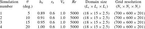
Details of the numerical simulations are described in table 1. The grid resolution was chosen to achieve between 4 and 6 decades of decay in the energy spectra for all variables. It is consistent with the requirement that the grid spacing must be of the order of
 $O(ReSc)^{-1/2}$
(Härtel, Fredrik & Mattias Reference Härtel, Fredrik and Mattias2000; Birman, Martin & Meiburg Reference Birman, Martin and Meiburg2005). Even though the Schmidt number in the experiments of Ross et al. (Reference Ross, Linden and Dalziel2002) has a value of approximately 700 (which is the Schmidt number for salty water), we have used a Schmidt number of unity in all simulations here. Setting the Schmidt number to unity is common practice in simulations (Cantero et al.
Reference Cantero, Lee, Balachandar and Garcia2007b
; Dai Reference Dai2013) to avoid numerical complications. Furthermore, studies conducted by Bonometti & Balachandar (Reference Bonometti and Balachandar2008) have indicated that the resulting flow field is only weakly dependent on Schmidt number provided the Reynolds number of the flow is large. The time step is chosen such that the Courant–Friedrichs–Lewy (CFL) number remains below 0.5. We impose a small random disturbance on the initial density field to stimulate a faster transition to turbulence. The amplitude of the disturbance amounts to 5 % of the density difference between the current and the ambient.
List of simulations. The bottom inclination is denoted by
 ${\it\theta}$
. The mean height, radius and volume of the slanted cylinder are
 $h_{0}$
,
 $r_{0}$
and
 $V_{0}$
, respectively.
 $Re$
represents the Reynolds number. The domain size and the grid resolution are the same for all simulations.
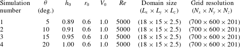
3.2 Effects of domain shape and size
In non-dimensional terms, the length (
 $L_{x}=18$
) and width (
 $L_{y}=15$
) were chosen to correspond to the tank’s dimensions (
 $L_{x}^{exp}\approx 20$
and
 $L_{y}^{exp}\approx 16$
) used in the experiments of Ross et al. (Reference Ross, Linden and Dalziel2002). The main difference between the numerical and experimental set-ups is that the top boundary of the numerical domain is parallel to the slope, whereas in the experiments, the top boundary is horizontal. This means that in the experiments the current flows into a deepening layer of ambient fluid, whereas in the simulations the current flows into an ambient fluid of constant depth. In the experiments, and again in non-dimensional terms, the depth of the ambient fluid increases from approximately 1 at the time of release to approximately 4 in the later stages of the release. This is in contrast to the constant depth of
 $L_{z}=2.5$
in the simulations. Because the ambient water depth in the experiments increases linearly along the streamwise coordinate, the current advances against a mild adverse streamwise pressure gradient. This is in contrast to the zero ambient pressure gradient present in the simulations. The constant streamwise pressure gradient in the experiments is proportional to the slope and is given by
 $$\begin{eqnarray}{\it\Psi}_{a}^{\ast }={{\it\rho}_{a}^{\ast }g}^{\ast }\tan ({\it\theta}),\end{eqnarray}$$
where
 ${\it\theta}$
is the inclination of the bottom wall. From the simulation results we have computed the local streamwise pressure gradient at the front of the current and compared it to
 ${\it\Psi}_{a}^{\ast }$
in order to evaluate the relative importance of the latter. The ratio of
 ${\it\Psi}_{a}^{\ast }$
to the local streamwise hydrostatic pressure gradient in the simulations is simply
 $\tan ({\it\theta})/(\text{d}\bar{h}/\text{d}x)$
, where
 $\bar{h}$
is the
 $z$
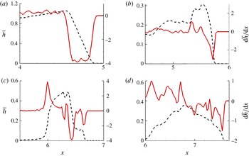
-integrated density field. We plot in figure 2 the variation in
 $\bar{h}$
as well as
 $\text{d}\bar{h}/\text{d}x$
in the symmetry (
 $y=0$
) plane for sim 3 (
 ${\it\theta}=15^{\circ }$
). We observe the magnitude of
 $\text{d}\bar{h}/\text{d}x$
at the front to be approximately 4 at
 $t=0$
. This yields a ratio of
 $\tan ({\it\theta})/(\text{d}\bar{h}/\text{d}x)$
of approximately 0.07. Therefore, at early times, the relative magnitude of the constant hydrostatic pressure gradient due to an increasing ambient depth compared to the hydrostatic pressure gradient at the front is small but not negligible. Similar values are obtained for other slopes.
Vertically integrated density field
 $\bar{h}$
(black dashed line) and
 $\text{d}\bar{h}/\text{d}x$
(solid red line) versus streamwise location
 $x$
in the symmetry (
 $y=0$
) plane at four time instances (
 $t=0$
, 2, 4 and 6) corresponding to (a), (b), (c) and (d), respectively.

Ross et al. (Reference Ross, Linden and Dalziel2002) also carried out surface gravity current experiments to verify whether the fact that the current was spreading on a sloping boundary was more important than the fact that the current was spreading into a deepening layer of fluid. A relatively less dense mixture of fresh water and dye was released into a denser salty water ambient causing the gravity current to spread on the (horizontal) surface of the water. There, the current was only subject to the changing depth of the ambient fluid. Ross et al. (Reference Ross, Linden and Dalziel2002) found no visible difference from the circular spreading shape expected for currents spreading on a bottom horizontal surface. They concluded that the effect of the slope far outweighs the change in ambient depth.
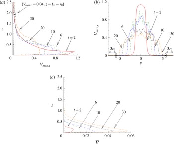
It is important that the depth and width of the numerical domain be large enough such that they do not hinder the spreading of the current. We may test a posteriori whether this is true by inspecting the magnitude of the velocity field as a function of the vertical and spanwise directions. Figure 3(a) shows the maximum fluid velocity magnitude on each plane parallel to the bottom boundary,
 $\max _{xy}(\sqrt{u^{2}+v^{2}+w^{2}})$
, as a function of
 $z$
. It can be seen that the maximum velocity magnitude at a distance of
 $1r_{0}$
from the upper surface remains small, amounting up to only approximately a percent of the velocity scale for the entire duration of the simulation. Figure 3(b) shows the maximum velocity magnitude on a streamwise wall-normal plane (i.e.
 $x$
–
 $z$
plane) as a function of the spanwise direction. From figure 3(b), the spanwise length is large enough to ensure the ambient flow remains stagnant at a distance of over
 $3r_{0}$
from both lateral boundaries. But most importantly, the average streamwise fluid velocity computed on each wall-parallel plane
 $\bar{v}=(1/L_{x}L_{y})\int _{0}^{L_{x}}\int _{0}^{L_{y}}v\,\text{d}x\,\text{d}y$
, is mostly confined to the bottom of the domain, with the peak velocity occurring below
 $z=0.2$
. The bulk flow in the upper half of the domain is practically zero. Unlike in a lock release configuration where there must be a return flow, here the periodic boundary condition along the streamwise direction allows for inflow at the upstream boundary. Any flow in the ambient fluid surely does not extend into the upper half of the domain, where
 $\bar{v}$
is orders of magnitude smaller than in the bottom half. This provides some support to the beliefs that the placement of the upper boundary does not hinder the spreading of the current, and that the effect of the slope remains the overriding factor in these simulations as in the case of the experiments of Ross et al. (Reference Ross, Linden and Dalziel2002). Nevertheless, the effect of the inclined upper surface in the present simulations must be taken into consideration when we present qualitative (in terms of structure and density distribution of the current) and quantitative (specifically for the front position of the current for all slopes considered) comparison with the experiments.
Maximum velocity for simulation 3 in each (a) wall-parallel
 $xy$
-plane and (b) wall-normal
 $xz$
-plane. (c) Average velocity for simulation 3 in each wall-parallel
 $xy$
-plane. See text for definition.

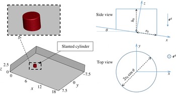
Schematic of the rectangular numerical domain with a side, top and enlarged view of the initial shape of the slanted cylinder containing the heavy fluid.

3.3 Initial conditions
The heavy fluid is initially confined inside a truncated circular cylindrical segment of radius
 $r_{0}\cos {\it\theta}$
and mean height
 $h_{0}$
as shown in figure 4. Here, the angle
 ${\it\theta}$
represents the inclination of the bottom plane with respect to the horizontal along the
 $x$
-axis (there is no inclination along the
 $y$
-axis). The radius and height are measured along the horizontal (normal to the direction of gravity) and vertical (parallel to the direction of gravity) directions, respectively. The shape of the cylinder conforms to that utilized in the experiments of Ross et al. (Reference Ross, Linden and Dalziel2002). From the digitized images of figure 6 in their manuscript, we observe that the lock radius along the inclined plane is held fixed at a non-dimensional value of approximately
 $r_{0}=0.6$
. In their experiments, the cube root of the initial volume of the heavy fluid is taken as a length scale. Consequently, we adopt the same length scale in our simulations and vary the mean height
 $h_{0}$
such that the initial volume of the circular cylindrical segment
 $V_{0}={\rm\pi}(r_{0}\cos {\it\theta})^{2}h_{0}$
is equal to 1, i.e.
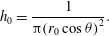 $$\begin{eqnarray}h_{0}=\frac{1}{{\rm\pi}(r_{0}\cos {\it\theta})^{2}}.\end{eqnarray}$$
The values of
 $h_{0}$
for the various slopes are shown in table 1.
4 Results and discussion
4.1 Flow structure
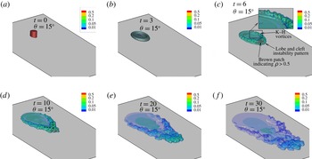
In figure 5, we show multiple semi-transparent isosurfaces of density ranging from
 $0.01\leqslant {\it\rho}\leqslant 0.5$
for a bottom slope of
 ${\it\theta}=15^{\circ }$
. Recall that a non-dimensional density value of
 ${\it\rho}=1$
(
 ${\it\rho}=0$
) corresponds to the current (ambient) density at time of release. The effect of the slope on the gravity current is not immediately perceived. The influence of the slope becomes apparent after some finite time, specifically when the depth-to-length ratio of the current becomes comparable to the gradient of the slope (Ross et al.
Reference Ross, Linden and Dalziel2002). Because of the circular nature of the release, we observe the current to initially spread in an axisymmetric manner, similar to a vortex ring impinging on a wall. Shortly after release (
 $t=3$
), the majority of the heavy fluid accumulates in an outer ring, with a thin layer of fluid residing in the interior of the ring. During those early stages, the current’s front is smooth and nearly axisymmetric.
Snapshots of the current at various times (
 $t=0$
, 3, 6, 10, 20, 30) for a bottom slope
 ${\it\theta}=15^{\circ }$
. The current is visualized with multiple semi-transparent isosurfaces of density with a value of
 ${\it\rho}=(0.01,0.05,0.1,0.2,0.5)$
. Initially, at
 $t=0$
and 3, the current–ambient interface is sharp such that the transition in density from 0.01 to 0.5 occurs over a few grid cells. Because of the sharpness of the interface, the isodensity surfaces are closely packed. The resulting, nearly homogeneous, colour therefore corresponds to a mixture of the 5 chosen isodensity values. At later times (
 $t=6$
and 10), the brown patch at the front of the current corresponds to a region of density in excess of 0.5. Finally, for
 $t\geqslant 20$
, only blue and green colours are present indicating that the maximum density in the current has fallen below 0.2.

At
 $t=6$
, the effect of the inclined boundary is apparent. The current has developed into a boomerang-like structure that progressively thickens (the height of the current increases) as we move closer to the front of the current near the symmetry plane (
 $y=0$
). The thicker current at the downstream end is also due in part to the shape of the release. Recall that the heavy fluid is initially confined within a slanted circular cylinder, and therefore as the inclination of the bottom wall increases, the amount of heavy fluid downstream of the centre of the cylinder increases as well (with respect to the amount of heavy fluid upstream of the centre). The brown colour at the front (downstream end) of the current indicates a relatively denser region compared to its surroundings. We observe multiple undulations at the front of the current corresponding to the lobe and cleft instability pattern (Simpson Reference Simpson1982), a characteristic feature of bottom spreading gravity currents. These undulations are generally observed in the presence of the no-slip boundary condition at the bottom wall (Simpson Reference Simpson1972; Härtel et al.
Reference Härtel, Fredrik and Mattias2000; Cantero et al.
Reference Cantero, Lee, Balachandar and Garcia2007b
). A pattern of rolled up Kelvin–Helmholtz (K–H) vortices is also observed to develop on the sides of the current around
 $t=6$
(see inset for more detail).
At
 $t=10$
, the current is seen to transition to a V-like structure with a vertex angle of
 ${\it\gamma}\approx 85^{\circ }$
. The angle
 ${\it\gamma}$
is observed to decrease at steeper slopes from
 ${\it\gamma}\approx 150^{\circ }$
at
 ${\it\theta}=5^{\circ }$
to
 ${\it\gamma}\approx 80^{\circ }$
at
 ${\it\theta}=20^{\circ }$
(not shown in here). These values of
 ${\it\gamma}$
are all taken at
 $t=10$
. Here
 ${\it\gamma}$
is crudely estimated as the vertex angle between the dashed black lines (figure 5 at
 $t=10$
). The current remains thickest along the centreline (
 $y=0$
plane) towards its downstream end. The height, and consequently the buoyancy, progressively decreases in the upstream direction until it vanishes at the rear end of the current. In the central region, we observe only a thin film of fluid. This is the fluid left over from the initial release after it has been diluted due to mixing with the ambient.
For
 $t\geqslant 20$
bare regions begin to appear behind the front of the gravity current surrounding a thin patch of heavy fluid. These bare regions create an adverse pressure gradient that act to slow down the advancing current. In fact, on a flat bottom these bare regions will result in a reverse flow (Zgheib, Bonometti & Balachandar Reference Zgheib, Bonometti and Balachandar2015).
The structure of the current that we observe in the simulations resembles that in the experiments of Ross et al. (Reference Ross, Linden and Dalziel2002). They observe the majority of the heavy fluid to aggregate near the front (figures 3 and 4 in their manuscript). This increased buoyancy, as discussed later in §§ 4.2 and 4.3, is responsible for a second acceleration in the front velocity of the current. For the
 ${\it\theta}=15^{\circ }$
case, they report the same V-shape structure (figure 3(b) in their manuscript which corresponds to a non-dimensional time of 9) that we detect (
 $t=10$
in figure 5) in our simulations. In both the simulations and experimental data, we do not observe the circular wedge shaped current predicted from the analysis of the shallow water equations by Webber et al. (Reference Webber, Jones and Martin1993).
In the shallow water model, any internal variations in the current’s velocity are not taken into account by the analysis. By assuming a constant velocity (independent of space and time), the height of the current becomes solely a function of the streamwise coordinate (
 $h=h(x)$
). The depth of the current increases linearly in the downstream direction at a rate of (
 $\text{d}h/\text{d}x=\tan {\it\theta}$
). This linear increase results in a circular wedge-like structure for the current with a flat top surface. From the experimental data of Ross et al. (Reference Ross, Linden and Dalziel2002) and the present simulations, the current does not take the form of a wedge-like structure. The centre of the current is always occupied by a thin layer of fluid, and the top surface is observed to be more complex than the predicted flat shape in the shallow water model. The assumption of a constant velocity for the current is not warranted. In fact, internal circulation within the current appears to be important (see figure 6).
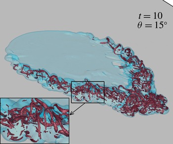
Snapshot of the current at
 $t=10$
for
 ${\it\theta}=15^{\circ }$
. The current is visualized with a semi-transparent isosurface of density with a value of
 ${\it\rho}=0.05$
. The vortical structures in the interior of the current correspond to a swirling strength isosurface of
 ${\it\lambda}_{ci}=4.5$
. Inset: enlarged view showing the hairpin vortical structures.

Figure 6 depicts the vortical structure in the current’s interior for
 ${\it\theta}=15^{\circ }$
(similar structures are observed for the other slopes) at a single instance
 $t=10$
. The current’s surface is visualized through a semi-transparent isosurface of density
 ${\it\rho}=0.05$
. The vortical structures correspond to an isosurface of swirling strength
 ${\it\lambda}_{ci}=4.5$
. The swirling strength
 ${\it\lambda}_{ci}$
represents regions of high vorticity. It is defined as the absolute value of the imaginary part of the complex eigenvalue of the velocity gradient tensor (Zhou et al.
Reference Zhou, Adrian, Balachandar and Kendall1999; Chakraborty, Balachandar & Adrian Reference Chakraborty, Balachandar and Adrian2005). A multitude of hairpin vortices are seen to be aligned along the front of the current (see inset of figure 6). This network of hairpin vortices is responsible for the complex three-dimensional shape observed in figure 5. Furthermore, these vortical structures reveal the importance of internal circulation within the current. Internal circulation is also found in powder-snow avalanches. Turnbull & McElwaine (Reference Turnbull and McElwaine2007) have proposed that the occurrence of the internal flow is one of the main reasons why the shape of the gravity current is sharper than that predicted by Webber et al. (Reference Webber, Jones and Martin1993).
4.2 Front velocity
We first define the current–ambient interface as the position where the wall-normal integrated height of the current
 $\bar{h}(x,y,t)$
exceeds a small threshold value
 ${\it\epsilon}$
. The front position
 $\tilde{x}_{N}(y,t)$
is then taken as the maximum streamwise location of the detected interface. The height of the current
 $\bar{h}$
is defined as
 $$\begin{eqnarray}\bar{h}(x,y,t)=\int _{0}^{L_{z}}{\it\rho}(x,y,z,t)\,\text{d}z.\end{eqnarray}$$
The small threshold value
 ${\it\epsilon}$
is taken to be
 ${\it\epsilon}=10^{-3}$
. The front location is not however sensitive to the chosen value of
 ${\it\epsilon}$
in the range [
 $10^{-4},10^{-2}$
]. To obtain the temporal evolution of the mean front position
 $x_{N}(t)$
, we average the front location
 $\tilde{x}_{N}(y,t)$
over a segment of width
 ${\it\sigma}=0.15$
centred at the symmetry plane (
 $y=0$
).
 $$\begin{eqnarray}x_{N}(t)=\int _{-{\it\sigma}/2}^{{\it\sigma}/2}\tilde{x}_{N}(y,t)\,\text{d}y.\end{eqnarray}$$
The front position,
 $x_{N}(t)$
is not sensitive to the chosen value of
 ${\it\sigma}$
in the range [0.05 0.25].
Alternatively, the height of the current may be defined as the vertical location of the centre of mass
 $$\begin{eqnarray}{\hat{h}}(x,y,t)=\frac{\displaystyle \int _{0}^{L_{z}}{\it\rho}(x,y,z,t)z\,\text{d}z}{\displaystyle \int _{0}^{L_{z}}{\it\rho}(x,y,z,t)\,\text{d}z}.\end{eqnarray}$$
Using
 ${\hat{h}}$
, the front position may be extracted using the inflection point method (Anjum, Mcelwaine & Caulfield Reference Anjum, Mcelwaine and Caulfield2013; Zgheib et al.
Reference Zgheib, Bonometti and Balachandar2015) without a need for specifying a threshold value
 ${\it\epsilon}$
. Because of the relatively sharp current–ambient interface, both the inflection point method and the threshold method give nearly identical results (see inset of figure 7
a).
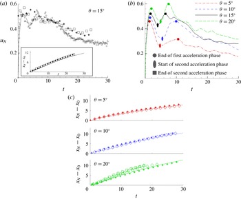
(a) Temporal evolution of the front velocity
 $u_{N}$
for
 ${\it\theta}=15^{\circ }$
from simulation (○) and experiment (
 $+$
▫). The solid line is a smoothing spline fit to the simulation data, and the dashed line is obtained by differentiating a twelfth-order polynomial curve fit to the front location
 $x_{N}$
. (Inset) Travelled distance along the front from simulation (threshold method ——, inflection point method - - -) and experiment (
 $+$
▫). (b) Temporal evolution of the front velocity
 $u_{N}$
for the four slopes (
 ${\it\theta}=5^{\circ },10^{\circ },15^{\circ },20^{\circ }$
) from simulations. The simulation data show a second acceleration phase in the front velocity for all four slopes. (c) Temporal evolution of the front from simulation (lines) and experiment (symbols) for (
 ${\it\theta}=5^{\circ },10^{\circ },20^{\circ }$
).

The temporal evolution of the front from the present simulations is compared to the experimental result of Ross et al. (Reference Ross, Linden and Dalziel2002) in the inset of figure 7(a) for
 ${\it\theta}=15^{\circ }$
, and in frame c for all other slopes. The lines (in frame c and the inset of frame a) represent the simulation data, and the symbols represent digitized experimental data from Ross et al. (Reference Ross, Linden and Dalziel2002). In their experiments, they release a volume of relatively dense saline water into less dense tap water. Their experiments were carried out in a tank of rectangular cross-section with dimensions 2 m
 $\times$
2.5 m (width
 $\times$
length) and an elevation of 0.85 m. The bottom surface of the tank could be adjusted to give a range of slopes between
 $5^{\circ }$
and
 $20^{\circ }$
. A circular slanted cylinder initially contains the salty water mixture, whose density
 ${\it\rho}_{c0}^{\ast }$
never exceeded the tap water density (
 ${\it\rho}_{a}^{\ast }$
) by more than a few per cent. The small density difference in the experiments justifies the use of the Boussinesq model. The initial reduced gravity of the experiments was
 $g_{0}^{\ast \prime }\approx 25~\text{cm}~\text{s}^{-2}$
, and the initial volume of the salty mixture was
 $V_{0}^{\ast }\approx 1800~\text{cm}^{3}$
. The above parameters indicate that the Reynolds number of their experiments was
 $Re\approx 2\times 10^{4}$
. We will discuss the effect of running the simulations at a lower
 $Re$
number in § 6.
Multiple experiments were carried out for each slope, however these only differed slightly (in terms of initial volume and concentration of the saline solution) from one another. The variable
 $x_{0}$
corresponds to the initial location of the front
 $[x_{0}=x_{N}(t=0)]$
, and the difference (
 $x_{N}-x_{0}$
) represents the streamwise distance travelled by the current. We observe good agreement in the front position for all slopes between our simulations and the published experimental data. There are however some significant discrepancies in the front velocity, namely the absence of a second acceleration phase in the experiments, as well as differences in the later stages (
 $t>15$
) for
 ${\it\theta}=15^{\circ }$
. The reason for these differences remains somewhat unclear for the moment, and perhaps may be attributed to differences between the experimental and computational set-ups discussed in § 3.2. The front velocity however compares reasonably at late times for the majority of the other experiments (
 ${\it\theta}=5^{\circ },10^{\circ },20^{\circ }$
).
The front velocity
 $u_{N}$
is obtained by differentiating the front location with respect to time using a second-order central finite difference scheme. Figure 7(a) shows the temporal evolution of the front velocity
 $u_{N}(t)$
for
 ${\it\theta}=15^{\circ }$
. The experimental data (square and plus sign symbols) are not directly obtained from Ross et al. (Reference Ross, Linden and Dalziel2002) since they do not explicitly report the front velocity in their manuscript. They are obtained from differentiating the front location recovered from the digitized images of the temporal evolution of the front (symbols in the inset of figure 7
a). It should be noted however, that Ross et al. (Reference Ross, Linden and Dalziel2002) do calculate the front velocity as it is needed to derive other quantities such as the Froude number. We can see, from figure 7(a) that the front speed
 $u_{N}(t)$
is not very sensitive to the method by which it is calculated.
Figure 7(b) shows the temporal evolution of the front velocity for the four slopes (
 ${\it\theta}=5^{\circ },10^{\circ },15^{\circ },20^{\circ }$
). It reveals some very interesting dynamics that has not been reported for finite-release gravity currents on a sloping boundary. Unlike axisymmetric gravity currents that spread on a horizontal flat surface, in these downhill spreading currents the initially circular finite releases are seen to undergo a second acceleration phase immediately following the first acceleration phase. At the end of the first acceleration phase, the current attains, for the majority of the slopes (excluding
 ${\it\theta}=20^{\circ }$
), its maximum velocity. We observe the maximum velocity at the end of the first acceleration phase to monotonically increase with steeper slopes from
 $u_{N}\approx 0.46$
when
 ${\it\theta}=5^{\circ }$
to
 $u_{N}\approx 0.56$
when
 ${\it\theta}=20^{\circ }$
. We also observe the time it takes the current to reach this first local maximum value to monotonically increase with slope angle
 ${\it\theta}$
as well from
 $t\approx 1.4$
when
 ${\it\theta}=5^{\circ }$
to
 $t\approx 2$
when
 ${\it\theta}=20^{\circ }$
.
The current then decelerates to a local minimum. Interestingly enough, at the end of the first acceleration phase, the current redistributes itself (in such a way as to increase the buoyancy at the centreline) and undergoes a second acceleration phase to propel the front velocity to a second local maximum, whose value ranges approximately from 70 to 107 % (of the maximum value at the end of the first acceleration phase) for slopes of
 $5^{\circ }$
and
 $20^{\circ }$
, respectively. The rate at which the front velocity transitions from its local minimum to the second maximum is observed to increase with increasing slope. Furthermore, the time it takes the current to undergo such a transition is seen to decrease with steeper slopes from
 ${\rm\Delta}t\approx 5.7$
(
 ${\it\theta}=5^{\circ }$
) to
 ${\rm\Delta}t\approx 2.6$
(
 ${\it\theta}=20^{\circ }$
).
At the end of the second acceleration phase (second maximum in front velocity), the front velocity from the simulations and that obtained from differentiating the front location of the digitized images of Ross et al. (Reference Ross, Linden and Dalziel2002) experiments are in reasonable agreement for the majority of the experiments (shown for the case of
 ${\it\theta}=15^{\circ }$
in figure 7
a). We should note however the discrepancy for sim 3 (
 ${\it\theta}=15^{\circ }$
) at late times (
 $t>15$
) and the absence of the second acceleration in the experiments. We do however observe, in the simulations just as in the experiments, the V-like structure and preferential density distribution (near the centre of the current) shortly after the second acceleration.
The second acceleration phase is in itself interesting from a fluid mechanics point of view, but it also has a long term effect on the current. The second acceleration phase significantly raises the front velocity in a relatively short period of time (especially at steeper slopes), which allows the current’s speed to asymptote to a larger value at later times. This could have implications in problems such as snow avalanches (see study by Turnbull & McElwaine (Reference Turnbull and McElwaine2007)), where neglecting the second acceleration phase could underpredict the velocity, extent, erosive power as well as the destructive capabilities of the avalanche.
The presence of the second acceleration phase indicates a rearrangement or redistribution of the heavy material within the current to increase the buoyancy at the downstream end of the current near the centreline (
 $y=0$
plane). Unlike planar, two-dimensional gravity currents (which are unidirectional whether advancing on a sloping or horizontal boundary), or cylindrical, axisymmetric currents on horizontal boundaries which are ever diverging (as they continually expand radially outwards), circular currents on sloping boundaries will initially advance in a diverging manner (similar to the spreading on horizontal boundaries) and later seem to reorient themselves in such a way so as to converge towards the centreline (during a finite time span). This convergence of material towards the centreline is the primary cause for the second acceleration phase. This mechanism will be explored in more detail in the next sections.
(a) Spanwise (
 $\bar{h}_{y}$
) and (b) streamwise (
 $\bar{h}_{x}$
) averages of the mean height (
 $\bar{h}$
) at
 $t=0$
, 3, 6, 10, 20, 30 for
 ${\it\theta}=15^{\circ }$
.
 $\bar{h}_{x}$
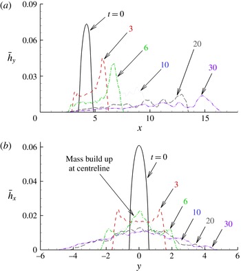
reveals a mass build up near the centreline. (a) Can be thought of as a side view. (b) Can be thought of as a front view.

4.3 Mass redistribution
4.3.1 Spanwise and streamwise average
In order to better understand how the material within the current redistributes itself at the various stages of spreading, we investigate the spanwise and streamwise averages of the vertically integrated density field of the current
 $\bar{h}(x,y,t)$
defined previously in (3.9). We denote by
 $\bar{h}_{x}(y,t)$
and
 $\bar{h}_{y}(x,t)$
the streamwise and spanwise averages of
 $\bar{h}(x,y,t)$
, respectively:
 $$\begin{eqnarray}\displaystyle \bar{h}_{x}(y,t)=\frac{1}{L_{x}}\int _{0}^{L_{x}}\bar{h}(x,y,t)\,\text{d}x, & & \displaystyle\end{eqnarray}$$
 $$\begin{eqnarray}\displaystyle \bar{h}_{y}(x,t)=\frac{1}{L_{y}}\int _{-L_{y}/2}^{L_{y}/2}\bar{h}(x,y,t)\,\text{d}y. & & \displaystyle\end{eqnarray}$$
 ${\it\theta}=15^{\circ }$
. Firstly, from
 $\bar{h}_{x}(y,t)$
, we observe the current to retain its symmetry about the centreline plane (
 $y=0$
) for the whole duration of the simulation.
At
 $t=3$
, the streamwise mass average, (
 $\bar{h}_{x}$
) is very similar for all slopes (not shown here). For
 ${\it\theta}=15^{\circ }$
, we notice the mass to be uniformly distributed in the central region (
 $-1\leqslant y\leqslant 1$
) with a symmetric double peak at
 $y=\pm 1.5$
before a sharp decline to a zero value. Furthermore, from the spanwise mass average (
 $\bar{h}_{y}$
), we observe the majority of the heavy fluid to aggregate in the downstream end of the current as a consequence of the sloping boundary.
At
 $t=6$
, the distribution of
 $\bar{h}_{x}$
reveals a build up of mass near the centreline as indicated by the central peak at
 $y=0$
. In fact
 $\bar{h}_{x}$
at
 $y=0$
at
 $t=6$
is larger than the value at
 $t=3$
, clearly indicating convergence of mass towards the centreline. The mass build up is intensified for larger slopes becoming easily identifiable at
 ${\it\theta}=15^{\circ }$
(figure 8
b) and
 ${\it\theta}=20^{\circ }$
(not shown here). Furthermore, with respect to the spanwise average, we observe the heavy material to continue to aggregate near the downstream end of the current. The mass build up and the preferential accumulation of heavy material at the downstream end increase the buoyancy in the foremost centreline region of the current and subsequently result in the aforementioned second acceleration phase in the front velocity. The time for which the mass build up is perceived (
 $3\lesssim t\lesssim 6$
) is in line with the initiation of the second acceleration phase (
 $t\approx 4$
in figure 7
a).
4.3.2 Instantaneous velocity field
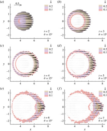
The density weighted, vertically averaged streamwise and spanwise components of velocity provide a good indication of the instantaneous redistribution of the heavy fluid. The components of the instantaneous vector field are defined as
 $$\begin{eqnarray}\displaystyle \text{streamwise component}\quad \bar{u}_{{\it\rho}}(x,y,t)=\frac{\displaystyle \int _{0}^{L_{z}}{\it\rho}u\,\text{d}z}{\displaystyle \int _{0}^{L_{z}}{\it\rho}\,\text{d}z}, & & \displaystyle\end{eqnarray}$$
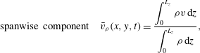 $$\begin{eqnarray}\displaystyle \text{spanwise component}\quad \bar{v}_{{\it\rho}}(x,y,t)=\frac{\displaystyle \int _{0}^{L_{z}}{\it\rho}v\,\text{d}z}{\displaystyle \int _{0}^{L_{z}}{\it\rho}\,\text{d}z}, & & \displaystyle\end{eqnarray}$$
 $u(x,y,z,t)$
and
 $v(x,y,z,t)$
are the streamwise and spanwise components of the three-dimensional velocity field
 $\boldsymbol{u}(x,y,z,t)$
, respectively. The instantaneous vector field multiplied by the vertically averaged height
 $\bar{h}(x,y,t)$
is shown in figure 9. The vectors overlay isocontours of
 $\bar{h}$
to clearly identify the location of the current with respect to the velocity field. A reference vector of 0.5 magnitude is shown in the upper left corner for
 $t=2$
, and the same vector length scale is utilized for all instances.
Instantaneous vector field derived from the density weighted, vertically averaged streamwise and spanwise components of velocity. The vector field overlays isocontours of the vertically integrated current height
 $\bar{h}$
.

The current’s initial velocity (
 $t=2$
and
 $t=3$
) may be split into two components. The first component corresponds to a radially outward diverging flow away from the centre of mass due to the circular shape of the release. The second component is parallel to the
 $x$
-axis and is due to the presence of the slope. At
 $t=4$
and
 $t=5$
, just around the time the second acceleration begins to take effect (
 $t\approx 4$
in figure 7
a), we observe the heavy fluid in the head of the current to converge towards the symmetry plane (
 $y=0$
). Shortly thereafter, at
 $t\geqslant 6$
, the current reorients itself to flow in the streamwise
 $x$
-direction.
This converging flow is observed for the four bottom inclinations (
 ${\it\theta}=5^{\circ },10^{\circ },15^{\circ },20^{\circ }$
), however at various degrees of intensity and over different periods of time. The shallower the slope the weaker the flux of heavy fluid towards the centreline, and the longer the duration of the converging state. On the other hand, for steeper slopes, the concentration of heavy fluid towards the centreline is more powerful and occurs over a shorter period of time. The stronger flux of heavy fluid (towards the symmetry
 $y=0$
-plane) during this period conforms to the faster rate (with respect to the shallower slopes) at which the front moves forward during the second acceleration phase and transitions from a local minimum to a local maximum in the front velocity (figure 7
b). Also from figure 9(a,b), the time evolution of the shape of the current becomes clear. The current takes on a boomerang-like shape at around
 $t=5$
and then evolves to take on a sharper V-shaped front. The angle of the V-shaped front may be crudely estimated as the vertex angle of a wedge (figure 9
c,d). The wedge is chosen such that each leg bisects the thickness of the current in the streamwise direction. The vertex angle is found to be
 ${\it\gamma}=150^{\circ }$
(
 ${\it\gamma}=130^{\circ }$
) for
 $t=6$
(
 $t=7$
).
4.4 Underlying mechanism for converging flow
We presented evidence for the converging flow in the previous sections, and here we will briefly discuss a possible explanation for this phenomenon. For the flow to converge towards the centreline, a region of relatively low pressure is needed in the head of the current (specifically near the centreline) to draw the heavy fluid inwards. Clearly, the pressure and the amplitude of the local flow velocity are related by Bernoulli’s equation.
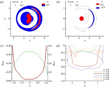
(a,b) Contours of amplitude of the flow velocity
 $q$
and total pressure
 $p$
in the wall-parallel
 $z=0.25$
-plane at
 $t=2$
for
 ${\it\theta}=15^{\circ }$
. The black thin line represents the location of the current and corresponds to an isovalue of
 ${\it\rho}=0.2$
. (c) Minimum total pressure,
 $p_{min}$
, (solid line) and maximum velocity amplitude,
 $q_{max}$
, (dashed line) in the streamwise direction (taken from frames a and b) as a function of spanwise location. (d) Minimum total pressure,
 $p_{min}$
, in the wall-parallel
 $z=0.25$
-plane at multiple times for
 ${\it\theta}=15^{\circ }$
.

Shortly after release (
 $t=2$
), the amplitude of the three-dimensional velocity field,
 $q=\sqrt{u^{2}+v^{2}+w^{2}}$
, in the head of the current attains a maximum value at the centreline and monotonically decreases as we move away from the symmetry
 $y=0$
-plane (figure 10). This non-uniform velocity profile results from (i) the azimuthally dependent (with respect the vertical axis of the cylinder) initial distribution of heavy fluid within the cylinder and (ii) the axisymmetric-like initial spreading coupled with the forcing in the downstream direction (due to the bottom slope). As seen in figure 10, this non-uniform velocity field produces a pressure profile consistent with the pressure field needed to achieve a converging flow towards the centreline. Similar pressure profiles are observed up to
 $t=3$
(in figure 10
d) before the apparent converging flow at
 $t=4$
in figure 9. We observe a different trend at
 $t=4$
in the pressure field, where the pressure at the centreline is largest. This adverse pressure gradient will act to slow the converging flow. Finally by
 $t=6$
, we no longer observe a clear trend in the pressure field. This is consistent with the nearly unidirectional flow along the streamwise direction observed at late times (
 $t=7$
) in figure 9. Furthermore, the larger the bottom slope, the more prominent the variation in the velocity field along the front of the current and the stronger the intensity of the converging flow and consequently the amplitude of the second acceleration. This is again consistent with the intensity of the converging flow and the amplitude of the second acceleration observed for the range of slopes considered,
 ${\it\theta}=5^{\circ },10^{\circ },15^{\circ }$
and
 $20^{\circ }$
.
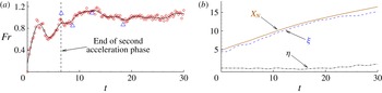
(a) Temporal evolution of the Froude number for
 ${\it\theta}=15^{\circ }$
. The circles correspond to the present simulation data. The solid black line is a third-order smoothing spline to help guide the eyes. The triangles correspond to experimental data from Ross et al. (Reference Ross, Linden and Dalziel2002). The vertical dashed line marks the end of the second acceleration phase. (b) The front position is denoted by
 $x_{N}$
;
 ${\it\xi}(t)$
and
 ${\it\eta}(t)$
represent the streamwise and spanwise coordinates of the position of the maximum height
 $\bar{h}_{Max}$
(used for calculating the Froude number), respectively.

5 Head and entrainment
5.1 Front Froude number
The Froude number of a gravity current relates the front speed
 $u_{N}$
to the nose height
 $h_{N}$
. Here, we calculate the Froude number by using the maximum height
 $\bar{h}_{Max}$
, defined as the maximum value of
 $\bar{h}(x,y,t)$
in the domain. The Froude number is defined as
 $$\begin{eqnarray}Fr=\frac{u_{N}}{(\bar{h}_{Max})^{1/2}}.\end{eqnarray}$$
Figure 11(a) shows the temporal evolution of the Froude number for
 ${\it\theta}=15^{\circ }$
. The circular hollow symbols represent the Froude number as calculated from (5.1), and the solid line is a third-order cubic smoothing spline through the circular hollow symbols to help guide the eyes. The triangular symbols are from the experimental data of Ross et al. (Reference Ross, Linden and Dalziel2002). It should be noted that, in the experiments,
 $\bar{h}_{Max}$
in (5.1) is computed as the product of the height of the front by the maximum reduced gravity. These quantities are inferred from conductivity probe measurements at a discrete set of points, and therefore entail some unavoidable uncertainty. Nonetheless, because the fluid in the head is well mixed, the maximum and mean values of the reduced gravity are statistically similar as can be seen in figure 12. The streamwise (
 ${\it\xi}$
) and spanwise (
 ${\it\eta}$
) coordinates of the position of the maximum height
 $\bar{h}_{Max}$
are shown in figure 11(b). We observe
 $\bar{h}_{Max}$
to be located slightly behind the front of the current at close proximity to the centreline (
 $y=0$
). The vertical dashed line in figure 11(a) marks the time for which the current attains its maximum velocity at the end of the second acceleration phase. Our simulation results are in reasonable agreement with the experimental data of Ross et al. (Reference Ross, Linden and Dalziel2002) for all four slopes (only the results for
 ${\it\theta}=15^{\circ }$
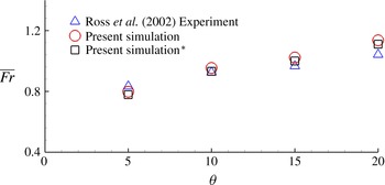
are shown here). Beyond the second acceleration phase, we observe the Froude number to attain a nearly constant value, which appears to increase with steeper slopes (figure 12). Figure 12 shows the dependence of the mean Froude number
 $\overline{Fr}$
on the bottom inclination angle
 ${\it\theta}$
, beyond the second acceleration phase. The mean Froude number is defined as
 $$\begin{eqnarray}\bar{Fr}=\frac{1}{t_{f}-t_{s}}\int _{t_{s}}^{t_{f}}Fr(t)\,\text{d}t,\end{eqnarray}$$
where
 $t_{s}$
and
 $t_{f}$
represent the non-dimensional times that mark the end of the second acceleration phase (second local maximum) and the end of the simulations (
 $t=30$
), respectively. The triangular symbols in figure 12 represent the average value of the Froude number from the Ross et al. (Reference Ross, Linden and Dalziel2002) experiments. The average is taken over the same time interval as in the simulations. The mean Froude number from experiments and simulations are in good agreement. Both are seen to increase with increasing slopes from a value of approximately 0.8 to 1.2 at
 ${\it\theta}=5^{\circ }$
to
 $20^{\circ }$
, respectively.
Mean Froude number as a function of bottom inclination from the present simulation (○ and ▫) and Ross et al. (Reference Ross, Linden and Dalziel2002) experiment (
 ${\rm\Delta}$
). The circles correspond to the mean as computed from (5.1) with
 $\bar{h}_{Max}(t)=\max [\bar{h}(x,y,t)]$
, whereas for the squares,
 $\bar{h}_{Max}(t)$
is computed in the same manner as in the experiments of Ross et al. (Reference Ross, Linden and Dalziel2002). Experiment and simulation are in good agreement. Froude number is observed to increase linearly with bottom slope. This trend is only valid for the considered range and might not continue for much larger slopes.

Gravity currents from finite releases are known to take the shape of a slug with an elevated head and a relatively thin trailing body (Cantero et al. Reference Cantero, Lee, Balachandar and Garcia2007b ; Dai et al. Reference Dai, Ozdemir, Cantero and Balachandar2012). These finite-release currents are invariably dominated by the head, which are generally more turbulent and energetic compared to the trailing body. Most studies consider entrainment of ambient fluid into the current to occur mostly in the head (Beghin et al. Reference Beghin, Hopfinger and Britter1981; Ross et al. Reference Ross, Linden and Dalziel2002; Maxworthy Reference Maxworthy2010). The definition of what constitutes the head of a gravity current is somewhat ambiguous as there is no clear mathematical expression for defining the shape of the head. In the case of planar currents, the shape of the head is inferred from the width and depth-averaged density field of the current. For these canonical geometries, it is relatively easy to identify the head of the current (Dai Reference Dai2013). In what follows we will quantify the head in the present simulations.
5.2 Properties of the head
5.2.1 Defining the head of the gravity current
The present configuration is neither planar nor axisymmetric, and defining the head of the current is more challenging than for canonical set-ups. In essence, a robust method should provide a three-dimensional indicator function
 $I(x,y,z,t)$
defined as
 $$\begin{eqnarray}\displaystyle I(x,y,z,t)=\left\{\begin{array}{@{}ll@{}}1 & \text{in the head of the current}\\ 0 & \text{elsewhwere}.\end{array}\right. & & \displaystyle\end{eqnarray}$$
In the present study, we propose a simple method by which we define the indicator function
 $I$
. The method consists of two steps. First we determine the shape of the current by choosing a threshold isosurface of density (
 ${\it\rho}={\it\rho}_{th}$
). The height of the current
 $h(x,y,t)$
at every point on the
 $x$
–
 $y$
plane simply becomes the vertical distance from the bottom wall to this isosurface. Second we define the head of the current as the envelope of location on the
 $x$
–
 $y$
plane where the height
 $h$
exceeds a threshold value
 $h_{th}$
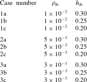
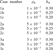
. Table 2 shows the different combinations of
 ${\it\rho}_{th}$
and
 $h_{th}$
considered in this study. Three values of
 ${\it\rho}_{th}$
were examined,
 ${\it\rho}_{th}=10^{-2}$
,
 $5\times 10^{-3}$
and
 $3\times 10^{-3}$
. For each of the isosurface values, we considered three height thresholds
 $h_{th}=0.3$
, 0.25 and 0.2. Out of the 9 possible combinations, we chose case
 $1a$
(table 2) which corresponds to
 ${\it\rho}_{th}=10^{-2}$
and
 $h_{th}=0.3$
. But the conclusions to be drawn are independent of this precise choice.
Parameters used for defining the head.
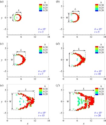
A wall-normal view of the head, obtained using the threshold
 $1a$
in table 2, is depicted in figure 13. We show the evolution of the head at 6 select instances, namely
 $t=3$
, 5, 7, 10, 15 and 20. The red, green and cyan colours represent thresholds
 $1a$
,
 $1b$
and
 $1c$
, respectively. Employing the parameters from threshold
 $1a$
(red colour), we observe the shape of the head to conform to the three-dimensional structure of the current in figure 5. The different shapes the head attains (circular, boomerang, V-shape) as it evolves in time are well captured. Moreover, the thin layer of fluid in figure 5 does not fall under the chosen threshold criterion and is therefore excluded from the head. The total buoyancy in the domain is conserved, but the shape of the head continues to grow with time due to entrainment of ambient fluid.


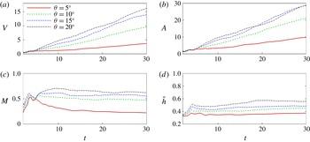
Temporal evolution of the volume
 $V$
, mass
 $M$
, wall-normal projected area
 $A$
, mean height of the head
 $\tilde{h}$
.

Parameters and derived quantities pertaining to the head of the gravity current.

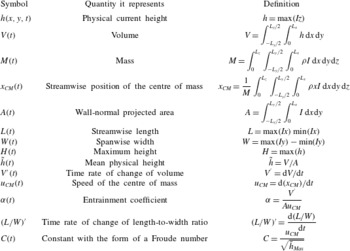
Once the head is defined, its properties (volume, mass, position of the centre of mass, etc.) and other derived quantities (time rate of change of volume, time rate of change of mass, speed of the centre of mass) may be easily extracted. Table 3 lists the various properties and derived quantities pertaining to the head.
5.2.2 Geometric properties and total buoyancy
Figure 14 depicts the temporal evolution of the volume
 $V$
, mass
 $M$
, wall-normal projected area
 $A$
and mean height of the head
 $\tilde{h}$
. We should keep in mind that these quantities are representative of the head, and therefore they are only meaningful after the head has formed. Because the head needs a finite time to develop (approximately
 $2$
time units in the present case), we only need to monitor and investigate these quantities in a time range from
 $t=2$
onwards.
The volume of the head continues to increase with time due to entrainment of ambient fluid. The mean time rate of change (
 $\bar{V^{\prime }}$
) is observed to increase with the slope from a value of
 $\bar{V^{\prime }}\approx 0.1$
at (
 ${\it\theta}=5^{\circ }$
) to
 $\bar{V^{\prime }}\approx 0.55$
at (
 ${\it\theta}=20^{\circ }$
). Here
 $\bar{V^{\prime }}$
represents the average time rate of change from
 $t=10$
to 30. The area
 $A$
is seen to increase at roughly the same rate as the volume, whereas the mean height of the head,
 $\tilde{h}$
, is observed to first increase linearly between
 $t=2$
and 4, and then quickly asymptote to a constant value. The rate at which the mean height increases and the value to which it asymptotes are observed to depend on the slope (the rate being faster and the value of the asymptote being larger for steeper slopes). The volume is therefore growing more as a result of streamwise and spanwise expansion in the plan area of the head, and less because of the head increasing in mean height. This is consistent with previously published results on downhill spreading planar gravity currents (Dai Reference Dai2013). Dai (Reference Dai2013) observed the length and height of the head to initially increase at a rate which depended on the slope angle. He then observed the length to continue to increase at a much larger rate than the height. It is interesting to note that the effect of entrainment is to increase the mean height of the head,
 $\tilde{h}$
, which represents the physical dimension of the current head (see definition in table 3). It is not to be confused with
 $\bar{h}$
(the vertical integral of the density) defined previously in (4.1). This is opposed by gravity, which acts to stratify the medium and push the heavy fluid downwards. The slowly varying mean height beyond
 $t=10$
suggests that these forces are in near equilibrium. Furthermore, the component of gravity in the wall-normal direction decreases with increasing slope, which provides reasoning for the larger mean height at larger slopes. As for the mass in the head, it decreases at a slow rate beyond
 $t\approx 10$
, where it makes up approximately one-fourth of the initial released mass for
 ${\it\theta}=5^{\circ }$
and approximately 50 to 60 % of the initial mass for the steeper slopes,
 ${\it\theta}=10^{\circ },15^{\circ }$
and
 $20^{\circ }$
.
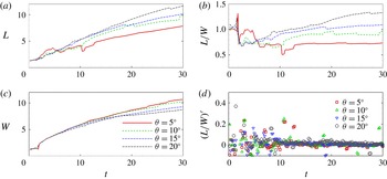
Figure 15 shows the length (
 $L$
), width (
 $W$
), their ratio (
 $L/W$
) and its time rate of change
 $(L/W)^{\prime }$
in the head of the current. We observe both the length and the width to continue to increase with time. Their ratio (
 $L/W$
), however increases at a much slower rate beyond the second acceleration phase (figure 15
d) and seems to depend on the slope angle,
 ${\it\theta}$
(being larger for larger slopes). Beyond
 $t\approx 15$
, the time rate of change of (
 $L/W$
) is small (
 $L/W<0.05$
) and the current attains a self-similar form. This is in line with the three-dimensional structure of the current shown in figure 7, where similar profiles are detected for
 $t=20$
and
 $t=30$
.
Length (
 $L$
), width (
 $W$
), length-to-width ratio (
 $L/W$
) and the time rate of change of the length-to-width ratio
 $(L/W)^{\prime }$
as function of time for
 ${\it\theta}=5^{\circ }$
,
 $10^{\circ }$
,
 $15^{\circ }$
and
 $20^{\circ }$
.

5.2.3 Comparisons with thermal theory and experiments
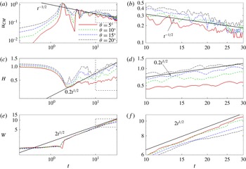
In the present section we test some of the properties of the head of the gravity current against those adopted for thermal theory developed for free axisymmetric vertical thermals. Turner (Reference Turner1973) shows the horizontal radius (or extent) of a thermal and the speed of the cap of the thermal to scale as
 $$\begin{eqnarray}\displaystyle \left.\begin{array}{@{}c@{}}\hat{r}\propto t^{1/2},\\ {\hat{w}}\propto t^{-1/2}.\end{array}\right\} & & \displaystyle\end{eqnarray}$$
In our notation (table 3), the horizontal radius
 $\hat{r}$
would represent the maximum height (
 $H$
) or the maximum width (
 $W$
) of the head, and the speed of the cap of the thermal (
 ${\hat{w}}$
) is synonymous to the speed of the centre of mass (
 $u_{CM}$
).
Log–log plots of (a) the speed of the centre of mass (
 $u_{CM}$
), (c) maximum height (
 $H$
) and (e) maximum width (
 $W$
) in the head as function of time for
 ${\it\theta}=5^{\circ }$
,
 $10^{\circ }$
,
 $15^{\circ }$
and
 $20^{\circ }$
. An enlarged view corresponding to the dashed rectangle is shown on the right-hand side (b,d,f).

Figure 16 shows the log–log plots of the temporal evolution of
 $u_{CM}$
,
 $H$
and
 $W$
for slopes
 ${\it\theta}=5^{\circ }$
,
 $10^{\circ }$
,
 $15^{\circ }$
and
 $20^{\circ }$
. A zoomed in view for
 $t\geqslant 10$
is shown on the right-hand side of each figure. Also shown in the figure are solid black lines that correspond to
 $t^{-1/2}$
(
 $u_{CM}$
),
 $0.22t^{1/2}$
(
 $H$
) and
 $2t^{1/2}$
(
 $W$
), as indicated in the scaling relationships in (5.4) and they are plotted for
 $t\geqslant 10$
and
 ${\it\theta}\geqslant 10^{\circ }$
. The comparison is only qualitative due to the large oscillations in the computed values and also due to the limited time interval of comparison. It should be noted however that even though
 $H$
and
 $W$
both increase as the square root of time, the width is observed to increase at an order of magnitude faster rate. This is because in the present set-up, gravity acts to oppose any increase in the height but does not directly affect growth in the width of the current. For the height to increase, the current must entrain light, ambient fluid from the top, which means that its centre of mass must rise (leading to an increase in the potential energy of the current).
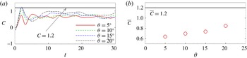
The quantity
 $C$
(table 3), which has the form of a Froude number, is shown in figure 17(a). The value of
 $C$
in our simulations remains constant beyond
 $t\approx 10$
, and its mean value,
 $\bar{C}$
(beyond
 $t=10$
), is shown to depend on the inclination angle
 ${\it\theta}$
. It increases from
 $\bar{C}\approx 0.6$
at
 ${\it\theta}=5^{\circ }$
to
 $\bar{C}\approx 0.9$
at
 ${\it\theta}=20^{\circ }$
. A constant value of
 $C$
is usually observed in experiments (Turner Reference Turner1973), however reported values may differ significantly from one experiment to the other. For vertical spreading thermals, a mean value of
 $C=1.2$
is reported (Turner Reference Turner1973). It is tempting to conjecture that the increase in
 $\bar{C}$
observed in the simulation could continue to larger values as
 ${\it\theta}\rightarrow 90^{\circ }$
. However, it should be noted that rising thermals are axisymmetric, whereas the sloping plane offers only a plane of symmetry.
(a) Temporal evolution of
 $C$
. (b) Mean value of
 $C$
as a function of bottom slope
 ${\it\theta}$
.

The entrainment of ambient fluid occurs primarily in the head of the gravity current (Beghin et al.
Reference Beghin, Hopfinger and Britter1981; Ross et al.
Reference Ross, Linden and Dalziel2002). It is the region where most of the heavy fluid accumulates and the majority of mixing occurs as a result of the head being much more energetic than the thin trailing body. The entrainment coefficient
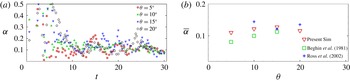
 ${\it\alpha}$
(defined in table 3) is shown in figure 18 at the various slopes (
 ${\it\theta}=5^{\circ },10^{\circ },15^{\circ }$
and
 $20^{\circ }$
). Beyond the second acceleration phase, the value of
 ${\it\alpha}$
does not appear to be significantly influenced by the slope (similar observations were reported by Ross et al. (Reference Ross, Linden and Dalziel2002). Average values (
 $\bar{{\it\alpha}}$
) beyond
 $t=10$
compare favourably with previous experiments and theoretical models, where the entrainment coefficient is found to be of the order of 0.1 (Turner Reference Turner1973; Beghin et al.
Reference Beghin, Hopfinger and Britter1981; Ross et al.
Reference Ross, Linden and Dalziel2002). The square symbols in figure 18(b) are from the experiments of Beghin et al. (Reference Beghin, Hopfinger and Britter1981) in which they investigate the release of a planar current on a sloping boundary. The plus symbols are from the integral model of Ross et al. (Reference Ross, Linden and Dalziel2002).
(a) Temporal evolution of the entrainment coefficient
 ${\it\alpha}$
. (b) Mean value of
 ${\it\alpha}$
beyond
 $t=10$
as a function of bottom slope
 ${\it\theta}$
.

6 Reynolds number effect
The Reynolds number (as defined in (3.6a,b
)) of the lock release experiments of Ross et al. (Reference Ross, Linden and Dalziel2002) is of the order of
 $20\,000$
, whereas our simulation
 $Re$
is approximately four times lower
 $Re=5000$
. As mentioned earlier in § 3.1, the grid spacing for direct numerical simulations of lock release gravity currents must be of the order of
 $O(ReSc)^{-1/2}$
(Härtel et al.
Reference Härtel, Fredrik and Mattias2000; Birman et al.
Reference Birman, Martin and Meiburg2005). Therefore, if we were to simulate the same problem with the same domain size at the larger
 $Re=20\,000$
value, we would need approximately twice as many grid points in each direction for a total of 8 times more grid points in the full numerical domain. In addition to the finer resolution, the time step must be also reduced to temporally resolve the small-scale structures and comply with the CFL condition. At least a 50 % reduction in the time step is necessary to maintain the same CFL number as in the lower
 $Re$
-simulations. Therefore a simulation that takes approximately 3 weeks using 32 processors at
 $Re=5000$
can take up to a year to finish for
 $Re=20\,000$
(using the same number of processors).
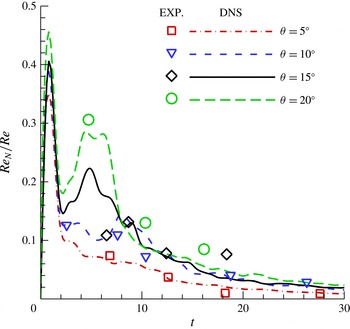
Normalized front Reynolds number (
 $Re_{N}/Re$
) versus time from simulation (lines) and experiment (symbols) for the four bottom inclinations
 ${\it\theta}=5^{\circ }$
,
 $10^{\circ }$
,
 $15^{\circ }$
and
 $20^{\circ }$
.

Even though the
 $Re$
number of our simulations is four times lower than in the experiments, once the flow develops, the ratio of the local Reynolds number of the front (
 $Re_{N}$
) to the Reynolds number (
 $Re$
)
 $$\begin{eqnarray}\frac{Re_{N}}{Re}=u_{N}(\bar{h}_{Max})^{1/2},\end{eqnarray}$$
becomes comparable to those in the experiments. Here
 $Re_{N}(t)$
is based on the front velocity
 $u_{N}$
and the maximum height in the domain
 $\bar{h}_{Max}$
. Figure 19 shows the temporal evolution of the normalized front Reynolds number (
 $Re_{N}/Re$
) from experiments (Ross et al.
Reference Ross, Linden and Dalziel2002) and simulations. Here
 $Re_{N}$
is only meaningful from
 $t=2$
onwards, after the head of the current has formed and when
 $\bar{h}_{Max}$
corresponds to the maximum height in the head. Recall that the head needs a finite time to develop, and before that time
 $\bar{h}_{Max}$
is located at the centre of the release (and not the head of the current).
The value of
 $Re_{N}$
in the experiments is subject to uncertainty stemming from experimental measurement of the front location (which is differentiated to obtain the front velocity), front height and front reduced gravity (the product of the front height and reduced gravity in the experiments is equivalent to
 $\bar{h}_{Max}$
in the simulations). Ross et al. (Reference Ross, Linden and Dalziel2002) estimates the error in the front speed and height to be approximately 10 %.
It is not surprising to see that even though the Reynolds number of the simulations (as defined in (3.6a,b
)) is identical for all four bottom inclinations (
 ${\it\theta}=5^{\circ },10^{\circ },15^{\circ }$
and
 $20^{\circ }$
), the local Reynolds number of the front may vary significantly up to 3 to 4 times from one slope to the other (
 $t=4$
for
 ${\it\theta}=5^{\circ }$
and
 $20^{\circ }$
). Similarly in the case of the experiments, the local Reynolds number grows larger as the slopes become steeper. Nevertheless, the normalized local Reynolds number that the front experiences does not differ significantly (not more than 10–20 %) in the present simulations compared to the experiments of Ross et al. (Reference Ross, Linden and Dalziel2002). This is in line with the good agreement (between experiments and simulations) observed in the front position (and consequently front velocity), Froude number and entrainment in the head.
7 Conclusions
We performed highly resolved numerical simulations to investigate the dynamics of a circular finite release of heavier material on a sloping boundary. A Reynolds number of
 $Re=5000$
was considered with four different slopes (
 ${\it\theta}=5^{\circ },10^{\circ },15^{\circ }$
and
 $20^{\circ }$
). The shape of the release was chosen to conform to previous experiments of Ross et al. (Reference Ross, Linden and Dalziel2002). In their experiments, they observe the current to take on a shape that is more akin to a triangular wedge contrary to the self-similar circular shallow wedge predicted using shallow water equations (Webber et al.
Reference Webber, Jones and Martin1993). In our simulations, we observe the current to evolve into shapes that resemble those of the experiments of Ross et al. (Reference Ross, Linden and Dalziel2002). We presented the three-dimensional structure of the current at different instances in time. The heavy fluid was seen to aggregate near the front with only a thin layer of heavy material occupying the interior portion of the current.
Planar gravity currents (on horizontal and sloping boundaries) and axisymmetric currents (on horizontal boundaries) undergo a single acceleration phase immediately after release. The front speed in our simulations, however, was seen to transition through two acceleration phases. At the end of the second acceleration phase (second maximum in front velocity), the front velocity from the simulations and that obtained from differentiating the front location of the digitized images of the Ross et al. (Reference Ross, Linden and Dalziel2002) experiments are in reasonable agreement for the majority of the experiments (shown for the case of
 ${\it\theta}=15^{\circ }$
in figure 7
a). We should note however the discrepancy for sim 3 (
 ${\it\theta}=15^{\circ }$
) at late times (
 $t>15$
) and that the second acceleration was not observed in the experiments. The reason for these differences remain somewhat unclear for the moment, and may be attributed to differences between the experimental and computational set-ups discussed in § 3.2.
The presence of the second acceleration phase indicates a rearrangement or redistribution of the heavy material within the current to increase the buoyancy at the downstream end of the current near the centreline (
 $y=0$
plane). Unlike planar, two-dimensional gravity currents (which are unidirectional whether advancing on a sloping or horizontal boundary), or cylindrical, axisymmetric currents on horizontal boundaries which are ever diverging (as they continually expand radially outwards), circular currents on sloping boundaries will initially advance in a diverging manner (similar to the spreading on horizontal boundaries) and later seem to reorient themselves in such a way to converge towards the centreline (during a finite time span). This convergence of material towards the centreline is the primary cause for the second acceleration phase.
The converging flow occurs primarily due to a spatially dependent dynamic pressure distribution resulting from a non-uniform velocity profile along the front of the current. The latter is a result of an azimuthally dependent initial distribution of heavy fluid as well as an axisymmetric-like initial flow in the presence of the slope.
The long term dynamics of the present three-dimensional current is found to be similar to planar currents, specifically in terms of the power-law evolution of the front position, the height, as well as the length of the current, which evolve as the inverse of the square root of time. Furthermore, similar entrainment rate coefficients and Froude number trends were observed between the two set-ups. The main difference with planar currents is however the rearrangement of heavy fluid leading to the second acceleration. This rearrangement is not possible in planar currents by definition.
The Froude number was calculated using the maximum height of the current within the domain (which is located along the centreline, close to the downstream end of the current). The Froude number was compared with the experiments of Ross et al. (Reference Ross, Linden and Dalziel2002) and was seen to quickly reach a constant value beyond the second acceleration phase. The mean value of the Froude number (beyond the second acceleration phase) was seen to increase linearly with steeper slopes.
We presented a simple method for detecting the head of the gravity current and used it to extract the various properties pertaining to the head (volume, mass, shape, growth rates, etc.). The volume of the head was observed to linearly increase with time. The mass in the head however, beyond the second acceleration phase, remained nearly constant, at approximately half of the initially released mass (for the steeper slopes). The shape of the current was observed to reach a self-similar shape, with the length-to-width ratio approaching a constant value beyond
 $t=15$
.
Thermal theory pertaining to free axisymmetric vertical thermals suggests the speed of the centre of mass and the horizontal extent of the thermal cap to evolve (beyond the self-similar phase) as the inverse of the square root, and the square root of time, respectively. These relations were found to be satisfied in the present simulations. The constant
 $C$
, which takes the form of a Froude number, was seen to reach a constant value, as suggested by thermal theory. The value was observed to increase with slope angle, but remained well below the mean value of
 $C=1.2$
, reported in Turner (Reference Turner1973). Turner (Reference Turner1973), however states that there could be large variations in angle of spread between experiments.
The entrainment coefficient was calculated and compared well to previous experiments and theoretical models. It was found to be of the order of 0.1 and to depend very little on the slope.
It should be noted that there are many parameters that could play an important role and even drastically change the characteristics of the flow. We do acknowledge therefore that our results are only representative of the conditions used and may not hold for a different set of parameters.
Acknowledgements
This project was supported by the ExxonMobil Upstream Research grant (EM 09296). We also wish to thank the French Embassy in the USA for the Chateaubriand Fellowship as well as the National Science Foundation Partnership for International Research and Education (PIRE) grant (NSF OISE-0968313). We are grateful to T. Bonometti for many stimulating ideas and comments on the manuscript. The three anonymous reviewers are thanked for their excellent and intuitive comments which greatly improved the quality of the paper.