1. Introduction
In the last three decades China's economic growth has dwarfed all other economies worldwide with its higher than 10 per cent annual economic growth rate. China's economic growth has significantly improved living standards, but it has also brought serious damage and degradation to its environment. According to a 2007 report released by the Blacksmith Institute, six of the World's 30 most polluted cities were in China (BlackSmithInstitute, 2007).Footnote 1 Approximately 43 per cent of China's major cities did not meet its category II air quality standards in 2006 (SEPA, 2006)Footnote 2 and 74 per cent of the Chinese population lived in areas where the air quality did not meet the WHO standards in 2002 (WHO, 2005). Industry, which contributes approximately half of China's GDP, is the primary source of water and air pollution. If left uncontrolled, the environmental damage will be so severe that it will become a bottleneck for sustainable economic growth.
Recognizing the danger of worsening environmental quality and the increasing demand for better ambient environmental quality, the Chinese government has implemented various policies and invested in technological improvements. As a main pillar of the pollution control system, the levy system was first introduced in the Provisional China Environment Protection Law (EPL) enacted in 1979 and significantly revised in 2003 to provide better incentives for pollution control. In 2006 China implemented quantity control on Chemical Oxygen Demand (COD) and sulfur dioxide (SO2) discharge. The target of the quantity control is to reduce major pollutant discharges of COD and SO2 by 10 per cent relative to the 2005 levels by the end of the 11th Five-Year Plan Period (2006–2010).
The objective of this study is to explicitly model technical efficiency and to investigate the effectiveness of the main pollution control instruments, technical efficiency and prices of production inputs on pollution intensity. Using China's provincial economic and pollution data from 1992 to 2008, the estimated technical efficiency based on data envelope analysis (DEA) exhibits significant regional differences. Based on the econometric analyses of technical efficiency and pollution intensity, we find that an increase in the pollution levy rates and labor wages or a decrease in capital cost is associated with an improvement in technical efficiency. On the other hand, technical efficiency, effective levy rates, pollution quantity control targets and capital cost have a negative effect but wage has a positive effect on pollution intensity. The importance of production input prices in technical efficiency and pollution intensity suggests alternative channels for industrial pollution control and calls for caution regarding the unintended consequences on the environment if any policy changes are made relating to labor and capital costs. Pollution quantity control targets effectively reduce pollution intensity but they do not improve technical efficiency, while the effective levy rates for air pollution are negatively associated with both pollution intensity and technical efficiency. The results suggest that the pollution levy, a market-based instrument, may work better than command-based instruments like pollution quantity control as the former gives polluters an incentive to improve technical efficiency, which leads to a long-run improvement in pollution control.
2. Background to China's pollution control system and policy changes
China began to implement environmental regulations as early as the 1970s. A series of pollution control regulations were implemented and enforced at the national, provincial and local levels following the first Provisional EPL enacted in 1979. The policy spectrum ranges from command-and-control instruments to economic incentives and voluntary pollution control (see details in section 2.3).
2.1. China's pollution levy system
The pollution levy system has always been a centerpiece of China's pollution regulations. Article 18 of the EPL stated that ‘the levy should be imposed on pollution discharges which exceed national pollution discharge standards, based on quantity and concentration of discharges and levy fee schedules established by the State Council’. By the end of 1981, 27 out of a total of 29 provinces, autonomous regions and municipalities in China started to implement the levy system. In February 1982 China issued an ‘Interim Procedure on Pollution Charges’ (hereafter Procedure). The Procedure defined objectives, levy standards, collection methods and principles for use of the levy collected. The nationwide implementation of the levy system followed the passage of the Procedure – discharge of wastewater, waste gas and solid wastes that were higher than the standards were subject to the levy.
The evolution of the levy system has two distinct periods, pre- and post-2003 regimes. The pre-2003 levy system classifies firms into compliant and non-compliant firms. We denote an individual firm's concentration of pollutant i in category k (e.g., wastewater, air pollutants) by C
i
k
and the pre-specified standard by
 ${\bar C}_{i}^{k}$
. A firm is a compliant firm if the concentration of each pollutant in category k does not exceed the pre-specified national standard, that is,
 $C_{i}^{k} \le {\bar C}_{i}^{k}$
for all i in k; otherwise it is a non-compliant firm if
 $C_{i}^{k} \gt {\bar C}_{i}^{k}$
for at least one pollutant in category k.
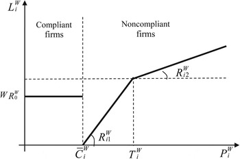
The levy schedules differ between water pollution and air pollution and across different regimes. In the pre-2003 regime, as shown in the left part of figure 1, the levy on wastewater discharge for a compliant firm is based on the total volume of wastewater discharge (W) and the levy rate (R 0 W ):
 $$L_i^w = W R_0^W.$$
A uniform levy rate of 0.05 Chinese Yen (CNY) per ton of wastewater discharge was used in the pre-2003 regime. Figure 1 also illustrates the block levy rates paid by non-compliant firms in the pre-2003 regime. Formally, the potential levy on pollutant i for a non-compliant firm is:
An illustration of the levy system for wastewater in the pre-2003 regime

 $$L_i^w = \left\{\matrix{R_{i1}^W p_i^W \hfill &\hbox{if } p_i^W \le T_i^W\cr R_{i1}^W T_i^W + R_{i2}^W \lpar p_i^W - T_i^W\rpar \hfill &\hbox{if } p_i^W \gt T_i^W} \right.$$
where T
i
W
is the regulatory threshold separating the discharge higher than the standards from the within-standard discharge; R
i1
W
and R
i2
W
are the levy rates for the within discharge and discharge that exceed the standards where R
i1
W
> R
i2
W
; and p
i
W
is a discharge factor that depends on both the total wastewater discharge volume and the degree to which pollutant concentration exceeds the discharge standard, i.e.,
 $p_{i}^{W} = \max \lcub 0\comma \; W\lpar C_{i}^{W} - {\bar C}_{i}^{W}\rpar /{\bar C}_{i}^{W}\rcub $
. The discharge factor varies by pollutants and industry sectors. The central government determines the regulatory threshold and levy rates for each pollutant, T
i
W
, R
i1
W
and R
i2
W
. All three parameters are invariant within each industry sector and across geographic regions.
The concentration standards vary by pollutants and industry sectors (see table A1 in the online appendix, available at http://journals.cambridge.org/EDE for more details). The pulp paper sector, for example, is subject to looser standards for three main water pollutants, namely, COD, BOD (biochemical oxygen demand) and TSS (total suspended solids), than the textile and beverage sectors. BOD has a lower concentration standard than COD and TSS. The levy rates for COD, SO2 and TSS are shown to be decreasing block rates – CNY 0.18 per ton for within-standard discharge and CNY 0.05 for the discharge higher than the standards for both COD and BOD; the corresponding numbers are CNY 0.03 and CNY 0.01 for TSS. The amount of levy for water pollution that a non-compliant firm has to pay is the largest levy among all water pollutants:
 $$L^w = \max \lcub L_1^w\comma \; L_2^w\comma \; \cdots \comma \; L_n^W\rcub$$
where n is the total number of relevant water pollutants discharged by the firm.
In the case of air pollution, only non-compliant firms are subject to pollution levies. For air pollutant i, we denote the levy rate by R
i
a
, the pollutant concentration by C
i
a
, and the corresponding concentration standard by
 ${\bar C}_{i}^{a}$
. The potential levy of air pollutant i for a non-compliant firm is
 $$L_i^a = \max \lcub 0\comma \; R_i^a V\lpar C_i^a - {\bar C}_i^a\rpar \rcub$$
where V is the total discharge of air pollutant i measured in cubic meters. Unlike the water pollution levy for non-compliant firms (see equation (2)), the air pollution levy is assessed on the absolute, rather than percentage, deviation from the concentration standard. Table A1 provides values of the key parameters for two common air pollutants, SO2 and TSP (total suspended particles). A special regulation is imposed on SO2 discharge among non-compliant firms in the acid rain and/or SO2 control areas (including most coastal areas); however, a uniform levy rate, CNY 0.2 per kg of SO2 emission, is applicable regardless of the concentration level.
The pre-2003 levy system has been greatly criticized. It lacks incentives or even provides disincentives to pollution control and abatement because of the decreasing block levy rates for water pollutants, the air pollution levy being not applicable to compliant firms, and constant rates that are not adjusted for inflation (the real value of the later years was substantially lower than in the early years). The levy system was significantly amended in 2003 and called for two steps to calculate the levy amount in the post-2003 regime. The first step is to convert discharge into either COD equivalent for water pollutants or SO2 equivalent for air pollutants:
 $$E_i^K = \left\{\matrix{W C_i^W/e_i^W \hfill &\hbox{for water pollutants} \hfill \cr V C_i^A/e_i^A \hfill &\hbox{for air pollutants} \hfill} \right.$$
where the regulatory conversion parameters for pollutant i are denoted by e i W for water pollution and e i A for air pollution. The conversion parameter takes a value of 1 for COD and 0.95 for SO2. Equation (5) suggests that both compliant and non-compliant firms need to pay for pollution discharge. The pollutants that are more likely to cause environmental damages are assigned with a smaller conversion parameter and have a greater amount of the equivalents. The equivalent is calculated for all pollutants in each pollution type k, but only the top three pollutants with the greatest equivalent matter in calculating the levy amount:
 $$L_k = R_k \sum_{i = 1\comma 2\comma 3} E_i^K$$
where the levy rate R equals CNY 0.7 per unit of COD equivalent and CNY 0.6 per unit of SO2 equivalent for the within-standard discharge, but the rates are doubled for the discharge higher than the standards, i.e., CNY 1.4 and CNY 1.2 for COD and SO2 equivalent, respectively. In the case of air pollution, all polluting firms, whether they are a compliant or non-compliant firm, need to pay the levy. The rates are the same for firms located in the acid rain and SO2 control area or other areas.
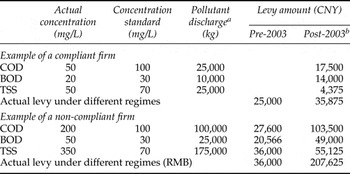
To illustrate the differences between the pre- and post-2003 levy systems, we assume there are two firms, one compliant firm and one non-compliant firm. As shown in table 1, each emits a total of 500,000 tons of wastewater with three particular pollutants, COD, BOD and TSS. The levy for the compliant firm under the post-2003 levy regime totals up to CNY 35,875, increasing from the pre-2003 level of CNY 25,000 by 43.5 per cent. For the non-compliant firm, the levy under the post-2003 regime is almost six times the levy under the pre-2003 regime, changing from CNY 36,000 to CNY 207,625. The numerical comparisons show that the post-2003 levy system penalized all polluters more than the pre-2003 system did and penalized heavy polluters substantially more.
Numerical comparison of potential levy under different regimes (pre- and post-2003)

a We assume the total amount of wastewater discharge is 500,000 tons in both examples. The pollutant discharge is the total wastewater discharge multiplied by the concentration of the corresponding pollutant. b The conversion parameters for COD, BOD and TSS are one, half and four, respectively.
2.2. Pollution quantity control
China first adopted pollution quantity control to regulate pollution in the environmental special zonesFootnote 3 during the 9th and 10th Five-Year Plan periods. The national pollution quantity control imposed on COD and SO2 was elaborated in the 11th Five-Year Plan period (2005–2010), released in 2006. The goal was to reduce major pollutant discharges by 10 per cent relative to the 2005 levels by the end of the 11th Five-Year Plan period (2006–2010). In other words, the target was to reduce China's national emissions from 14.14 million tons in 2005 to 12.73 million tons in 2010 for COD and from 25.49 to 22.94 million tons for SO2. The national pollution control target was further decomposed into the provincial and local levels. The greatest reductions required for COD were in Hebei, Jiangsu and Zhejian provinces – more than 15 per cent of their levels in 2005. Similarly, the great reductions required for SO2 were in Beijing, Shanghai and Shandong – more than 20 per cent of their levels in 2005. Hainan, Qinghai, Xinjiang and Xizang (Tibet) provinces were not required to reduce their COD and SO2 emissions, but were required to maintain their 2005 levels (see figure A1 in the online appendix for more details). The provincial control targets were then decomposed into the city/county level and finally to individual firms. For instance, a COD quota given to a firm was calculated by its total production in the base year of 2005 multiplied by the standard of wastewater discharged for each unit of production and then multiplied by the corresponding concentration standard of COD, where the standard of wastewater discharged per unit of production was designed to incorporate the local COD control target.
In order to achieve the quantity control targets for COD and SO2 by the end of 2010, China implemented a number of policies. For example, whether the region had achieved the local target of pollution control became an important criterion to evaluate local officials' performance and promotion. SEPA was elevated to become the Ministry of Environmental Protection (MEP) in March 2008, which strengthened its position in ensuring compliance with environmental regulations. The minister of MEP claimed that ‘T[t]he total amount control targets have been successfully achieved and the environmental quality of China has been significantly improved over the past 5 years [2005–2010]’ as ‘during the 11th Five-Year Plan Period, China has conducted total amount control of major pollutants. Relative to the 2005 level, COD discharge went down by 12.45 per cent and SO2 by 14.29 per cent, which exceeded the target level of 10 per cent’. However, rigorous research was not found to have examined the role of the pollution quantity control.
2.3. Other pollution control instruments
China has implemented different types of pollution control instruments including command-and-control, market incentives instruments, voluntary instruments and information disclosure (see details in online appendix table A2). Below we discuss specific instruments implemented or enforced in recent years.
Like other developing countries, China lacks the technical and administrative capacity for the effective monitoring and enforcement of environmental laws, regulations and standards to employ command-and-control instruments effectively. China has adopted pollution control instruments that provide economic incentives to firms. For example, emission permit trading of COD was first introduced in 2008 in the Tai Lake area, an environmental specific zone (Bi and Liu, Reference Bi, Liu, Bi, Otsuka, Ge and Wang2009).Footnote 4 Similar permit trading systems have been adopted in other geographical areas and applied to other pollutants. For instance, Chongqing, Shaanxi and Liaoning provinces established their own COD permit trading market in 2010; Chongqing and Shaanxi provinces started trading SO2 emission permits in 2009 and 2010, respectively.
However, market failures and weak institutional support may limit the effectiveness of market-based instruments. China also used voluntary instruments to induce voluntary pollution control, such as state environmental friendly firm labeling, ecological friendly labeling and the voluntary reduction of greenhouse gas emissions program.Footnote 5 On the other hand, corporate performance rating and disclosure (PRD) reduces the information asymmetry between polluters and environmental stakeholders (e.g., consumers, communities, NGOs, investors), empowering these stakeholders to pressure polluters for improved environmental performance (Kennedy et al., Reference Kennedy, Laplante and Maxwell1994; Foulon et al., Reference Foulon, Lanoie and Laplante2002; Bui and Mayer, Reference Bui and Mayer2003; Oberholzer-Gee and Mitsunari, Reference Oberholzer-Gee and Mitsunari2006). The literature has documented the positive effects of PRD programs on regulatory compliance (Wang et al., Reference Wang, Bi, Wheeler, Wang, Cao, Lu and Wang2004; Dasgupta et al., Reference Dasgupta, Wang, Wheeler, Tietenberg and Folmer2007; García et al., Reference García, Sterner and Afsah2007, Reference García, Afsah and Sterner2009). In 1999 China launched its first pilot program of PRD called the Green Watch program in Zhenjiang City, Jiangsu province and Hohhot City, Inner Mongolia Autonomous District. The Green Watch Program rates firms' environmental performance from best to worst by five colors and discloses firms' color ratings to the public. It improved the compliance rates and decreased pollution discharge and pollution intensity (Wang et al., Reference Wang, Bi, Wheeler, Wang, Cao, Lu and Wang2004; Jin et al., Reference Jin, Wang and Wheeler2010). Given the success of its pilot program, the Green Watch program was extended to Jiangsu province in 2001, to eight other provinces during 2003–2005, and promoted to a nationwide implementation since 2005. The Chinese government adopted two critical disclosure measures to improve environmental transparency effectively on 1 May 2005, namely, Government Information Disclosure Regulations (hereafter Regulations) by China's State Council and provisional Environmental Information Disclosure Measures (hereafter Measures) by the MEP. The Regulations state that citizens, legal persona and other organizations have the right to obtain government information by lawful means. The Measures stipulate that: (1) firms listed for violating discharge standards or exceeding discharge quota limits are required to publish their discharge data within 30 days in local media and register the data with the local government agency; (2) non-compliant polluting firms are required to publish their discharge data by relevant local government agencies; (3) the environmental agencies will be legally bound to disclose the list of polluters within 20 days through different channels. If the government agencies fail to fulfill the requirements, the public is entitled to apply for the disclosure and the environmental agencies are required to respond within 15 days. If the agencies turn down the public application for disclosure, the public may report this to the superior environmental authority and/or apply for administrative review or file administrative suits.
To promote corporate social responsibility (CSR) and to foster environmentally and socially sustainable private sector development, the stock markets in China took initiatives. The Shenzen Stock Exchange and the Shanghai Stock Exchange issued voluntary CSR guidance for their listed companies in early 2006 and May 2008, respectively. The MEP and the China Securities Regulatory Commission (CSRC) jointly launched the ‘Green Securities’ policy in February 2008 and then the ‘Green IPO’ policy in June 2008. The Green Securities policy aims to make it harder for polluting firms to raise capital by requiring publically traded companies to disclose information about their environmental record. The Green IPO policy requires firms who want to apply for an initial IPO to include their environmental performance assessment evaluated by the MEP along with financial records for the 36 months in their application before initiating an IPO or receiving refinancing from banks. The MEP conducts assessments and calls for public opinions during a 10-day pre-IPO evaluation period. The applicant firm cannot further pursue an IPO without approval from the MEP. Between February 2008 when the policy was first implemented and September 2008, 20 out of 38 companies were rejected for further review of IPOs because of this procedure (Siddy, Reference Siddy2009). The CSRC and the MEP developed a guide on environmental information disclosure of publically listed companies in September 2010, which requires the listed companies to disclose their environmental performance regularly and to report environmental accidents within 24 hours of their occurrence.
We are not able to estimate the effectiveness of these most recently implemented policies because of the lack of available data. Our empirical analyses mainly focus on the pollution levy system and pollution quantity control.
3. A brief literature review of pollution control in China
A rich literature investigates environmental regulations and industrial pollution control in China with a focus on the effectiveness of the levy system. The literature has documented a negative association between the levy rates and pollution discharge and/or pollution intensity based on either firm-level pollution data (Dasgupta et al., Reference Dasgupta, Laplante, Mamingi and Wang2001; Wang et al., Reference Wang, Mamingi, Laplante and Dasgupta2003; Wang and Wheeler, Reference Wang and Wheeler2005; Wang and Jin, Reference Wang and Jin2007) or provincial data (Jiang and McKibbin, Reference Jiang and McKibbin2002). Jiang and McKibbin (Reference Jiang and McKibbin2002) find that the pollution levy effectively reduces water pollution, air pollution and solid wastes discharge. The actual levy that a polluting firm pays (hereafter the effective levy) may deviate from what it deserves to pay. Consequently, the effective levy rate, which is the actual levy payments divided by the total pollution discharge, may deviate from the official levy rate. The significant disparity in the effective levy rates may be due to differences in ownership structures, economic development and strictness of environmental enforcement (Jiang and McKibbin, Reference Jiang and McKibbin2002; Wang and Wheeler, Reference Wang and Wheeler2005). Wang and Wheeler (Reference Wang and Wheeler2005) state two possible channels through which provincial and local environmental authorities can affect the size of the effective levy. First, concentration standards, a critical factor in calculating the levy amount, are jointly set by local and central regulators, which can vary by regions. Second, ‘the levy can be reduced or even eliminated at the discretion of local regulators after appropriate inspections’ (Wang and Wheeler, Reference Wang and Wheeler2005: 181). Wang et al. (Reference Wang, Mamingi, Laplante and Dasgupta2003) find that state-owned firms have greater bargaining power with local environmental authorities and, thus, successfully negotiate for a lower effective levy rate, which partly explains these firms' worse environmental performance compared with other firms. Wang and Wheeler (Reference Wang and Wheeler2005) show that relatively affluent, heavily industrialized coastal provinces had the highest effective levy rates for wastewater, while less developed inland provinces had the minimum rates in the pre-2003 regime. The region-variant levy rates play an important role when foreign-directed investment firms choose their location (Di, Reference Di2007; Dean et al., Reference Dean, Lovely and Wang2009).
Different from the ex post self-report in Western countries, firms in China self-report their pollution discharge ex ante (Wang and Wheeler, Reference Wang and Wheeler2005). At the beginning of each year, firms have to register with the local environmental authorities by providing the predicted volume of emissions in the coming year. Environmental authorities verify the registration reports and issue pollution discharge licenses to firms. During the year, firms are required to modify their reports as needed – when their actual emissions are different from those predicted at the beginning of the year. Moreover, environmental authorities conduct field inspections. At the end of each quarter, based on firms' reports and inspections, authorities notify firms about the amount of levies they should pay in this quarter. In case of false reporting (either at the time of the original report or at the time when plants must modify their estimates) and being caught by the authorities, firms are liable to pay the evaded levy and between 100 per cent and 300 per cent extra for penalties. When a plant badly underreports and is caught, besides the regular penalty it also faces a fixed amount of additional penalty. The total monetary penalty should not exceed the ceiling of CNY 100,000 (around US$16,000). Other non-monetary penalty instruments are also available, such as revoking discharge licenses and shutting down facilities, but they are rarely used. The ex ante self-report and limited penalties for a false report lead to weak enforcement (Wang and Wheeler, Reference Wang and Wheeler2003; Lin, Reference Lin2011). For instance, firms can strategically underreport their pollution at the beginning of the year and decide whether to modify their report by observing if they are inspected or not. To induce a truthful self-report, both expected and unexpected site inspections are occasionally conducted by local environmental authorities. Dasgupta et al. (Reference Dasgupta, Laplante, Mamingi and Wang2001) show that the frequency of such inspections is negatively associated with firms' pollution levy. Lin (Reference Lin2011) provides a theoretical framework to support the effect of inspections in inducing truthful reporting among polluting firms, and the empirical results confirm the expectations.
4. The model
The empirical analysis consists of two parts. We first estimate technical efficiency using DEA and then investigate factors affecting technical efficiency and pollution intensity. We employ an R-package for DEA and Stata for regression analyses.
4.1. Estimation of technical efficiency
Technology and environmental management is an important determinant of pollution (Managi and Kaneko, Reference Managi and Kaneko2009). Using time trend variables to proxy technology changes (a common practice in the existing literature) is likely to capture any time-varying effects that are not necessarily related to technology. Thus, it is important to explicitly estimate technical efficiency. There is an ongoing debate whether deterministic methodologies such as DEA or stochastic methodologies such as stochastic frontier analysis should be used (Bravo-Ureta et al., Reference Bravo-Ureta, Solis, Moreira López, Maripani, Thiam and Rivas2007). Using a meta-analysis to review empirical studies investigating agricultural technical efficiency in developing countries, Thiam et al. (Reference Thiam, Bravo-Ureta and Rivas2001) find no statistically significant differences in these estimates between using stochastic and deterministic approaches. Managi and Kaneko (Reference Managi and Kaneko2009) employ DEA to explicitly estimate technical efficiency and then incorporate it as one of the determinants of pollution abatement. We use a similar approach, but our focus is on the effectiveness of technical efficiency on pollution control.
DEA, developed by Charnes (Reference Charnes1978), is a non-parametric methodology for evaluating the relative efficiency of a set of comparable entities called decision making units (DMUs) with multiple inputs and outputs. It has gained popularity in environmental performance measurement by incorporating undesired output (pollution) along with the desirable output (production) in the traditional DEA framework (Zaim, Reference Zaim2004; Zhou et al., Reference Zhou, Poh and Ang2007, Reference Zhou, Ang and Poh2008a, Reference Zhou, Ang and Pohb; Li, Reference Li2010) for a detailed review of DEA in energy and environmental studies.
Suppose we observe a sample of I DMUs. Each of them use N different inputs X = (x 1,x 2,…,x N ) ∈ R + N to produce M different desirable outputs Y = (y 1,y 2, …,y M ) ∈ R + M , and K different undesirable outputs (pollution) Z = (z 1, z 2, …,z K ) ∈ R + K . The production technology can be characterized by T = {(X,Y,Z):X produce (Y, Z)}. Besides satisfying standard regularity conditions like convexity and closeness (see details at Fare and Primont, Reference Fare and Primont1995; Cooper et al., Reference Cooper, Seiford and Tone2006), the technology T(X, Y, Z) also satisfies the following two properties to account for negative production externalities:
P1
Outputs are weakly disposable, i.e., if (X, Y, Z) ∈ T and 0 ≤ θ≤ 1, then (X,θY,θZ) ∈ T.
P2
Desirable and undesirable outputs are null-joint, i.e., if (X, Y, Z) ∈ T and Z = 0, then Y = 0.
P1 suggests that the proportional reduction in desirable and undesirable outputs is feasible. For example, to reduce pollution (undesirable output), a proportionate reduction in desirable output is needed. P2 implies that production with only desirable outputs is impossible, and the only way to eliminate all undesirable outputs is to stop production.
Technical efficiency is the ability of a decision maker to maximize output with given quantities of inputs and certain technology (output-oriented), or the ability to minimize input uses with a given output target (input-oriented). Output-oriented technical efficiency is commonly used. In particular, following Tyteca (Reference Tyteca1997) the technology efficiency for DMU i at time t is defined as
 $$TE^{it} \lpar X^{it}\comma \; Y^{it}\comma \; Z^{it}\rpar =\max \lcub \phi \colon \lpar X^{it}\comma \; Y^{it}\comma \; Z^{it} /\phi\rpar \in T^{it}\rcub .$$
We define two types of outputs: the undesired environmental output that is denoted by Z and measured by COD- and SO2-equivalent emissions, and the desired output that is denoted by Y and measured by provincial gross industry productivity. The production inputs denoted by X consist of labor and capital. Equation (7) suggests that an improvement in technology efficiency shifts the production possibility frontier (PPF) outwards since more can be produced from the same amount of inputs given the improvement. Following equation (7), the technical efficiency score (TES) of province i at time t is
 $${TES}^{i\comma t} = {TE^{i\comma t} \lpar X^{i\comma t}\comma \; Y^{i\comma t}\comma \; Z^{i\comma t}\rpar \over \max\limits_{i\comma t} TE^{i\comma t} \lpar X^{i\comma t}\comma \; Y^{i\comma t}\comma \; Z^{i\comma t}\rpar }$$
A greater TES implies higher technical efficiency.
We then investigate provincial variations of technical efficiency by employing econometric models. We assume that technical efficiency in province i at time t denoted by TE it is a function of input prices (PXit) consisting of labor wage and capital cost, pollution control variables (levy rates and quantity control targets) represented by Q it , province-specific economic factors (M it ), region-specific time trends (γ i ), and province effects (θ i ). The reduced structural equation for technical efficiency is
 $$TE_{it} = \theta_i + \gamma_i t + \beta_1 PX_{it} + \beta_2 Q_{it} + \beta_3 M_{it} + \varepsilon_{it}.$$
We expect β1 to be positive because a higher input price is expected to provide an incentive for being more technically efficient. We also expect β2 to be positive because a higher levy rate or a larger quantity control target also gives firms an incentive to improve technical efficiency so that the undesirable output (pollution) can be reduced. The province-specific economic factors include the percentage of the population aged 15 and above who have at least tertiary education, GDP per capita, and ownership structures (measured by share of GDP contributed by state-owned enterprises, collectively owned enterprises, foreign investment and private companies). We expect that technical efficiency relates to investment in research and technology (Nishimizu and Page, Reference Nishimizu and Page1982; Ahmad and Bravo-Ureta, Reference Ahmad and Bravo-Ureta1996), but such data is not available from the 1990s. We use the annual count of patent applications as a proxy for investment in research and technology.
4.2. Investigating the role of the pollution control system and technical efficiency
We use the following reduced form to investigate the effectiveness of technical efficiency, pollution control instruments and prices of production inputs on pollution intensity:
 $$S_{ijt} = \vartheta_i + \rho_i t + \varphi TE_{it} + \alpha_1 M_{it} + \alpha_2 PX_{it} + \propto_3 Q_{it} + \mu_{it}$$
where S ijt is the intensity of either COD or SO2 equivalent discharge (index by j) in province i at time t and TE it is the estimated technical efficiency. Equation (10) is consistent with the three emission determinants proposed by Grossman (Reference Grossman, Goldin and Winters1995) and Grossman and Krueger (Reference Grossman and Krueger1991): (a) the scale effect that measures change in economic activity represented by the provincial economic variables such as gross output; (b) the composition effect that measures the structural economic changes, substitutions between inputs and the tradeoff between inputs and undesirable output; (c) the technique effect that measures changes in energy/resource intensity, represented by technical efficiency. Equation (10) estimates the effect of key variables of interest on pollution intensity, including φ for technical efficiency; α's for effective levy rates of water and air pollution, the pollution quantity control targets, and pollution abatement costs.
5. The data
We rely on various China Statistics Yearbooks for province-level economic data and China Environmental Yearbooks for pollution-related variables to compile a panel data set for 26 provinces and four provincial level municipalities (Beijing, Tianjin, Shanghai and Chongqing) in 1992–2008. The panel data for provincial output values, wage and effective levy rates are adjusted by the provincial producer price index (PPI) and the capital input price is adjusted by the provincial price index of capital investment (PPC) in fixed assets. Both the PPI and PPC are released by China's National Bureau of Statistics.
Overall, the provincial average GDP per capita is approximately CNY 2,300. The state-owned enterprises contributed more than half of the industry output, followed by privately owned companies (15 per cent), collectively owned (10 per cent) and foreign invested companies (7 per cent). Approximately 20 per cent achieve at least tertiary education. See online appendix table A3 for the summary statistics of the economic and pollution variables.
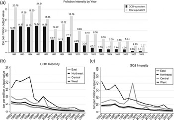
We measure pollution intensity by the COD equivalent of water pollutants and the SO2 equivalent of air pollutants per million gross industrial output values. On average, for each million output value, approximately 4 tons of COD equivalent, and 10 tons of SO2 equivalent was discharged (see table A3). As shown in figure 2(a), the data clearly show a declining trend of pollution intensity. The COD intensity decreased by more than 80 per cent from 10.46 to 1.55 ton per million output value from 1992 to 2003; it also decreased by more than 67 per cent from 2003 to 0.51 in 2008. Similarly, the SO2 intensity was almost halved, decreasing from 20.78 in 1992 to 6.16 in 2003, and more than halved from 2003 to 2.27 in 2008.
Pollution intensity by year and economic region

Traditionally, China is divided into four economic regions mainly based on geographical locations and economic development levels: East, Northeast, Central and West.Footnote 6 The East region is most economically developed, while the West region is the least developed. As shown in figures 2(a) and 2(b), we find a decreasing trend of pollution intensity in each economic region and significant variations of pollution intensity between economic regions, especially in the pre-2003 regime. In general, the pollution intensity was highest in the West region, followed by the Central region, and lowest in the East and Northeast regions. Take 2008 as an example: compared with the East region, where the average pollution intensity of COD was 0.15 tons per million real value of industrial output, the COD intensity more than doubled in the Northeast region (0.38), more than tripled in the Central region (0.53), and quadrupled in the West region (0.85). Similarly, the 2008 SO2 intensity was lowest in the East region (0.72) followed by Northeast (1.47), Central (2.46) and West (3.92).
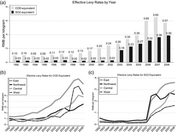
The literature has documented a significant regional disparity of the effective levy rates in the 1990s (Jiang and McKibbin, Reference Jiang and McKibbin2002; Wang and Wheeler, Reference Wang and Wheeler2003, Reference Wang and Wheeler2005). As shown in figures 3(b) and 3(c), we find a similar trend in the case of water pollutants in the pre-2003 regime – the effective levy rates were highest in the East region and lowest in the West region, but the difference in the effective levy rates for air pollutants was less pronounced between regions in this regime. The post-2003 data demonstrate even wider regional disparities in the effective levy rates for both water and air pollution. For example, the levy rate in 2008 varied from CNY 0.07 per ton of COD equivalent in Guangxi to CNY 2.54 in Tibet, and from CNY 0.11 per ton of SO2 equivalent in Guangxi to CNY 1.13 in Shanxi. However, the significant disparity in the effective levy rates does not necessarily imply that the system was ineffective. The disparity may be responsive to ambient quality and economic development, thus reflecting the cost efficiency of pollution abatement (Jiang and McKibbin, Reference Jiang and McKibbin2002; Wang and Wheeler, Reference Wang and Wheeler2005).
Effective levy rates by year and economic region

6. Results and discussion
6.1. Estimated technical efficiency
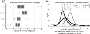
Figures 4(a) and 4(b) show significant regional differences of technical efficiency. On average, technical efficiency was much higher in the Northeast region (0.51), followed by the East region (0.44), the Central region (0.36), and lowest in the West region (0.31). Figure 4(a) shows that the East region was characterized by a few highly technically efficient provinces, while the West region had provinces with high and low technical efficiency.
Estimated technical efficiency

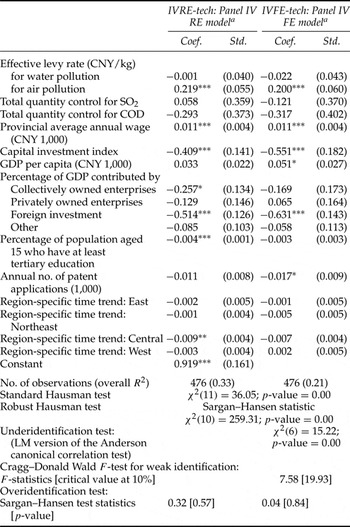
Following equation (9) we explore the factors that affect technical efficiency and present the results of both fixed effect (FE) and random effects (RE) models in Table 2. Both RE and FE models are estimated with robust standard errors clustered on province to account for correlation within provinces. The standard Hausman test rejects the null hypothesis that an RE model provides consistent estimates as the test statistic overall equals 36.02, which exceeds the critical value at the 1 per cent significance level (p-value = 0.000) (see table 2). However, a serious shortcoming of the standard Hausman test is that it requires the RE estimator to be efficient. Wooldridge (Reference Wooldridge2002) proposes performing the Wald test using cluster-robust standard errors. The robust Hausman test also rejects the null hypothesis and favors the FE model – the Sargan–Hansen statistic (259.31) exceeds the critical value at the 1 per cent significance level (p-value = 0.000) (see Table 2). We therefore conclude that the FE model fits the data better and mainly discuss the estimation results of the FE model.
Panel estimation results of technical efficiency

Notes: ***, ** and * represent 1%, 5% and 10% of statistical significance, respectively.
a The excluded instruments for provincial GDP per capita are national GDP per capita and opened to trade measured by the ratio of total imports and exports to the gross GDP.
GDP per capita is likely to be endogenous. For example, the possible omitted variable for research and development investment may affect GDP per capita. We use a panel IV fixed effects model to control for potential endogeneity of GDP per capita, where the instruments we propose are national GDP per capita and openness to trade measured by the ratio of total imports and exports to gross GDP. Several statistical tests are performed to validate the instruments (see Table 2). First, the LM version of the Anderson canonical correlation test (Anderson, Reference Anderson1951) rejects the null hypothesis of under-identification, which suggests that two instrument variables are correlated with GDP per capita. Second, the Sargan–Hansen test is conducted to test for over-identifying restrictions. The result provides strong evidence that we cannot reject the null hypothesis that the instruments are valid instruments, i.e., uncorrelated with the error term, and that the excluded instruments are correctly excluded from the estimated equation. The test results for under-identification and over-identification suggest the proposed instrument variables meet the relevance and exogeneity conditions. However, the Cragg–Donald Wald statistic (7.58) is smaller than the critical value at the 10 per cent significance level (19.93) and, thus, we fail to reject the null hypothesis of weak instruments.
The results suggest that wage has a positive effect, but capital cost has a negative effect on technical efficiency, while both effects are statistically significant at the 1 per cent level. The above findings suggest that an increase of wage or a decrease in capital cost is associated with an improvement in technical efficiency. The results may partially explain that the West region is found to be lower in technical efficiency, but more labor and pollution intensive than the East region. The total number of employees per unit of gross output value and pollution intensity of SO2 equivalent in the West region was more than triple that in the East region, but technical efficiency was lower by 28 per cent on average. We find no statistically significant effect of the quantity control targets on technical efficiency. The effective levy rate for air pollution has a statistically significant effect on technical efficiency – the higher the effective levy rate, the higher the technical efficiency. However, the effective rate of water pollution is not statistically significant.
Table 2 also shows that GDP per capita has a positive, statistically significant effect on technical efficiency, which suggests that the more economically advanced provinces tend to have higher technical efficiency. We find that the percentage of GPD contributed by different ownership structures has no statistical difference in technical efficiency with only one exception for foreign investment. Technical efficiency is lower if a greater share of GDP is contributed by foreign investment compared with that by state-owned enterprises. Another surprising result is that the annual number of patent applications is statistically and negatively associated with technical efficiency at the 10 per cent level.
6.2. Estimation results on intensity of COD- and SO2-equivalent
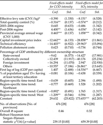
Based on the specification in equation (10), we conduct panel estimations of pollution intensity for COD and SO2 equivalent. As reported in table 3, the robust Hausman test favors an FE model for both COD and SO2 intensity as the Sargan–Hansen test statistics exceed the critical value at the 1 per cent significance level (χ2(16) = 239.15 for COD and χ2(16) = 659.39 for SO2). Second, in both estimations we use the first lag of GDP per capita in logarithm to avoid endogeneity.
Estimation results of pollution intensity of COD- and SO2-equivalent

Notes: ***, ** and * represent 1%, 5% and 10% of statistical significance, respectively. Numbers in parentheses are standard deviations. a The levy and total amount control are specific for COD- or SO2-equivalent. Similarly, pollution abatement costs refer to water pollution abatement costs for COD intensity, and air pollution abatement for SO2 intensity.
We can draw the following conclusion based on the estimation results presented in table 3. First, pollution control instruments are found to be effective in reducing pollution intensity. Both the effective levy rate and the pollution quantity control targets have a negative, statistically significant effect on pollution intensity except for the effective levy rate for the COD intensity (negative but insignificant). Other than these two main pollution control instruments, the regime change does not lead to statistically significant differences in pollution intensity in the 2003–2006 regime compared with the pre-2003 regime for both COD and SO2 intensity, but the post-2006 regime is characterized by a higher pollution intensity for both COD and SO2 compared with the pre-2003 regime. Second, technical efficiency has a negative, statistically significant effect on pollution intensity for both COD and SO2. Third, input prices play important roles. The higher the labor cost and/or the lower the capital cost, the higher the pollution intensity. However, pollution abatement cost does not have a statistically significant effect on pollution intensity. Table 3 also suggests that a high income level is associated with lower pollution intensity, as shown by the coefficient of the first lag of GDP per capita in logarithm.
7. Conclusions and policy implications
Using the provincial economic and pollution data in China, we first estimate technical efficiency using the DEA approach and then investigate the role of technical efficiency, prices of production inputs, and policy instruments, namely, pollution levy and pollution quantity control, on pollution intensity. The results suggest significant regional differences in technical efficiency, effective levy rates and provincial targets of total pollution quantity control. We also show that prices of production inputs play important roles in both technical efficiency and pollution intensity. Technical efficiency is higher if there is an increase in the effective pollution levy rate (of air pollution) or labor wage, or a decrease in capital cost. On the other hand, technical efficiency, the effective levy rates, pollution quantity control targets and capital cost have a negative effect but wage has a positive effect on pollution intensity of both COD and SO2.
This study offers the following contribution to the literature. First, to our knowledge it is the first study to explicitly investigate technical efficiency in pollution intensity in the context of China, as previous studies have used time trends to control for technical efficiency and changes. Second, the majority of previous studies utilize the data in the pre-2003 regime and focus on one policy instrument, the levy system. With the expansion of the data, we are able to convert pollution discharge into COD and SO2 equivalents and investigate the effectiveness of two main pollution control instruments, the levy system and total quantity control. From this standpoint, this study provides a more complete analysis and it is able to offer broader policy implications.
This study provides the following policy implications. First, pollution quantity control effectively reduces pollution intensity but it does not improve technical efficiency. We speculate that one of the main approaches to meet the quantity control target is to shut down large polluters, which leads to reduced pollution intensity but no change in technical efficiency. On the other hand, the effective levy rates for air pollution are associated with improvement in both pollution intensity and technical efficiency. Pollution levy, a market-based instrument, may work better than command-based instruments like pollution quantity control as it gives polluters an incentive to improve technical efficiency that will lead to a long-run improvement in pollution control. Second, the prices of production inputs play important roles in technical efficiency and pollution intensity, which provide alternative channels for China to control industrial pollution. On the other hand, it also cautions the government of the unintended consequence on the environment if any policy changes are made relating to labor and capital costs.