1 Introduction
Free liquid jets offer some of the most fascinating and beautiful phenomena in fluid mechanics. Probably the most familiar of these is the ‘liquid rope-coil’ effect (Barnes & Woodcock Reference Barnes and Woodcock1958) which occurs when a thin stream of honey falls onto a piece of toast. If the fall height is large enough, the falling stream builds a whirling corkscrew-like structure which resembles a pile of coiled rope played out by a mountaineer. Liquid rope coiling has been extensively studied, using laboratory experiments (Barnes & Woodcock Reference Barnes and Woodcock1958; Barnes & MacKenzie Reference Barnes and MacKenzie1959; Cruickshank Reference Cruickshank1980; Cruickshank & Munson Reference Cruickshank and Munson1981; Huppert Reference Huppert1986; Griffiths & Turner Reference Griffiths and Turner1988; Mahadevan, Ryu & Samuel Reference Mahadevan, Ryu and Samuel1998; Maleki et al. Reference Maleki, Habibi, Golestanian, Ribe and Bonn2004; Habibi et al. Reference Habibi, Maleki, Golestanian, Ribe and Bonn2006, Reference Habibi, Rahmani, Bonn and Ribe2010, Reference Habibi, Hosseini, Khatami and Ribe2014; Ribe et al. Reference Ribe, Huppert, Hallworth, Habibi and Bonn2006b ; Ribe, Habibi & Bonn Reference Ribe, Habibi and Bonn2006a ), linear stability analysis (Cruickshank Reference Cruickshank1988; Tchavdarov, Yarin & Radev Reference Tchavdarov, Yarin and Radev1993; Ribe et al. Reference Ribe, Habibi and Bonn2006a ), scaling analysis (Mahadevan, Ryu & Samuel Reference Mahadevan, Ryu and Samuel2000), asymptotic analysis (Blount Reference Blount2010) and numerical analysis based on slender-rope theory (Maleki et al. Reference Maleki, Habibi, Golestanian, Ribe and Bonn2004; Ribe Reference Ribe2004; Habibi et al. Reference Habibi, Maleki, Golestanian, Ribe and Bonn2006, Reference Habibi, Rahmani, Bonn and Ribe2010, Reference Habibi, Hosseini, Khatami and Ribe2014; Ribe et al. Reference Ribe, Huppert, Hallworth, Habibi and Bonn2006b ,Reference Ribe, Habibi and Bonn a ).
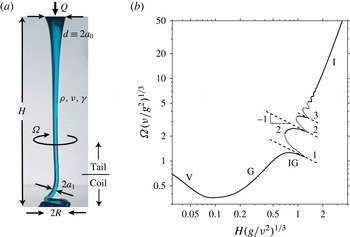
(a) Parameters of a typical laboratory setup used to study liquid rope coiling. Fluid with density
 $\unicode[STIX]{x1D70C}$
, kinematic viscosity
 $\unicode[STIX]{x1D708}$
and coefficient of surface tension
 $\unicode[STIX]{x1D6FE}$
is ejected at a volumetric rate
 $Q$
from a nozzle of diameter
 $d$
and falls a distance
 $H$
onto a rigid surface, where it forms a coil of radius
 $R$
. The radius of the rope in the coil is
 $a_{1}$
, and the angular frequency of coiling is
 $\unicode[STIX]{x1D6FA}$
. (b) Coiling frequency as a function of height, calculated numerically for
 $d(g/\unicode[STIX]{x1D708}Q)^{1/4}=0.272$
and
 $Q(g/\unicode[STIX]{x1D708}^{5})^{1/3}=3.78\times 10^{-7}$
. The dotted portions of the curve are unstable to small perturbations (Ribe et al.
Reference Ribe, Habibi and Bonn2006a
). The dashed lines show the frequencies of the first three pendulum modes of the tail. The labels V, G, IG and I indicate the portions of the curve corresponding to the viscous, gravitational, inertio-gravitational and inertial modes respectively.

The main result of the aforementioned studies is that liquid rope coiling can occur in four different modes – viscous, gravitational, inertio-gravitational and inertial – depending on how the viscous forces that resist the bending of the rope are balanced. In the viscous (V) mode, both gravity and inertia are negligible, and the coiling is like that of toothpaste squeezed slowly from a tube onto a nearby surface. In the gravitational (G) mode, the viscous forces that resist bending are balanced by gravity. In the inertio-gravitational (IG) mode, the long ‘tail’ of the rope behaves like a distributed pendulum, entering into resonance with the coil when the frequency fixed by the latter is close to one of the natural frequencies of the tail. Finally, in the inertial (I) mode, the viscous forces are balanced by inertia in the coil.
In the laboratory, the principal control parameter that determines which mode obtains is the fall height
 $H$
, which is typically varied while the fluid properties and the flow rate are held constant. Figure 1(a) shows the principal geometric and physical parameters of a typical laboratory set-up. Figure 1(b) displays a numerically calculated curve of coiling frequency versus height, which shows that the coiling modes appear in the order V–G–IG–I as the fall height increases.
The previous studies cited above have given us a remarkably detailed understanding of each of these four modes. However, what is still lacking is a complete regime diagram of the modes as a function of the parameters that control the coiling frequency: the fall height
 $H$
, the fluid viscosity
 $\unicode[STIX]{x1D708}$
, the volumetric flow rate
 $Q$
and the nozzle diameter
 $d$
. Our situation at present is like that of the proverbial blind men exploring the elephant: we have a deep understanding of each of the beast’s individual parts, and our task now is to synthesize them into a synoptic portrait of the whole.
2 Dimensional analysis
If the minor effect of surface tension is neglected, the coiling frequency
 $\unicode[STIX]{x1D6FA}$
depends on
 $H$
,
 $Q$
,
 $\unicode[STIX]{x1D708}$
,
 $d$
and the gravitational acceleration
 $g$
. Of these six parameters, two have independent dimensions. Buckingham’s
 $\unicode[STIX]{x1D6F1}$
-theorem then states that there are four independent dimensionless groups, which I take to be
 $$\begin{eqnarray}\unicode[STIX]{x1D6F1}_{\unicode[STIX]{x1D6FA}}=\unicode[STIX]{x1D6FA}\left(\frac{\unicode[STIX]{x1D708}}{g^{2}}\right)^{1/3},\quad \unicode[STIX]{x1D6F1}_{H}=H\left(\frac{g}{\unicode[STIX]{x1D708}^{2}}\right)^{1/3},\quad \unicode[STIX]{x1D6F1}_{Q}=Q\left(\frac{g}{\unicode[STIX]{x1D708}^{5}}\right)^{1/3},\quad \unicode[STIX]{x1D6F1}_{d}=d\left(\frac{g}{\unicode[STIX]{x1D708}Q}\right)^{1/4}.\end{eqnarray}$$
The parameter
 $\unicode[STIX]{x1D6F1}_{d}$
is the ratio of the nozzle diameter
 $d$
to the length scale
 $$\begin{eqnarray}\unicode[STIX]{x1D6FF}=\left(\frac{\unicode[STIX]{x1D708}Q}{g}\right)^{1/4},\end{eqnarray}$$
which is of the order of the arcwise extent of the bending boundary layer in gravitational coiling (Ribe et al. Reference Ribe, Huppert, Hallworth, Habibi and Bonn2006b ). The dimensionless frequency obeys a law of the form
 $$\begin{eqnarray}\unicode[STIX]{x1D6F1}_{\unicode[STIX]{x1D6FA}}=\text{fct}\left(\unicode[STIX]{x1D6F1}_{H},\unicode[STIX]{x1D6F1}_{Q},\unicode[STIX]{x1D6F1}_{d}\right).\end{eqnarray}$$
The above relationship can be represented by contour plots of
 $\unicode[STIX]{x1D6F1}_{\unicode[STIX]{x1D6FA}}$
as a function of
 $\unicode[STIX]{x1D6F1}_{H}$
and
 $\unicode[STIX]{x1D6F1}_{Q}$
for several values of
 $\unicode[STIX]{x1D6F1}_{d}$
. The ensemble of these plots will be the basis for the regime diagram that is sought.
3 Onset of coiling
The path to a regime diagram naturally starts with a consideration of the onset of coiling. The traditional way to determine the coiling onset criterion is to perform a linear stability analysis of a steady axisymmetric stagnation flow of a fluid jet falling from a nozzle onto a plate some distance below (Tchavdarov et al. Reference Tchavdarov, Yarin and Radev1993). However, the stagnation flow can only be steady if the plate is permeable, and if it is not then the jet must be infinitely wide at the bottom. This serious drawback of the linear stability approach means that we need to seek an alternative criterion for the onset of coiling.
A simple geometrical criterion arises from the fact that there are two distinct length scales in the coil: the radius
 $R$
of the coil and the radius
 $a_{1}$
of the rope itself. Now, coiling can only occur if
 $R\geqslant a_{1}$
; otherwise, the rope would intersect itself in the centre of the coil. Accordingly, Habibi et al. (Reference Habibi, Hosseini, Khatami and Ribe2014) proposed that
 $a_{1}=R$
is the critical condition for the onset of coiling. Since the numerical continuation method of Ribe (Reference Ribe2004) predicts both
 $R$
and
 $a_{1}$
, it can be used to determine the critical surface as a function of
 $\unicode[STIX]{x1D6F1}_{H}$
,
 $\unicode[STIX]{x1D6F1}_{Q}$
and
 $\unicode[STIX]{x1D6F1}_{d}$
. The procedure is to start with a finite-amplitude coiling solution with
 $a_{1}<R$
, and then to continue it numerically until
 $a_{1}$
just equals
 $R$
.
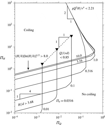
Existence of steady coiling solutions, determined numerically using the method of Ribe (Reference Ribe2004). Each curve is a locus of points where
 $a_{1}=R$
for a given value of
 $\unicode[STIX]{x1D6F1}_{d}=d(g/\unicode[STIX]{x1D708}Q)^{1/4}\equiv d/\unicode[STIX]{x1D6FF}$
. Each curve divides the diagram into regions where steady coiling solutions with
 $a_{1}<R$
exist (above and to the left) and do not exist (below and to the right). Black inverted triangles indicate values of
 $\unicode[STIX]{x1D6F1}_{H}$
above which critical solutions with
 $a_{1}=R$
do not exist. Inequalities give the criteria for the onset of coiling corresponding to different parts of the diagram.

The result of this procedure is shown in figure 2, which displays critical curves
 $a_{1}=R$
for seven different values of
 $\unicode[STIX]{x1D6F1}_{d}\in [0.01,10]$
. These curves are in fact cross-sections of a critical surface in the three-dimensional parameter space
 $(\unicode[STIX]{x1D6F1}_{H},\unicode[STIX]{x1D6F1}_{Q},\unicode[STIX]{x1D6F1}_{d})$
. The logarithms of the values of
 $\unicode[STIX]{x1D6F1}_{d}$
are evenly spaced to assist in identifying intermediate asymptotic limits, of which four are evident. The first is represented by the line with slope
 $-2$
at upper right, where the four curves for
 $\unicode[STIX]{x1D6F1}_{d}\geqslant 0.316$
coincide. Coiling in this limit occurs when
 $gQ^{2}H/\unicode[STIX]{x1D708}^{4}<2.21$
, and corresponds to one variety of the inertial (I) mode, as will be explained below. The second limit occurs for low values of
 $\unicode[STIX]{x1D6F1}_{d}\leqslant 0.1$
for which the upper parts of the critical curves are vertical. Here, coiling occurs when
 $Q/(\unicode[STIX]{x1D708}d)<0.85$
. The inverted triangles in figure 2 indicate where the critical solutions cease to exist, as evidenced by failure of the numerical algorithm. This limit, which corresponds to a second variety of inertial coiling, has not previously been reported to the best of my knowledge. The third and fourth limits are in the left portion of the diagram where inertia is negligible. At lower left, the critical curve with slope
 $1/4$
corresponds to the V mode, for which coiling occurs when
 $H/d>3.68$
. At centre left, the critical curve is that of the G mode, which occurs when
 $(H/\unicode[STIX]{x1D6FF})[\ln (H/\unicode[STIX]{x1D6FF})]^{1/2}>8.0$
. The logarithmic factor in the expressions for the radius
 $R$
and the frequency
 $\unicode[STIX]{x1D6FA}$
of gravitational coiling was first found by Blount (Reference Blount2010).
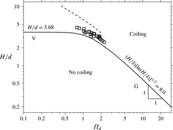
A natural question at this point is whether the critical curves of figure 2 agree with measurements of coiling onset in laboratory experiments. Figure 3 shows the critical curve for the V and G modes, obtained from the leftmost portion of figure 2. The V mode corresponds roughly to
 $\unicode[STIX]{x1D6F1}_{d}<0.5$
, while the G mode obtains for
 $\unicode[STIX]{x1D6F1}_{d}>2$
. Also shown in figure 3 are experimental measurements of the critical fall height for the onset of coiling for small values of the inverse Bond number
 $\unicode[STIX]{x1D6FE}/\unicode[STIX]{x1D70C}gd^{2}$
, where
 $\unicode[STIX]{x1D6FE}$
is the coefficient of surface tension (squares and circles; Cruickshank Reference Cruickshank1980). Finally, the dashed line is the prediction of the critical height for
 $\unicode[STIX]{x1D6FE}=0$
from the linear stability analysis of Tchavdarov et al. (Reference Tchavdarov, Yarin and Radev1993). While the experimental measurements do not agree perfectly with the critical curve
 $a_{1}=R$
, they are significantly closer to that curve than to the prediction of the linear stability analysis. The most likely reason for the remaining discrepancy is that the rope is fairly thick in the parameter range of the experiments, so that the slender-rope approximation upon which the numerical code is based becomes inaccurate. Nevertheless, it seems reasonable to conclude from figure 3 that
 $a_{1}=R$
is an appropriate criterion for the onset of coiling observed in laboratory experiments. In what follows, I shall study numerically how the coiling frequency depends on the dimensionless parameters
 $\unicode[STIX]{x1D6F1}_{H}$
,
 $\unicode[STIX]{x1D6F1}_{Q}$
and
 $\unicode[STIX]{x1D6F1}_{d}$
.
Critical curve
 $a_{1}=R$
(solid line) in the inertia-free (Stokes) limit, separating regions where coiling occurs (above) and does not occur (below). The symbols are experimentally measured critical heights (Cruickshank Reference Cruickshank1980) for silicone oil with
 $\unicode[STIX]{x1D6FE}/\unicode[STIX]{x1D70C}gd^{2}=0.0063$
(circles) and 0.014 (squares), corresponding to the limit of small surface tension. The dashed line is the critical curve predicted by the linear stability analysis of Tchavdarov et al. (Reference Tchavdarov, Yarin and Radev1993) in the absence of surface tension. The asymptotic expressions for the portions of the critical curve corresponding to V and G onset are shown.

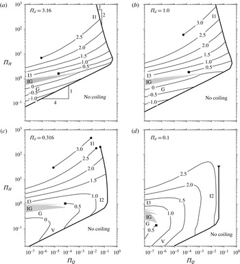
Contour plots of the dimensionless coiling frequency
 $\unicode[STIX]{x1D6F1}_{\unicode[STIX]{x1D6FA}}$
as a function of
 $\unicode[STIX]{x1D6F1}_{Q}$
and
 $\unicode[STIX]{x1D6F1}_{H}$
for four values of
 $\unicode[STIX]{x1D6F1}_{d}$
, determined numerically using the method of Ribe (Reference Ribe2004). The labels on the contours are
 $\log _{10}\unicode[STIX]{x1D6F1}_{\unicode[STIX]{x1D6FA}}$
. Black circles indicate where convergence of the numerical algorithm failed, and black squares show where the calculation was stopped deliberately to avoid entering the multivalued regions (grey). The heavy black lines are the critical curves for coiling onset from figure 2. The labels V, G, IG, I1, I2 and I3 indicate roughly where the corresponding coiling modes reside in the regime diagram.

4 Coiling frequency
The frequency of steady coiling can be predicted using the numerical method of Ribe (Reference Ribe2004) for any values of
 $\unicode[STIX]{x1D6F1}_{H}$
and
 $\unicode[STIX]{x1D6F1}_{Q}$
that lie above and to the left of the critical curves of figure 2. Figure 4 shows contour plots of the dimensionless coiling frequency
 $\unicode[STIX]{x1D6F1}_{\unicode[STIX]{x1D6FA}}$
for four values of
 $\unicode[STIX]{x1D6F1}_{d}$
. The heavy line on each plot is the critical curve for coiling onset from figure 2. To make the connection with figure 1(b), note that the curve in that figure (for which
 $\unicode[STIX]{x1D6F1}_{d}=0.272$
) is very similar to a vertical slice at
 $\unicode[STIX]{x1D6F1}_{Q}=3.78\times 10^{-7}$
through figure 4(c) (for which
 $\unicode[STIX]{x1D6F1}_{d}=0.316$
). In figures 4(c) and 4(d), the contours at lower left loop back on themselves, indicating that the frequency passes through a minimum as the fall height
 $H$
is increased. This behaviour, which is also evident in figure 1(b), corresponds to the transition from V coiling (for which
 $\text{d}\unicode[STIX]{x1D6FA}/\text{d}H<0$
) to G coiling (for which
 $\text{d}\unicode[STIX]{x1D6FA}/\text{d}H>0$
). The grey regions in figure 4 correspond to the multivalued IG mode. A typical variation of
 $\unicode[STIX]{x1D6FA}$
as a function of
 $H$
for the IG mode is the portion
 $\unicode[STIX]{x1D6F1}_{H}\in [0.7,1.6]$
of the curve in figure 1(b).
I begin by determining the coiling onset frequency for the four intermediate asymptotic limits of the critical curves indicated in figure 2. As a preliminary, I note that the frequency of inertial coiling has three distinct scaling laws, depending on the magnitude of the gravitational stretching of the tail. All are based on the fundamental scaling law for the frequency of inertial coiling, which is (Mahadevan et al. Reference Mahadevan, Ryu and Samuel2000)
 $$\begin{eqnarray}\unicode[STIX]{x1D6FA}_{I}\sim \left(\frac{Q^{4}}{\unicode[STIX]{x1D708}a_{1}^{10}}\right)^{1/3}.\end{eqnarray}$$
In the first inertial mode, which I call I1, the tail is in free fall and the viscous resistance to stretching is negligible. In this case, the radius
 $a_{1}\sim (Q^{2}/gH)^{1/4}$
, whence (4.1) becomes
 $$\begin{eqnarray}\unicode[STIX]{x1D6FA}_{I}^{(1)}\sim \left(\frac{g^{5}}{\unicode[STIX]{x1D708}^{2}Q^{2}}\right)^{1/6}H^{5/6}.\end{eqnarray}$$
A second inertial mode (I2) has negligible stretching in the tail, so that
 $a_{1}\approx d/2$
. The scaling law for this mode is therefore
 $$\begin{eqnarray}\unicode[STIX]{x1D6FA}_{I}^{(2)}\sim \left(\frac{Q^{4}}{\unicode[STIX]{x1D708}d^{10}}\right)^{1/3}.\end{eqnarray}$$
Finally, in the third inertial mode (I3), the tail is strongly stretched by gravity, but the latter is balanced by the viscous resistance to stretching rather than by inertia. In this case,
 $a_{1}\sim (\unicode[STIX]{x1D708}Q/gH^{2})^{1/2}$
, and (4.1) becomes
 $$\begin{eqnarray}\unicode[STIX]{x1D6FA}_{I}^{(3)}\sim \left(\frac{g^{5}}{\unicode[STIX]{x1D708}^{6}Q}\right)^{1/3}H^{10/3}.\end{eqnarray}$$
As we shall see, these three inertial modes blend smoothly into one another on the regime diagram.
Figure 5 shows the dimensionless coiling frequency
 $\unicode[STIX]{x1D6F1}_{\unicode[STIX]{x1D6FA}}$
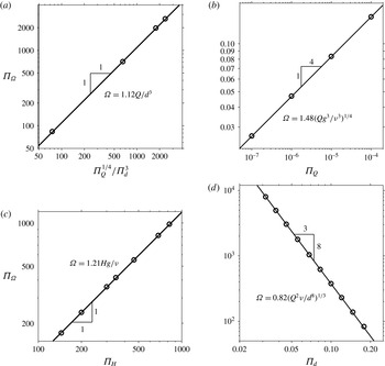
on the critical surface as a function of relevant dimensionless parameters for the four onset modes V (a), G (b), I1 (c) and I2 (d). The dimensional equation for the best-fitting regression line is shown on each panel. As an illustration of how the onset frequency may be written in a more familiar form, consider the mode I1, for which the best-fitting regression line is (in dimensional form)
 $$\begin{eqnarray}\unicode[STIX]{x1D6FA}=1.21Hg/\unicode[STIX]{x1D708}.\end{eqnarray}$$
By using the definition
 $gQ^{2}H/\unicode[STIX]{x1D708}^{4}=2.21$
of the critical surface for this mode, one can rewrite the right-hand side of (4.5) by multiplying it by the unitary quantity
 $(2.21\unicode[STIX]{x1D708}^{4}/gQ^{2}H)^{1/6}$
, whence
 $$\begin{eqnarray}\unicode[STIX]{x1D6FA}=1.21\frac{Hg}{\unicode[STIX]{x1D708}}\left(\frac{2.21\unicode[STIX]{x1D708}^{4}}{gQ^{2}H}\right)^{1/6}=1.38\left(\frac{g^{5}}{\unicode[STIX]{x1D708}^{2}Q^{2}}\right)^{1/6}H^{5/6}.\end{eqnarray}$$
Comparison of (4.6) with (4.2) shows that the onset of coiling along the portion of the critical curve defined by
 $gQ^{2}H/\unicode[STIX]{x1D708}^{4}=2.21$
does indeed correspond to the I1 mode of inertial coiling.
Dimensionless coiling frequency
 $\unicode[STIX]{x1D6F1}_{\unicode[STIX]{x1D6FA}}$
on the critical surface as a function of relevant dimensionless parameters for the four onset modes (a) V, (b) G, (c) I1 and (d) I2. The dimensional form of the best-fitting regression line is indicated on each panel.

A similar analysis applied to the remaining three intermediate asymptotic limits in figure 2 yields scaling laws for the onset frequency for the three additional modes V, G and I2. The results for all four modes are summarized in table 1. The auxiliary conditions in the third column specify where in the parameter space
 $\unicode[STIX]{x1D6F1}_{H}$
–
 $\unicode[STIX]{x1D6F1}_{Q}$
–
 $\unicode[STIX]{x1D6F1}_{d}$
each of the onset criteria applies.
Onset of coiling: asymptotic limits.

With the above results in hand, it is now possible to construct a complete regime diagram for liquid rope coiling. This diagram is just the set of four contour plots of figure 4, with the coiling modes corresponding to the different regions now indicated. The desired synoptic portrait of the ‘whole elephant’ is thus complete.
5 Discussion
Perhaps surprisingly for a phenomenon that has been so extensively studied, the complete regime diagram for liquid rope coiling has not been determined until now. In this study, the regime diagram was constructed as a set of contour plots of the dimensionless coiling frequency
 $\unicode[STIX]{x1D6F1}_{\unicode[STIX]{x1D6FA}}$
as a function of the dimensionless fall height
 $\unicode[STIX]{x1D6F1}_{H}$
and flow rate
 $\unicode[STIX]{x1D6F1}_{Q}$
for several values of the dimensionless nozzle diameter
 $\unicode[STIX]{x1D6F1}_{d}$
. The ensemble of these plots allows the coiling frequency to be predicted as a function of the fall height
 $H$
, the flow rate
 $Q$
, the viscosity
 $\unicode[STIX]{x1D708}$
and the nozzle diameter
 $d$
. The regime diagram should therefore be of interest to researchers working with liquid rope coiling in practical situations ranging from fibre laydown in non-woven textile production to 3D printing.
An interesting feature of the regime diagram is the presence of three distinct varieties of the inertial mode, which differ according to the amount of gravitational stretching in the tail. In particular, that stretching is negligible in mode I2, and the corresponding portion of the regime diagram is here identified for the first time. The mode I3 differs from I1 and I2 in that it is not an onset mode, but only exists in the interior of the regime diagram, well away from the critical onset surface. The same is true of the multivalued IG mode.
The work presented here corrects a small error in Habibi et al. (Reference Habibi, Rahmani, Bonn and Ribe2010), who proposed onset criteria (but not onset frequencies) for the three modes V, G and I1. Instead of the correct onset criterion
 $a_{1}=R$
, these authors determined the locus of points where the numerical solutions exhibit a turning point or fold as the ratio
 $a_{1}/R$
increases. Because the jet is parameterized by arclength, there is nothing to prevent it from intersecting itself numerically, and indeed it is found that steady solutions can exist up to approximately
 $a_{1}/R=1.95$
before the turning point is reached. Use of the (mistaken) turning point criterion changes the numerical factors in table 1 by only approximately 5 %–6 %, but nevertheless the correct values determined in the present study should be used.
Turning towards the future, I believe that the principal remaining task is to understand the inertio-gravitational (IG) coiling mode in greater depth. In this mode, the tail of the rope acts as a distributed pendulum which is forced at the bottom by the bending stresses applied by the coil. The tail enters into resonance with the coil when one of its natural frequencies is close to the frequency fixed by the coil. This is manifested in the downward/rightward facing peaks in the curve of frequency versus fall height in figure 1(b), which are classic resonance peaks whose amplitudes are limited by the nonlinear effects of inertia (Ribe et al. Reference Ribe, Huppert, Hallworth, Habibi and Bonn2006b ). I understand that two colleagues are currently carrying out an analytical study of this complicated behaviour, and I look forward eagerly to their results.
Acknowledgements
This research was supported in part by a grant from the SEDIT program of the institute INSU of the CNRS. I thank three anonymous referees for constructive comments which helped to improve the original paper.