
1. Introduction
Taylor–Couette flow (TCF), the flow between two concentric and independently rotating cylinders, is one of the canonical problems in fluid mechanics, and a paradigm for the study of linear stability, pattern formation and rotationally driven turbulence. From the original investigations of Taylor (Reference Taylor1923) to the pioneering experiments of Coles (Reference Coles1965), recent theoretical analyses (Jones Reference Jones1981; Gebhardt & Grossmann Reference Gebhardt and Grossmann1993; Maretzke, Hof & Avila Reference Maretzke, Hof and Avila2014), high-Reynolds-number simulations (Ostilla et al. Reference Ostilla, Stevens, Grossmann, Verzicco and Lohse2013; Ostilla-Mónico et al. Reference Ostilla-Mónico, van der Poel, Verzicco, Grossmann and Lohse2014; Grossmann, Lohse & Sun Reference Grossmann, Lohse and Sun2016; Sacco, Verzicco & Ostilla-Mónico Reference Sacco, Verzicco and Ostilla-Mónico2019), and experimental investigation (van Gils et al. Reference van Gils, Bruggert, Lathrop, Sun and Lohse2011, Reference van Gils, Huisman, Grossmann, Sun and Lohse2012; Huisman et al. Reference Huisman, van der Veen, Sun and Lohse2014), TCF has remained a problem of interest for most of the last century. Perhaps the most well-known characteristic of TCF is the incredibly rich array of stable flow states that exist over a range of geometries and relative rotation rates of the inner and outer cylinders (Coles Reference Coles1965; Andereck, Liu & Swinney Reference Andereck, Liu and Swinney1986). We consider the case of pure inner cylinder rotation, for which the problem is parametrized by the ratio of the inner and outer radii,  $\eta \equiv r_i/r_o$, and a single Reynolds number,
 $R$. In this case the laminar velocity profile becomes linearly unstable at a critical Reynolds number,
 $R_c \sim {O} (10^{2})$. A centrifugal instability leads to the formation of a periodic array of toroidal vortex structures known as Taylor vortices or Taylor rolls. For a given geometry, these steady, axisymmetric Taylor vortices are stable and exist for some range of Reynolds number in what is known as the Taylor vortex flow (TVF) regime. As the rotation rate of the inner cylinder is increased further, the Taylor vortices experience a secondary instability giving rise to azimuthally travelling waves whose phase speed is determined by the geometry but whose azimuthal periodicity is not unique (Coles Reference Coles1965). This regime is known as wavy vortex flow (WVF) and is characterized by being time periodic in a stationary reference frame but steady in a frame corotating with the travelling wave (Marcus Reference Marcus1984). WVF is again stable for some range of Reynolds numbers before the travelling waves themselves become unstable, and a second temporal frequency arises causing the travelling waves to become modulated in space and time in what is known as modulated wavy vortex flow (MWVF). As the driving of the inner cylinder is increased further still, the flow becomes disordered and begins to transition to turbulence. However, while the main sequence of transitions from laminar flow to the bifurcation to TVF at
 $R_c \approx 100$, to WVF, to MWVF, and finally on to turbulence at
 $R \approx 1000$ occurs over a relatively narrow range of Reynolds numbers, the large-scale Taylor vortices are present up to
 $R \sim {O} (10^{5})$ (Grossmann et al. Reference Grossmann, Lohse and Sun2016).
In recent years there has been renewed interest (Dessup et al. Reference Dessup, Tuckerman, Wesfreid, Barkley and Willis2018; Sacco et al. Reference Sacco, Verzicco and Ostilla-Mónico2019) in the dynamics of TVF and WVF as a model system to study the self-sustaining process (SSP) proposed by Waleffe (Reference Waleffe1997). The SSP consists of streamwise rolls that advect the mean shear giving rise to streaks of streamwise velocity, which become unstable to wave-like disturbances, which in turn nonlinearly interact to sustain the rolls (Hamilton, Kim & Waleffe Reference Hamilton, Kim and Waleffe1995; Waleffe Reference Waleffe1997). Dessup et al. (Reference Dessup, Tuckerman, Wesfreid, Barkley and Willis2018) performed direct numerical simulations (DNSs) to show that the mechanism of transition from TVF to WVF follows the same path as described in the SSP: the travelling waves of WVF arise from an instability of the streamwise velocity component (streaks) of TVF with the cross-stream velocity (rolls) playing a negligible role in the instability mechanism. Sacco et al. (Reference Sacco, Verzicco and Ostilla-Mónico2019) extended this line of study to higher Reynolds numbers and showed that despite their origin as a centrifugal instability, turbulent Taylor vortices are preserved in the limit of vanishing curvature and are thus not dependent on rotational effects, but rather are sustained through a nonlinear feedback loop between the rolls and streaks.
The SSP is believed to be one of the building blocks of turbulence and thus the study of self-sustaining solutions of the Navier–Stokes equations (NSEs), known as exact coherent states (ECSs), has been of great interest to researchers since they were first discovered by Nagata (Reference Nagata1990). The field has grown immensely in the intervening years and we make no attempt to summarize it all here. Of primary interest is the observation that many of these solutions resemble streamwise elongated vortices and streaks, and thus resemble structures observed in experiments and simulations of turbulent flows (Beaume et al. Reference Beaume, Chini, Julien and Knobloch2015). This has led to the idea that ECSs make up the phase space skeleton of turbulence, and that the observation of these structures indicates the turbulent trajectory passing by one of these ECS solutions.
Due to the significant mathematical simplification, it is useful to model these elongated structures as being infinitely long in their streamwise extent. Illingworth (Reference Illingworth2020) studied the linear amplification mechanism of such streamwise invariant structures to identify the most amplified spanwise length scales in both channel and plane Couette flow (PCF), and found that the latter was far more efficient in amplifying these structures. However, no structures actually observed in channel or plane Couette flow are truly invariant in the streamwise direction. Additionally, ECSs are generally unstable; while the turbulent trajectory may visit these states, they do not actually persist in nature. TVF is thus a valuable test case to study the nonlinear dynamics sustaining ECSs in general since it is in fact a stable solution observed in experiment and due to the cylindrical geometry is exactly streamwise constant.
We aim to help bridge the gap between linear stability theory, which accurately predicts the genesis of Taylor vortices, and higher Reynolds numbers where Taylor vortices are sustained by fully nonlinear mechanisms as shown by Sacco et al. (Reference Sacco, Verzicco and Ostilla-Mónico2019). The resolvent formulation of the NSE, which interprets the nonlinear term in the NSE as a forcing to the linear dynamics, offers a natural path from linear to nonlinear analysis and as such will form the basis of our modelling efforts. Resolvent analysis has historically been successful in exploiting the linear dynamics to identify structures in turbulence, which is by nature a nonlinear phenomenon (McKeon & Sharma Reference McKeon and Sharma2010). However, recent attempts have been made to explicitly characterize and quantify the influence of nonlinear dynamics within the resolvent framework. For example, Moarref et al. (Reference Moarref, Jovanović, Tropp, Sharma and McKeon2014) and McMullen, Rosenberg & McKeon (Reference McMullen, Rosenberg and McKeon2020) used convex optimization to compute reduced-order representations of turbulent statistics and Rigas, Sipp & Colonius (Reference Rigas, Sipp and Colonius2021) studied solutions of the harmonic-balanced NSEs to identify optimal nonlinear mechanisms leading to boundary layer transition. Additionally Morra et al. (Reference Morra, Nogueira, Cavalieri and Henningson2021) and Nogueira et al. (Reference Nogueira, Morra, Martini, Cavalieri and Henningson2021) have directly computed the nonlinear forcing statistics for minimal channel and Couette flow respectively, and analysed the efficacy of low-rank resolvent reconstructions in capturing the relevant dynamics.
In this work we use optimization-based methods not only to capture statistics, but to explicitly model the self-sustaining nonlinear system. To the best of these authors’ knowledge this work is the first example in the literature of ‘closing the resolvent loop’ where the feedback loop formulation of the NSE introduced by McKeon & Sharma (Reference McKeon and Sharma2010) is used to generate solutions to the fully nonlinear NSE.
In § 2 we outline the resolvent formulation of the NSE and our optimization-based model. In § 3 we present the results of our model, compare them with DNS and present a detailed analysis of the nonlinear dynamics. We discuss applications of our results to DNS of turbulent TCF in § 4 and conclude with some final remarks in § 5.
2. Mathematical description
We study the flow of an incompressible Newtonian fluid with kinematic viscosity  $\nu$ between two concentric cylinders using the NSE in cylindrical coordinates,
 \begin{gather} \frac{\partial \tilde{\boldsymbol{u}}}{\partial t} + \tilde{\boldsymbol{u}} \boldsymbol{\cdot}\boldsymbol{\nabla} \tilde{\boldsymbol{u}} - \frac{1}{R}\nabla^{2} \tilde{\boldsymbol{u}} -\boldsymbol{\nabla} \tilde{p} = 0, \end{gather}
 \begin{gather}\boldsymbol{\nabla} \boldsymbol{\cdot} \tilde{\boldsymbol{u}}=0, \end{gather}
on the domain  $r\in [r_i,r_o]$,
 $\theta \in [0, 2{\rm \pi} ]$,
 $z\in [-L_z/2,L_z/2]$. We will consider the case where the outer cylinder is held fixed while the inner cylinder rotates with a prescribed azimuthal speed
 $U_i$. The equations are non-dimensionalized using the gap width
 $d\equiv r_o-r_i$ and the azimuthal velocity of the inner cylinder
 $U_i$. The Reynolds number is defined as
 $R\equiv U_i d/\nu$. In these non-dimensional variables the limits of the radial domain are given as a function of the radius ratio
 $\eta$ by
 $r_i=\eta /(1-\eta )$ and
 $r_o = 1/(1-\eta )$. Throughout this work we fix
 $\eta = 0.714$, for which the critical Reynolds number
 $R_c = 81$. This
 $\eta$ was chosen to allow for comparison to past studies, such as those of Ostilla et al. (Reference Ostilla, Stevens, Grossmann, Verzicco and Lohse2013), and since it allows for a larger range of Reynolds numbers for which TVF is a stable solution of (2.1).
We decompose the state  $[\tilde {\boldsymbol {u}},\tilde {p}]=[\tilde {u}_r,\tilde {u}_\theta ,\tilde {u}_z,p]$ into a mean and fluctuating component,
 \begin{equation} [\tilde{\boldsymbol{u}}(r,z,\theta,t),\tilde{p}(r,z,\theta,t)] = [ \bar{\boldsymbol{U}}(r),\bar{P}(r)] + [\boldsymbol{u}(r,z,\theta,t),p(r,z,\theta,t)], \end{equation}
with
 \begin{equation} \bar{({\cdot})}\equiv \lim_{T,L\to\infty} \frac{1}{2{\rm \pi} T L} \int_{0}^{T}\int_{0}^{2{\rm \pi}}\int_{0}^{L} ({\cdot})\,\textrm{d}z\, \textrm{d}\theta\, \textrm{d}t, \end{equation}
which upon substitution into (2.1), and averaging over  $z, \theta$ and
 $t$ results in the mean momentum equation
 $$\begin{gather} \bar{\boldsymbol{U}} \boldsymbol{\cdot}\boldsymbol{\nabla} \bar{\boldsymbol{U}} - \frac{1}{R}\nabla^{2} \bar{\boldsymbol{U}} -\boldsymbol{\nabla} \bar{P} ={-}\overline{\boldsymbol{u} \boldsymbol{\cdot}\boldsymbol{\nabla} \boldsymbol{u}}, \end{gather}$$
 $$\begin{gather}\boldsymbol{\nabla} \boldsymbol{\cdot} \bar{\boldsymbol{U}} = 0. \end{gather}$$
Subtracting (2.5) from the full NSE then results in a governing equation for the fluctuations, where we have grouped those terms which are nonlinear in the fluctuations on the right-hand side in anticipation of the following analysis:
 \begin{gather} \frac{\partial \boldsymbol{u}}{\partial t} + \bar{\boldsymbol{U}} \boldsymbol{\cdot}\boldsymbol{\nabla} \boldsymbol{u} + \boldsymbol{u} \boldsymbol{\cdot}\boldsymbol{\nabla} \bar{\boldsymbol{U}}- \frac{1}{R}\nabla^{2} \boldsymbol{u} -\boldsymbol{\nabla} p ={-}(\boldsymbol{u} \boldsymbol{\cdot}\boldsymbol{\nabla} \boldsymbol{u}-\overline{\boldsymbol{u} \boldsymbol{\cdot}\boldsymbol{\nabla} \boldsymbol{u}}), \end{gather}
 \begin{gather}\boldsymbol{\nabla} \boldsymbol{\cdot} \boldsymbol{u} = 0 \end{gather}
 \begin{gather}\bar{\boldsymbol{U}}|_{r_i} = \hat{e}_{\theta}, \quad \bar{\boldsymbol{U}}|_{r_o} = \boldsymbol{u}|_{r_i}=\boldsymbol{u}|_{r_o} = \boldsymbol{0}. \end{gather}
2.1. Direct numerical simulation
In order to validate our model solution we perform DNS of TCF for a range of Reynolds number,  $100< R<2000$, for a radius ratio
 $\eta = 0.714$ and an aspect ratio
 $L_z/d = 12$. However, our analysis is focused primarily on the cases
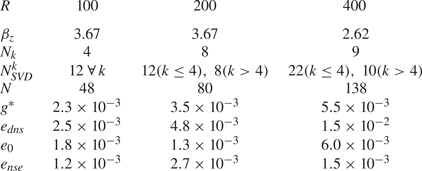
 $R = 100$, 200 and 400. The details of the numerical method can be found in the papers by Verzicco & Orlandi (Reference Verzicco and Orlandi1996), van der Poel et al. (Reference van der Poel, Ostilla-Mónico, Donners and Verzicco2015) and Zhu et al. (Reference Zhu2018), and the details of the simulations performed in this work are summarized in table 1.
Numerical details of DNS. Note: DOF, degrees of freedom.

2.2. Resolvent analysis
Our model solution will be based on the resolvent formulation of McKeon & Sharma (Reference McKeon and Sharma2010), which assumes that the one-dimensional mean velocity profile  $\bar {\boldsymbol {U}}(r)$ is known. This allows us to write (2.7) and (2.8) as a balance between the linear dynamics and the nonlinear term which we group into a forcing term denoted by
 $\boldsymbol {f}$:
 \begin{equation} \mathcal{L}\boldsymbol{u}=\mathcal{N}(\boldsymbol{u},\boldsymbol{u}) \equiv \boldsymbol{f}. \end{equation}
For notational simplicity we define the state  $\boldsymbol {u}$ to include both the three components of velocity,
 $[u_r,u_{\theta },u_z]$ as well as the pressure
 $p$. We then Fourier transform the state
 $\boldsymbol {u}(r,z,\theta ,t)$ and the nonlinear forcing
 $\boldsymbol {f}(r,z,\theta ,t)$ in time as well as in the homogeneous spatial directions,
 $z$ and
 $\theta$. For a function
 $\boldsymbol {q}(r,z,\theta ,t)$ the Fourier transform is defined as
 \begin{equation} \hat{\boldsymbol{q}}(r,k,n,\omega)\equiv \int_{-\infty}^{\infty}\int_{\infty}^{\infty}\int_{0}^{2{\rm \pi}} \boldsymbol{q}(r,z,\theta,t)\,\textrm{e}^{-\textrm{i}(k_z z +n\theta -\omega t) }\,\textrm{d}\theta\, \textrm{d}z\, \textrm{d}t. \end{equation}
This results in a system of coupled ordinary differential equations (ODEs) for the Fourier modes  $\hat {\boldsymbol {u}}_{\boldsymbol {k}}(r)$ and
 $\hat {\boldsymbol {f}}_{\boldsymbol {k}}(r)$ parametrized by the wavenumber triplet
 $\boldsymbol {k}\equiv [k_z,n,\omega ]$. The domain is periodic in the azimuthal direction and we formally consider the case
 $L_z = \infty$, so we have
 $n \in \mathbb {Z}$ and
 $k_z,\omega \in \mathbb {R}$:
 \begin{equation} (\mathcal{L}_{\boldsymbol{k}}-\textrm{i}\omega {\boldsymbol{\mathsf{M}}}) \hat{\boldsymbol{u}}_{\boldsymbol{k}} =\hat{\boldsymbol{f}}_{\boldsymbol{k}}. \end{equation}
The explicit expressions for the Fourier transformed linear operator  $\mathcal {L}_{\boldsymbol {k}}$ and the weight matrix
 ${\boldsymbol{\mathsf{M}}}$ are given in Appendix A. If we then invert the linear operator on the left-hand side of (2.12), we arrive at the characteristic input-output representation of the NSE of McKeon & Sharma (Reference McKeon and Sharma2010) where the linear dynamics represents a transfer function from the nonlinearity, which is interpreted as a forcing, and the velocity:
 \begin{equation} \hat{\boldsymbol{u}}_{\boldsymbol{k}} = (\mathcal{L}_{\boldsymbol{k}} - \textrm{i}\omega {\boldsymbol{\mathsf{M}}})^{{-}1}\hat{\boldsymbol{f}}_{\boldsymbol{k}}. \end{equation}
A singular value decomposition (SVD) of this transfer function, which we call the resolvent and denote by  $\mathcal {H}$, provides an orthonormal basis for the velocity as well as the forcing, where superscript
 $H$ denotes the conjugate transpose:
 \begin{equation} \mathcal{H}_{\boldsymbol{k}} \equiv (\mathcal{L}_{\boldsymbol{k}} - \textrm{i}\omega {\boldsymbol{\mathsf{M}}})^{{-}1} = \varPsi_{\boldsymbol{k}} \varSigma_{\boldsymbol{k}} \varPhi_{\boldsymbol{k}}^{H}. \end{equation}
The columns of  $\varPsi _{\boldsymbol {k}}$ and
 $\varPhi _{\boldsymbol {k}}$, denoted by
 $\boldsymbol {\psi }_{\boldsymbol {k},j}$ and
 $\boldsymbol {\phi }_{\boldsymbol {k},j}$, are referred to as the resolvent response and forcing modes respectively and are ordered by their singular values
 $\sigma _{\boldsymbol {k},j}$ such that
 $\sigma _{\boldsymbol {k},1}\geq \sigma _{\boldsymbol {k},2}\geq \cdots \geq \sigma _{\boldsymbol {k},j}\geq \sigma _{\boldsymbol {k},j+1}$. Thus
 $\boldsymbol {\psi }_{\boldsymbol {k},1}$ represents the most linearly amplified structure at that wavenumber. Note that these modes are vector fields over
 $r$ which are orthonormal with respect to an
 $L_2$ inner product over the three velocity components
 \begin{equation} \langle \boldsymbol{a},\boldsymbol{b}\rangle \equiv \int_{r_i}^{r_o} a^{*}_m(r)b_m(r) r\, \textrm{d}r, \end{equation}
with associated norm
 \begin{equation} \|\boldsymbol{a}\|\equiv \langle \boldsymbol{a},\boldsymbol{a}\rangle^{1/2}, \end{equation}
where summation over  $m$ is implied, such that
 \begin{equation} \langle \boldsymbol{\psi}_{\boldsymbol{k},i},\boldsymbol{\psi}_{\boldsymbol{k},j} \rangle = \langle \boldsymbol{\phi}_{\boldsymbol{k},i},\boldsymbol{\phi}_{\boldsymbol{k},j} \rangle = \delta_{ij}. \end{equation}
In this resolvent basis, each Fourier mode of the velocity and forcing may be written as
 \begin{gather} \hat{\boldsymbol{u}}_{\boldsymbol{k}} = \sum_{j=1}^{\infty} \sigma_{\boldsymbol{k},j} \chi_{\boldsymbol{k},j} \boldsymbol{\psi}_{\boldsymbol{k},j}, \end{gather}
 \begin{gather}\hat{\boldsymbol{f}}_{\boldsymbol{k}} = \sum_{j=1}^{\infty} \chi_{\boldsymbol{k},j} \boldsymbol{\phi}_{\boldsymbol{k},j}, \end{gather}
where  $\chi _{\boldsymbol {k},j} \equiv \langle \phi _{\boldsymbol {k},j} ,\hat {\boldsymbol {f}}_{\boldsymbol {k}} \rangle$ represents the projection of the (unknown) forcing onto the forcing modes.
2.3. Symmetries of Taylor vortex flow
The various flow states observed in TCF (TVF, WVF and MWVF) may be defined by their spatiotemporal symmetries (Rand Reference Rand1982). We define TVF, the focus of this study, as a solution to (2.1) which is steady, axisymmetric and axially periodic with fundamental wavenumber  $\beta _z$, meaning we restrict ourselves to wavenumber vectors of the form
 $\boldsymbol {k}=[k_z,n,\omega ] = [k\beta _z,0,0]$ where
 $k\in \mathbb {Z}$. This fundamental wavenumber
 $\beta _z$ is related to the axial height of the Taylor vortices and is generally constrained by the experimental apparatus or computational box since the domain must contain an integer number of vortices. The resolvent formulation assumes an infinite axial domain so the choice of
 $\beta _z$ is not immediately obvious. However, we found that the results shown in this work are robust to changes in
 $\beta _z$ as long as
 ${\rm \pi} /2 \lesssim \beta _z \lesssim 4{\rm \pi} /3$. Therefore, we choose the axial periodicity of our model to match that observed in our DNS, allowing for a direct comparison between our model and the DNS. The specific values of
 $\beta _z$ are listed in table 2. Given these symmetries, our model solution will consist of an expansion in Fourier modes:
 \begin{equation} \boldsymbol{u}(r,z) = \sum_{k=1}^{N_k} \hat{\boldsymbol{u}}_k(r)\,\textrm{e}^{\textrm{i} k\beta_z z} + \textrm{c.c.}, \end{equation}
where each Fourier mode  $\hat {\boldsymbol {u}}_k$ is itself an expansion in resolvent modes given by (2.18) and c.c. denotes the complex conjugate. We truncate the model at
 $N_k$ Fourier modes each of which is expanded in
 $N^{k}_{SVD}$ resolvent modes such that the final form of the TVF solution is given by
 \begin{equation} \boldsymbol{u}(r,z) = \sum_{k=1}^{N_k}\sum_{j=1}^{N^{k}_{SVD}} \sigma_{k,j} \chi_{k,j} \boldsymbol{\psi}_{k,j}(r)\,\textrm{e}^{\textrm{i} k\beta_z z} + \textrm{c.c.} \end{equation}


2.4. Treatment of the nonlinearity
At any given wavenumber, the forcing  $\hat {\boldsymbol {f}}_{k}$ is given by a convolution sum of the interactions of all triadically compatible velocity modes:
 \begin{equation} \hat{\boldsymbol{f}}_k={-}\sum_{m\neq 0} \sum_{n\neq 0} (\hat{\boldsymbol{u}}_{m}\boldsymbol{\cdot} \boldsymbol{\nabla} \hat{\boldsymbol{u}}_{n})\delta_{m+n,k}. \end{equation}
Here  $\delta _{a,b}$ is the Kronecker delta which implies that the forcing at a given wavenumber
 $k$ contains only interactions between Fourier modes whose wavenumbers sum to
 $k$. Throughout this work we use the terminology ‘
 $k_1 = k_2 + k_3$’ to refer to a single (resonant) triad involving the nonlinear interaction between Fourier modes with wavenumbers
 $k_2$ and
 $k_3$ forcing the Fourier mode with wavenumber
 $k_1$.
Equating the two expressions for the forcing mode given by (2.19) and (2.22) and substituting (2.18) for the velocity modes gives
 \begin{equation} \sum_{j=1}^{\infty} \chi_{k,j} \boldsymbol{\phi}_{k,j} =\sum_{m\neq 0} \sum_{n\neq 0} \sum_{p=1}^{\infty} \sum_{q=1}^{\infty}- \chi_{m,p} \chi_{n,q} \sigma_{m,p} \sigma_{n,q}(\boldsymbol{\psi}_{m,p}\boldsymbol{\cdot} \boldsymbol{\nabla} \boldsymbol{\psi}_{n,q})\delta_{m+n,k}. \end{equation}
Projecting both sides of (2.23) onto each forcing  $\boldsymbol {\phi }_{k,i}$ and dropping the summation symbols for simplicity gives
 \begin{equation} \chi_{k,i} = \chi_{m,p} \chi_{n,q} N_{kmn,ipq}, \end{equation}
where the  $N_{kmn,ipq}$ are called the interaction coefficients and are given by
 \begin{equation} N_{kmn,ipq} \equiv{-} \sigma_{m,p} \sigma_{n,q} \langle \boldsymbol{\phi}_{k,i},(\boldsymbol{\psi}_{m,p}\boldsymbol{\cdot} \boldsymbol{\nabla} \boldsymbol{\psi}_{n,q})\rangle\delta_{m+n,k}, \end{equation}
which, critically, can be computed solely from knowledge of the linear operator  $\mathcal {H}$.
Nonlinear interactions between the velocity fluctuations also appear in the divergence of the Reynolds stress on the right-hand side of (2.5). This term is referred to as the ‘mean forcing’ and is given by the sum of nonlinear interactions of all the  $\hat {\boldsymbol {u}}_k$ and their complex conjugates
 $\hat {\boldsymbol {u}}_{-k}$, which can be directly interpreted as (2.22) evaluated at
 $k = {0}$:
 \begin{equation} \overline{\boldsymbol{u} \boldsymbol{\cdot}\boldsymbol{\nabla} \boldsymbol{u}} = \sum_{k\neq \boldsymbol{0}} (\hat{\boldsymbol{u}}_{k}\boldsymbol{\cdot}\boldsymbol{\nabla} \hat{\boldsymbol{u}}_{{-}k} + \hat{\boldsymbol{u}}_{{-}k}\boldsymbol{\cdot}\boldsymbol{\nabla} \hat{\boldsymbol{u}}_{k} ). \end{equation}
At this point we would like to reiterate that the mean velocity profile is assumed to be known a priori. Thus the left-hand side of (2.5), and therefore the Reynolds stress divergence on the left-hand side of (2.26), is also known.
We have thus reduced the NSE (under the assumption of a known mean velocity) to the infinite system of coupled polynomial equations (2.24) for the complex coefficients  $\chi _{\boldsymbol {k},j}$ with the auxiliary condition that (2.26) is satisfied. While deriving an exact (non-trivial) solution to (2.24) may be a daunting task, we will demonstrate that approximate solutions can be efficiently computed by minimizing the residuals associated with (2.24) and (2.26).
2.5. Optimization problem
We have recast the NSE in the language of resolvent analysis as
 \begin{gather} \chi_{k,j} - \chi_{m,p} \chi_{n,q} N_{kmn,jpq} = 0,\quad \forall \, k,j \end{gather}
 \begin{gather}\overline{\boldsymbol{u} \boldsymbol{\cdot}\boldsymbol{\nabla} \boldsymbol{u}} - \boldsymbol{f}_{0,k',pq} \chi_{k',p} \chi^{*}_{k',q} = \boldsymbol{0}, \end{gather}
 \begin{gather}\boldsymbol{f}_{0,k,pq} \equiv \sigma_{k,p} \sigma_{k,q}(\hat{\boldsymbol{\psi}}_{k,p}\boldsymbol{\cdot} \boldsymbol{\nabla} \hat{\boldsymbol{\psi}}^{*}_{k,q} + \hat{\boldsymbol{\psi}}_{k,q}^{*}\boldsymbol{\cdot} \boldsymbol{\nabla} \hat{\boldsymbol{\psi}}_{k,p}), \end{gather}
where we have expanded the velocity Fourier modes in their resolvent basis according to (2.18), and summation over  $m, n$ and
 $k'$ is implied. We truncate the expansion at some number of harmonics,
 $N_k$, of the fundamental wavenumber, and at each retained harmonic we truncate the singular mode expansion at
 $N^{k}_{SVD}$ such that the total number of retained modes is
 $N=\sum ^{N_k}_{k=1}N^{k}_{SVD}$. We seek to minimize the residuals (in the sense of the
 $L_2$ norm) associated with (2.27) and (2.28), and thus formulate the following optimization problem:
 \begin{equation} \min_{\chi_{k,j}} g^{2}(\chi_{k,j}) = a g^{2}_0(\chi_{k,j}) + (1-a) g^{2}_{triad}(\chi_{k,j}). \end{equation}
The first and second terms on the right-hand side in (2.30) are defined as the mean constraint,
 \begin{equation} g_0(\chi_{k,j}) \equiv \frac{\|\overline{\boldsymbol{u} \boldsymbol{\cdot}\boldsymbol{\nabla} \boldsymbol{u}} -\boldsymbol{f}_{0,k',p q} \chi_{k',p} \chi_{k',q}^{*}\|}{\|\overline{\boldsymbol{u} \boldsymbol{\cdot}\boldsymbol{\nabla} \boldsymbol{u}}\|} \end{equation}
and the triadic constraint,
 \begin{equation} g_{triad}(\chi_{k,j}) \equiv |\chi_{k,j} - \chi_{m,p} \chi_{n,q} N_{kmn,jpq}|. \end{equation}
The former represents the residual in the mean momentum equation (2.5), while the latter represents the residual in the equation for the fluctuations (2.7). The user-defined weighting parameter  $a\in (0,1)$ determines the relative penalization of each of these two constraints in the residual.
At this point we would like to highlight several important aspects of problem (2.30). First, we reiterate that the left-hand term in the mean constraint equation (2.31) is a known function since the mean velocity profile is assumed to be known a priori. Second, we emphasize that we have assumed no closure model and made no modelling assumptions regarding the form of the nonlinear forcing in the derivation of (2.30). Lastly, while in general the amplitudes  $\chi _{k,j} \in \mathbb {C}$, for the special case of steady, axially periodic and axisymmetric solutions considered here, evaluating (2.12) and (A1) for
 ${\pm }k$ reveals that
 $\chi _{k,j} \in \mathbb {R} \ \forall \, j,k$ meaning the optimization need only be carried out over a real valued domain. Note that if this method were applied to non-axially periodic solutions one would have to consider complex coefficients.
Finally, we note that while the reformulation of the NSE (2.7) in the resolvent framework (2.27) is reminiscent of a Galerkin method (GM) where the governing equations are projected onto some predetermined set of basis functions, the current approach is appreciably different. Since we consider a steady process we can not integrate the equations forward in time as would be generally done in the GM. Furthermore, since the resolvent framework provides a basis for both the velocity and the nonlinearity, (2.27) is an exact representation of (2.7) whereas the GM represents the governing equations only in an integral sense.
2.6. Solution methodology
We solve the optimization problem (2.30) using a trust-region algorithm built into Matlab's  $fminunc$ function for
 $R = 100$, 200 and 400. For each Reynolds number the mean velocity profile used in constructing (2.14) is taken from the DNS described in § 2.1. We note that various authors, such as Mantič-Lugo, Arratia & Gallaire (Reference Mantič-Lugo, Arratia and Gallaire2014, Reference Mantič-Lugo, Arratia and Gallaire2015), Rosenberg & McKeon (Reference Rosenberg and McKeon2019a) and Bengana & Tuckerman (Reference Bengana and Tuckerman2021), have computed approximate mean velocity profiles from the laminar base flow for a range of flows. These methods approximate the Reynolds stress as the self-interaction of a single eigen- or resolvent mode. However, we note that Bengana & Tuckerman (Reference Bengana and Tuckerman2021) have described conditions under which such approximations are expected to fail. We do not employ such methods here, choosing instead to focus on the prediction of the velocity fluctuations about a known mean flow.
The gradient and Hessian of (2.30) may be derived explicitly and are input to the algorithm to improve accuracy. The weighting parameter  $a$ in (2.30) is set to 0.01 which means that the triadic constraint is penalized 99 times more heavily than the mean constraint. This reflects the observation that the triadic constraint which encodes the fully nonlinear governing equation for the fluctuations is far more complex than the mean constraint which, given the fact that the mean profile is known, is simply a least-squares fit to a curve.
While this value of  $a$ was found to lead to the most consistent and accurate results, the results are qualitatively robust to changes in
 $a$ as long as
 $0.0005\lesssim a \lesssim 0.8$. If
 $a\lesssim 0.0005$, i.e. the triadic constraint is weighted too heavily, the optimization converges to the laminar state since the triadic constraint admits a trivial solution. If
 $a\gtrsim 0.8$, the mean constraint is weighted too heavily and the optimization tends to over fit to the input mean. Since the triadic constraint is simply a least-squares fit to a known curve, the error can in principle be reduced arbitrarily with increased degrees of freedom. However, this does not guarantee that the resulting local minimum will represent a realistic solution.
The optimization also requires an initial guess. For this we solve the rank 1 formulation of (2.30) using just one wavenumber, the fundamental, and one resolvent mode, in which case the minimum can be found analytically, which results in an amplitude  $\sigma _{1,1}\chi _{1,1} \approx 0.13$. We then initialize the full optimization such that
 $\sigma _{1,1}\chi _{1,1}=0.13$ and the remaining
 $\sigma _{k,j}\chi _{k,j}$ are assigned random values between
 $-$0.01 and 0.01. This range of initial values was chosen to roughly reflect the expected roll off in the amplitudes
 $\sigma _{k,j}\chi _{k_j}$. However, we did not find any dependence on these initial values as long as these amplitudes were not all set to zero, in which case the optimization tended to converge to the trivial solution.
We assess the convergence and accuracy of our model solution using three metrics. First, we compute the final minimum residual of the cost function in (2.30) denoted  $g^{*}$. Second, we compute the error of the model solution compared with the temporal average of the DNS solution:
 \begin{equation} e_{dns} \equiv \sqrt{ \sum_{k=1}^{N_k} \|\boldsymbol{\hat{u}}_k-\boldsymbol{\hat{u}}_{k,dns}\|^{2}}, \end{equation}
where the norm is defined in (2.16). Third, we quantify the error of our model solution in solving the underlying governing equations (2.7), the details of which are discussed in § 3.2.
We note that the error metric comparing our model with the DNS should be viewed with some caution since the Fourier decomposition of the DNS involves some inherent uncertainty. While our model is formulated in Fourier space, the DNS with which we compare our model utilizes a finite difference method in the axial direction. This means that the five or six Taylor vortices in the computational domain are not necessarily exactly the same size and the fundamental wavenumber  $\beta _z$ can only be defined in an average sense,
 \begin{equation} \beta_z = 2{\rm \pi} \frac{n_{roll}}{L_z}, \end{equation}
where  $n_{roll}$ is the number of Taylor vortices contained in the domain and
 $L_z$ is the axial domain size. We use this average
 $\beta _z$ in the construction of our model. To compute the DNS Fourier modes used in (2.33) we extract a single Taylor vortex whose size is closest to the average and perform a Fourier decomposition on this reduced domain. The largest difference between this best fit wavenumber and the average we observed was
 $0.5\,\%$. Since the radial shape of the Taylor vortices is expected to differ slightly with axial size it is unclear whether minor differences between our results and those from DNS arise from errors in our model or uncertainties in the Fourier decomposition of the DNS.
At  $R=400$, which will be the main focus in this work, it was found that
 $N_k=9$ axial wavenumbers with
 $N^{k}_{SVD} = 22$ for
 $k\leq 4$ and
 $N^{k}_{SVD} = 10$ for
 $k>4$ resolvent modes were sufficient such that we did not observe any further meaningful decrease in the residual
 $g^{*}$ with increased
 $N$. A detailed discussion of the choice of these particular truncation values is presented in § 3.6. These truncation values, the total degrees of freedom, the axial wavenumber
 $\beta _z$, as well as the error metrics for all three Reynolds numbers are summarized in table 2.
3. Results
3.1. Velocity field reconstruction
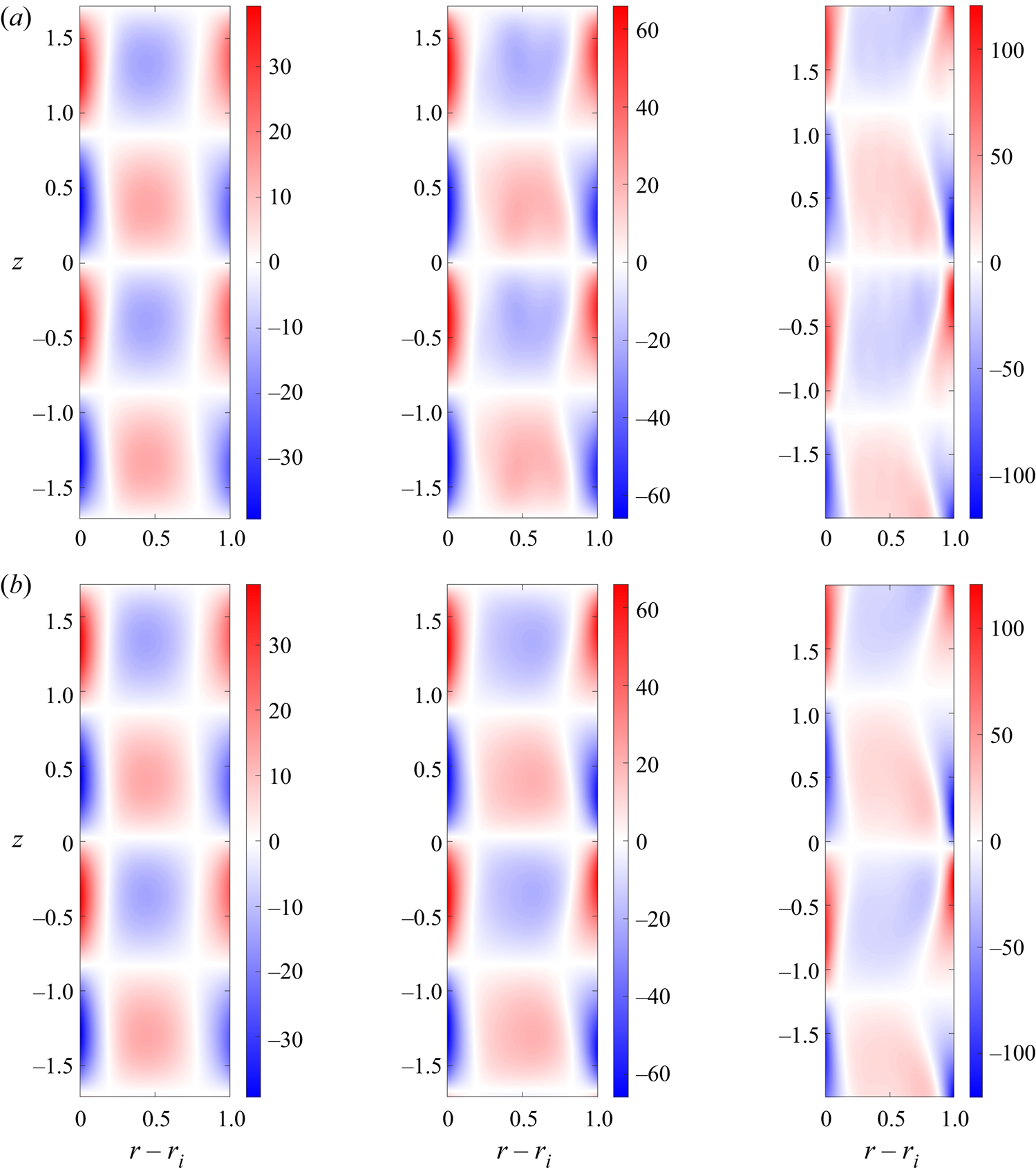
The final result of the model is shown in figures 1 and 2 where we compare the model result with that from DNS. We plot the mean-subtracted azimuthal velocity  $u_{\theta }$ and the azimuthal vorticity
 $\omega _{\theta }={\partial u_r}/{(\partial z)} - {\partial u_z}/{(\partial r)}$ for
 $R=100$, 200 and 400. The model solution is axisymmetric and steady by construction, and thus the radial and axial velocities are linked through continuity; no information is omitted by plotting
 $\omega _{\theta }$. As a comparison we show the azimuthal average of the mean subtracted DNS; however, at this Reynolds number the flow is axisymmetric and steady, so the average field shown is representative of the flow at any azimuthal location and at any instance in time. There is good agreement between the resolvent model (a) and the DNS (b). The model accurately captures the dominant structure of the flow including the strong plumes of azimuthal velocity. The azimuthal vorticity exhibits a chequerboard pattern of regions of roughly constant vorticity of opposing signs. Regions of higher vorticity are concentrated near the walls, while the larger segments in the bulk of the domain have comparatively lower levels of vorticity. These results are in agreement with those obtained from DNS by Sacco et al. (Reference Sacco, Verzicco and Ostilla-Mónico2019), who found that as the Reynolds number increases this concentration of vorticity at the walls is enhanced and the bulk becomes increasingly ‘empty’ of vorticity.
Mean subtracted azimuthal velocity  $u_{\theta }$ computed by our model (a) and DNS (b) at (from left to right)
 $R=100$, 200 and 400.

Azimuthal vorticity  $\omega _{\theta }={\partial u_r}/{(\partial z)} - {\partial u_z}/{(\partial r)}$ computed by our model (a) and DNS (b) at (from left to right)
 $R=100$, 200 and 400.

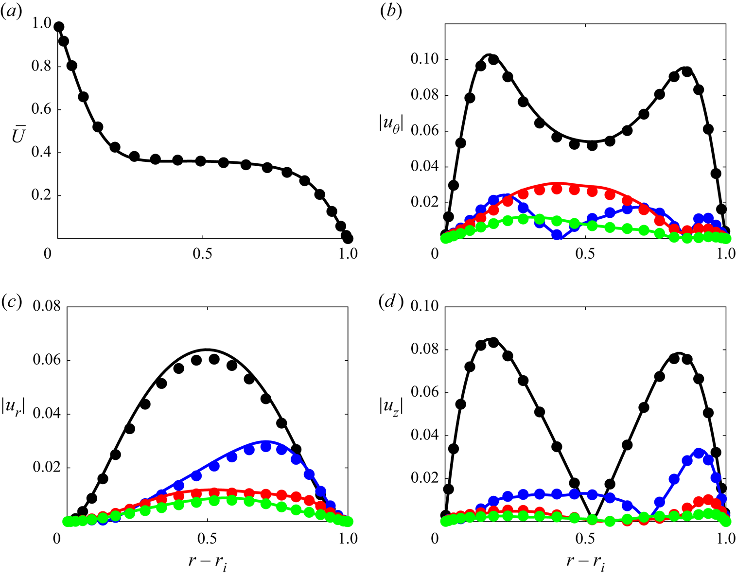
A more quantitative assessment of the model's accuracy is shown in figure 3 where we compare the individual Fourier modes of the model solution with the Fourier modes computed from the DNS. For clarity of presentation we focus on  $R=400$ and show only
 $(k\leq 4)$. However an analysis of the accuracy of all retained Fourier modes for all Reynolds numbers is presented in figure 4 in § 3.2. Compared with the DNS, the model slightly overpredicts the amplitude of the radial velocity for the fundamental Fourier mode, but the wall-parallel components of the fundamental are captured almost exactly. Most striking is the good agreement of the higher harmonics. The largest scale dominates the contribution to the Reynolds stress divergence and is thus determined primarily by the mean constraint, which as mentioned previously is relatively ‘easy’ to solve. However, the smaller scales require accurately approximating the solutions to the nonlinear triadic constraint, a much less trivial task. Furthermore, small deviations between the Fourier modes of the model and DNS are not necessarily indicative of errors in our model, since for the reasons discussed above, a Fourier decomposition of the DNS incurs some inherent uncertainty. A more rigorous assessment of how accurately our model solves the governing equations is presented in § 3.2. Additionally, figure 3(a) compares the DNS mean velocity profile, used as an input to the model, with the mean velocity profile computed by solving (2.5) where the Reynolds stress term is replaced by the mean forcing computed from the model itself:
 \begin{equation} \frac{1}{R}\nabla^{2}\bar{U}_{model} = \sum_{k\neq \boldsymbol{0}} (\hat{\boldsymbol{u}}_{k}\boldsymbol{\cdot}\boldsymbol{\nabla} \hat{\boldsymbol{u}}_{{-}k} + \hat{\boldsymbol{u}}_{{-}k}\boldsymbol{\cdot}\boldsymbol{\nabla} \hat{\boldsymbol{u}}_{k} ). \end{equation}
The input and output mean velocity profiles show very good agreement, with only some mild discrepancy at the edge of the inner boundary layer. The error in mean velocity may be computed as
 \begin{equation} e_0 \equiv \|\bar{U}_{DNS}-\bar{U}_{model}\|, \end{equation}
which is associated with residual of the mean constraint (2.31) in (2.30). However, note that while (3.2) is written in terms of the mean velocity, (2.31) is written in terms of the Reynolds stress divergence. The values of  $e_0$ for all three Reynolds numbers are tabulated in table 2. We generally do not use (3.2) as one of the measures of convergence since very few modes are required to accurately capture the mean, and thus
 $e_0$ reaches a minimum long before the full nonlinear flow is converged. This is consistent with past studies which have shown that the mean velocity profile of various flows may be accurately modelled using the Reynolds stress divergence of a single resolvent or eigenmode (Mantič-Lugo et al. Reference Mantič-Lugo, Arratia and Gallaire2014, Reference Mantič-Lugo, Arratia and Gallaire2015; Rosenberg & McKeon Reference Rosenberg and McKeon2019a).
Model solution (lines) compared with the DNS (symbols) at  $R = 400$. Mean velocity profile,
 $\bar {U}$, computed from Reynolds stress divergence of the model compared with input mean velocity from DNS (a). First four Fourier modes of the model solution,
 $\hat {u}_{\theta }$,
 $\hat {u}_{r}$,
 $\hat {u}_{z}$ (b–d),
 $k=1$ (black),
 $k=2$ (blue),
 $k=3$ (red),
 $k=4$ (green).

Azimuthal velocity component of the model solution's primary Fourier mode (open circles) and forced Fourier mode (lines) as well as the Fourier modes from DNS (open squares) for  $R=100$ (red),
 $R=200$ (blue) and
 $R=400$ (black). (a–c)
 $k=1 - 3$, (d–f)
 $k=4 - 6$ and (g–i)
 $k=7 - 9$.

Overall, the success of the model in capturing this fully developed TVF indicates that, despite its fully nonlinear nature, the full solution remains relatively low dimensional. Nevertheless, given the relative simplicity of the flow, the model reduction is not as drastic as one might expect from an analysis purely of the energetic content of the flow. At  $R=400$ the velocity associated with the third harmonic
 $(k=4)$ is two orders of magnitude less than the fundamental, and yet nine wavenumbers must be retained in order to achieve the convergence shown here. The dynamic importance of these energetically weak harmonics is discussed in § 3.2.
3.2. Self-sustaining solutions – closing the resolvent loop
We have shown that our model accurately captures the structure of the TVF observed in the DNS. Now we analyse the accuracy of our model viewed from the perspective of a self-sustaining process. In other words we assess how accurately our model approximates a solution to the governing equations (2.7). In the resolvent framework, the nonlinear term is interpreted as a forcing to the linear dynamics. As such, a solution is self-sustaining if the sum of all triadic interactions at a particular wavenumber provides the correct forcing for the response at that wavenumber. This means that we must have
 \begin{equation} \hat{\boldsymbol{u}}_k = \mathcal{H}_{k}\sum_{m\neq 0}\sum_{n\neq 0} -(\hat{\boldsymbol{u}}_{m} \boldsymbol{\cdot}\boldsymbol{\nabla}\hat{\boldsymbol{u}}_{n})\delta_{m+n,k} \quad \forall \, k. \end{equation}
Note that (3.3) is simply a restatement of (2.13) with the nonlinear forcing written explicitly in terms of  $\hat {\boldsymbol {u}}_{k}$ and that our model will generally not satisfy (3.3) exactly.
Here we refer to the direct result of our model, i.e. the quantity on the left-hand side of (3.3), as the ‘primary’ velocity, and we denote the right-hand side of (3.3), computed from that model solution, as the ‘forced’ velocity. In figure 4 we plot the azimuthal component of both the primary and forced Fourier modes for all the wavenumbers and for all three Reynolds numbers. For all Reynolds numbers and wavenumbers agreement between the primary (open circles) and forced mode (lines) is very good indicating that our model is indeed a close approximation of a solution to (2.7). Figure 4 also shows the Fourier modes computed from the DNS for comparison (open squares). We see that there is growing discrepancy between the model result and the DNS modes with increasing wavenumber. However, note that the discrepancy between the model and the DNS, which is only present in the higher harmonics, is two orders of magnitude smaller than the amplitude of the fundamental. This discrepancy is due to the structure of the nonlinear forcing and is discussed further in § 3.3. Additionally, we note that for both the model and DNS the mode shapes of the higher harmonics,  $k\gtrsim 3$ do not seem to differ significantly with increasing
 $k$ indicating some level of universality as the length scale decreases.
We quantify the total error in nonlinear compatibility as
 \begin{equation} e_{nse} = \sqrt{\sum_{k=1}^{N_k}\|\hat{\boldsymbol{u}}_k - \mathcal{H}_{k}\sum_{m\neq 0}\sum_{n\neq 0} -(\hat{\boldsymbol{u}}_{m} \boldsymbol{\cdot}\boldsymbol{\nabla}\hat{\boldsymbol{u}}_{n})\delta_{m+n,k}\|^{2}}. \end{equation}
This may be thought of as the total residual associated with how accurately our model solution approximates a solution to (2.7), or in other words it represents the final residual associated with the triadic constraint (2.32). For all three Reynolds numbers considered the error is  ${O}(10^{-3})$, with the exact values listed in table 2.
3.3. Analysis of the forcing structure
Here we investigate which individual triadic interactions are most important in sustaining the flow and how these vary with Reynolds number. As previously noted, for  $R=200,400$, the higher harmonics
 $k\gtrsim 5$, do not contribute significantly to the energy content of the flow yet still play a crucial role in the nonlinear forcing of the larger structures and are necessary to achieve the convergence shown in figures 1 and 2. To identify the mechanics underlying the forcing structure we compute the individual terms in the summation on the right-hand side of (3.3). These individual contributions of the forced velocity, defined as
 \begin{equation} \hat{\boldsymbol{v}}_{k,k'} \equiv{-}\mathcal{H}_{k} (\hat{\boldsymbol{u}}_{k'} \boldsymbol{\cdot}\boldsymbol{\nabla}\hat{\boldsymbol{u}}_{k-k'} + \hat{\boldsymbol{u}}_{k-k'}\boldsymbol{\cdot}\boldsymbol{\nabla} \hat{\boldsymbol{u}}_{k'}(1-\delta_{k,2k'})), \end{equation}
represent the contribution of each individual triadic interaction in (3.3) and are shown in figures 5 and 6 for  $R=100$ and
 $R=400$ respectively. The individual contributions (3.5) are plotted with coloured symbols and the full Fourier mode is plotted in black. By definition the individual contributions (symbols) sum to the full Fourier mode (solid black). To clarify the following discussion we define a ‘(forward) forcing cascade’ as the forcing of mode
 $k_0$ by interactions involving strictly modes
 $k \leq k_0$ and an ‘inverse forcing cascade’ as the forcing of mode
 $k_0$ by interactions involving at least one
 $k > k_0$.
Azimuthal velocity component of the forced Fourier modes at  $R=100$. The individual triadic contributions,
 $\hat {\boldsymbol {v}}_{k,k'}$, are shown as coloured symbols and the full Fourier mode,
 $\hat {u}_{k,\theta }$, is plotted in solid black. The sum of the individual triad components (symbols) add up to the total forced mode (solid black). (a,b)
 $k=1 - 2$ and (c,d)
 $k=3 - 4$.

Azimuthal velocity component of the forced Fourier modes at  $R=400$. The individual triadic contributions,
 $\hat {\boldsymbol {v}}_{k,k'}$, are shown as coloured symbols and the full Fourier mode,
 $\hat {u}_{k,\theta }$, is plotted in solid black. The sum of the individual triad components (symbols) add up to the total forced mode (solid black). The predicted cancelling azimuthal velocity contributions,
 $\hat {v}^{\pm }_{k,cancel,\theta }$, derived in § 3.5 are plotted as dashed and dotted black lines. (a–c)
 $k=1 - 3$, (d–f)
 $k=4 - 6$ and (g–i)
 $k=7 - 9$.

At  $R=100 \approx 1.25 R_c$, we observe a forcing mechanism reminiscent of a weakly nonlinear theory where the harmonics are all driven exclusively by a forward forcing cascade. The
 $k=2$ mode is driven primarily by the self-interaction of the
 $k=1$ mode, the
 $k=3$ mode is driven by the interaction of the
 $k=1$ and
 $k=2$ modes, and so on. In other words, modes with wavenumber
 $k_0$ do not contribute to the forcing of modes with wavenumber
 $k< k_0$.
The higher Reynolds number model solutions do not exhibit the same unidirectional forcing cascade observed close to the bifurcation from laminar flow. We plot the same individual triadic contributions (3.5) for  $R=400\approx 5 R_c$ in figure 6. For the harmonics
 $(k>1)$, the pair of contributions due to triadic interactions involving the fundamental (
 $k=\pm 1$), i.e.
 $k = (k+1) - 1$ and
 $k = (k-1) +1$, have large, almost equal amplitudes but are of opposite sign and almost cancel. The same phenomenon is observed for the triads involving the
 $k=\pm 2$ mode, albeit it is not as pronounced as for the triads involving the fundamental. This raises the question of whether or not these components exactly cancel, and thus do not play a significant role in the dynamics, or whether the small differences in shape and amplitude dictate the structure of the resulting mode. To investigate this we compute the projection of the individual triadic contributions onto the full mode:
 \begin{equation} \varGamma_{k,k-k',k'} \equiv \frac{\langle \hat{\boldsymbol{v}}_{k,k'}, \hat{\boldsymbol{u}}_k\rangle}{\langle \hat{\boldsymbol{u}}_k, \hat{\boldsymbol{u}}_k\rangle}. \end{equation}
These projections are plotted in figures 7 and 8 for  $R=100$ and
 $R = 400$ respectively. Each panel corresponds to one Fourier mode,
 $k_1$, and the colour in each tile represents the magnitude and sign of the contribution to that
 $k_1$ Fourier mode from the triadic interaction between
 $k_2$ and
 $k_3$. As expected from figure 6, we observe pairs of strong negative and positive correlations from the two triads involving the fundamental,
 $k=1$, with less pronounced, but still evident, pairing between triads involving
 $k = \pm 2$. Since the
 $\varGamma _{k1,k_2,k_3}$ represent a relative fractional contribution, the sum over
 $k_2$ and
 $k_3$ of the entries in each panel is equal to unity for all
 $k_1$. Note that to improve readability the panels in figure 8 each has an individual colour scale.
Projections of the velocity due to individual triadic interactions onto the full Fourier mode,  $\varGamma _{k_1,k_2,k_3}$, at
 $R=100$. (a,b)
 $k=1 - 2$ and (c,d)
 $k=3 - 4$.

Projections of the velocity due to individual triadic interactions onto the full Fourier mode,  $\varGamma _{k_1,k_2,k_3}$, at
 $R=400$. (a–c)
 $k=1 - 3$, (d–f)
 $k=4 - 6$ and (g–i)
 $k=7 - 9$.

In order to quantify the importance of all triadic combinations involving a certain wavenumber  $k_2$ to the shape of the Fourier mode with wavenumber
 $k_1$ we compute the sum of the
 $\varGamma _{k1,k_2,k_3}$ over
 $k_3$ for all
 $k_1$ and for all three Reynolds numbers. This metric is plotted in figure 9. Practically this can be thought of as a summation over the columns in each panel of figures 7 and 8 as well as the equivalent case for
 $R=200$ (not shown). Figure 9 makes it clear that, for a given
 $k$, it is the two pairs of triads
 $k = (k+1) - 1$ and
 $k = (k-1) +1$ as well as
 $k = (k+2) - 2$ and
 $k = (k-2) +2$ which provide the dominant share of the forcing. We note that similar instances of destructive interference have been observed by other authors such as Nogueira et al. (Reference Nogueira, Morra, Martini, Cavalieri and Henningson2021) in their analysis of forcing statistics in PCF and Rosenberg & McKeon (Reference Rosenberg and McKeon2019b) in their interpretation of the Orr–Sommerfeld/Squire decomposition of the resolvent operator.
Projections of the velocity due to individual triadic interactions onto the full Fourier mode summed over common wavenumbers at  $R=100$ (red diamonds),
 $R=200$ (blue squares) and
 $R=400$ (black circles). (a–c)
 $k=1 - 3$, (d–f)
 $k=4 - 6$, (g–i)
 $k=7 - 9$.

The large scales at  $R=200$ are driven almost entirely by the pair of triads involving
 $k=\pm 1$ with the pair involving
 $k=\pm 2$ only becoming active for
 $k\geq 4$. At
 $R = 400$ the forcing is more distributed among the various triadic interactions indicating a higher degree of nonlinearity. However, the triads involving
 $k=\pm 1$ and
 $k=\pm 2$ are clearly still dominant. In fact the contribution of the triads involving
 $k=\pm 2$ is comparable and sometimes greater than the contributions from those involving
 $k=\pm 1$. Nevertheless, it is the triads involving the fundamental which have the largest amplitude contributions and display the largest degree of destructive interference.
At this point we would like to revisit the discrepancy between the Fourier modes of the model solution and the DNS observed in figure 4. Recall that due to the structure of the forcing, an accurate reconstruction of a particular Fourier mode with wavenumber  $k_0$ requires accurate knowledge of its harmonic,
 $k_0+1$. Practically, the model must be truncated at some point and so there will always be a maximum wavenumber
 $k_{m}$ whose harmonic
 $k_{m}+1$ is unknown. Therefore there will be some error in the reconstruction of
 $\hat {\boldsymbol {u}}_{k_{m}}$ since
 $\hat {\boldsymbol {u}}_{k_{m}+1}$ is unavailable to participate in the inverse forcing cascade described above. This error will then ‘back propagate’ through Fourier space until it is outweighed by the influence of the large scales and the constraint imposed on those large scales by the input mean flow. A detailed analysis of how the Fourier space truncation affects the convergence of the optimization is beyond the scope of this work; however, it is interesting to note that, while the higher harmonics of our model solution deviate slightly from the DNS, they remain nonlinearly compatible to a very good approximation. In other words, the primary and forced Fourier modes of the model solution in figure 4 agree very well as quantified by the small residuals as defined by (3.4) and listed in table 2.
3.4. The transition from weakly to fully nonlinear Taylor vortices
Many studies have approached the nonlinear modelling of TVF through weakly nonlinear (WNL) theory, where the general premise is that the structure of the largest scale is given by the critical eigenmode and that the higher harmonics are all derived from that fundamental mode (Stuart Reference Stuart1960; Yahata Reference Yahata1977; Jones Reference Jones1981; Gallaire et al. Reference Gallaire, Boujo, Mantic-Lugo, Arratia, Thiria and Meliga2016). Despite being formally valid for only a small range of Reynolds numbers close to  $R_c$, the mathematical difficulties associated with the nonlinearity of the NSE often necessitate the use of WNL methods outside this domain of validity (Gallaire et al. Reference Gallaire, Boujo, Mantic-Lugo, Arratia, Thiria and Meliga2016). Our results illuminate the physical mechanisms which lead to the eventual failure of WNL theory as the Reynolds number increases. WNL theory proceeds by expanding the solution in an asymptotic series about the bifurcation point such that the leading order solution
 $u_0$ is the laminar base flow and the
 ${O}(\epsilon )$ solution
 $u_1$ is given by the critical eigenmode. The
 ${O}(\epsilon ^{2})$ solution
 $u_2$, as well as the mean flow correction, is then found by solving the linear system forced by the nonlinear self-interaction of
 $u_1$. The higher order terms may then be similarly computed sequentially by solving a forced linear system of the form
 $\mathcal {L}_k u_k = f(u_1,u_2,\ldots ,u_{k-1})$. At the lowest Reynolds number considered here,
 $R=100$, this formulation is valid since, as shown in figures 5 and 7, the forcing for a certain
 $\hat {\boldsymbol {u}}_k$ depends only on interactions between larger scales. However, as discussed in § 3.3, at higher Reynolds numbers the forcing is dominated by pairs of triads, one of which involves
 $\hat {\boldsymbol {u}}_{k+1}$, a mechanism which is impossible in the WNL formulation.
This means that near the bifurcation from the laminar state a model solution of the nonlinear flow may be truncated at the highest wavenumber of interest since a given wavenumber depends only on its sub-harmonics. We define such a flow to be in the WNL regime. As the Reynolds number increases the forcing cascade is no longer only from large to small scales and an equally important inverse cascade mechanism emerges. In this case we define the flow to be in the ‘fully nonlinear’ (FNL) regime. For the case of  $\eta =0.714$ considered here, this transition occurs around some
 $100< R<200$. These findings indicate that if one desires to model a certain number of harmonics of a given flow, the expansion must be carried out to significantly higher order than the highest harmonic of interest. Sacco et al. (Reference Sacco, Verzicco and Ostilla-Mónico2019) noted a similar transition in the dynamics of turbulent Taylor vortices. They noted that while Taylor vortices first arise due to a supercritical centrifugal instability of the laminar base flow, for
 $R\sim {O}(10^{4})$ they persist in the limit of zero curvature i.e. in the absence of centrifugal effects (Nagata Reference Nagata1990; Sacco et al. Reference Sacco, Verzicco and Ostilla-Mónico2019). At sufficiently high Reynolds numbers, they found that the temporal evolution of the root-mean-square velocity associated with the Taylor vortex and the mean shear are perfectly out of phase and fluctuate with a common characteristic frequency. Their results build on the work of Dessup et al. (Reference Dessup, Tuckerman, Wesfreid, Barkley and Willis2018) who showed that the travelling waves in WVF arise due to an instability of the streaks and that the rolls are sustained by the nonlinear interaction of these travelling waves. Together these finding indicate a regenerative self-sustaining process similar to the framework suggested by Waleffe (Reference Waleffe1997) and Hamilton et al. (Reference Hamilton, Kim and Waleffe1995). Since we consider steady TVF it is difficult to make a direct comparison between either of these studies and ours. However, it is possible that the transition from weakly to fully nonlinear Taylor vortices that we observe is the genesis of the type of self-sustaining Taylor vortices described by Sacco et al. (Reference Sacco, Verzicco and Ostilla-Mónico2019) and Dessup et al. (Reference Dessup, Tuckerman, Wesfreid, Barkley and Willis2018)
3.5. Destructive interference forcing structure
As described in § 3.3, we observe that in the FNL regime a crucial component of the forcing at a given wavenumber  $k$ is the destructive interference of the two triads
 $k = (k-1) + 1$ and
 $k = (k+1) - 1$. This pair of triads leads to velocity contributions with large amplitudes but with opposite sign. This means that an accurate reconstruction of a Fourier mode with wavenumber
 $k$ requires knowledge of both its subharmonic
 $k-1$ and its harmonic
 $k+1$. In this section we show that for streamwise constant and spanwise periodic solutions, as considered in this work, this large amplitude destructive interference is a direct consequence of the structure of the Fourier representation of the nonlinear term
 $\boldsymbol {u}\boldsymbol {\cdot }\boldsymbol {\nabla } \boldsymbol {u}$. In cylindrical coordinates the nonlinear interaction between two axisymmetric Fourier modes
 $\boldsymbol {a} = [a_r, a_{\theta }, a_z]$ and
 $\boldsymbol {b} = [b_r, b_{\theta }, b_z]$ with axial wavenumbers
 $k_a$ and
 $k_b$ is given by
 \begin{equation} \boldsymbol{f}_{a,b} \equiv \boldsymbol{a}\boldsymbol{\cdot}\boldsymbol{\nabla} \boldsymbol{b} + \boldsymbol{b}\boldsymbol{\cdot}\boldsymbol{\nabla} \boldsymbol{a}, \end{equation}
where the axial derivative in the gradient operator is replaced through multiplication by  $\textrm {i} k_b$ and
 $\textrm {i} k_a$ respectively. For clarity of exposition we limit the following analysis to the azimuthal component of the forcing and note that analogous arguments hold for the remaining two components. The forcing at wavenumber
 $k$ due to the interactions of
 $k-1$ and
 $1$ is given by
 \begin{equation} \hat{\boldsymbol{f}}^{+} \equiv \hat{\boldsymbol{u}}_{1}\boldsymbol{\cdot}\boldsymbol{\nabla} \hat{\boldsymbol{u}}_{k-1} + \hat{\boldsymbol{u}}_{k-1}\boldsymbol{\cdot}\boldsymbol{\nabla} \hat{\boldsymbol{u}}_{1}. \end{equation}
Using the continuity equation to eliminate the axial velocity, the azimuthal component takes the form
 \begin{align} f^{+}_{\theta} &= \left( \hat{u}_{1,r} \hat{u}'_{k-1,\theta} + \hat{u}_{k-1,r} \hat{u}'_{1,\theta} + \frac{\hat{u}_{1,\theta}\hat{u}_{k-1,r}}{r}+ \frac{\hat{u}_{k-1,\theta}\hat{u}_{1,r}}{r} \right)\nonumber\\ &\quad -(k-1)\frac{(r\hat{u}_{1,r})'\hat{u}_{k-1,\theta}}{r} - \frac{(r\hat{u}_{k-1,r})'\hat{u}_{1,\theta}}{r(k-1)}. \end{align}
Similarly, forcing due to the interactions of  $k+1$ and
 $-1$ is given by
 \begin{equation} \hat{\boldsymbol{f}}^{-} \equiv \hat{\boldsymbol{u}}_{{-}1}\boldsymbol{\cdot}\boldsymbol{\nabla}\hat{\boldsymbol{u}}_{k+1} + \hat{\boldsymbol{u}}_{k+1}\boldsymbol{\cdot}\boldsymbol{\nabla} \hat{\boldsymbol{u}}_{{-}1}, \end{equation}
with the azimuthal component taking the form
 \begin{align} f^{-}_{\theta}& = \left( \hat{u}_{1,r} \hat{u}'_{k+1,\theta} + \hat{u}_{k+1,r} \hat{u}'_{1,\theta} + \frac{\hat{u}_{1,\theta}\hat{u}_{k+1,r}}{r}+ \frac{\hat{u}_{k+1,\theta}\hat{u}_{1,r}}{r} \right)\nonumber\\ &\quad +(k+1)\frac{(r\hat{u}_{1,r})'\hat{u}_{k+1,\theta}}{r} + \frac{(r\hat{u}_{k+1,r})'\hat{u}_{1,\theta}}{r(k+1)}. \end{align}
Here the superscript  $'$ denotes partial derivatives with respect to
 $r$, and we have made use of the fact that for the streamwise constant fluctuations considered here
 $\hat {\boldsymbol {u}}_{-1} = \hat {\boldsymbol {u}}_{1}^{*} = [\hat {u}_{1,r},\hat {u}_{1,\theta },-\hat {u}_{1,z}]$.
For some integer wavenumber  $k>1$, the Fourier modes associated with the nearest neighbour wavenumbers
 $k\pm 1$ are defined as
 \begin{equation} \hat{\boldsymbol{u}}(r)_{k\pm 1}\equiv \int_{-\infty}^{\infty}\boldsymbol{u}(r,z)\,\textrm{e}^{\textrm{i}\beta_z (k\pm 1) z} \,\textrm{d}z = \int_{-\infty}^{\infty}\boldsymbol{u}(r,z)\,\textrm{e}^{\textrm{i}\beta_z k (1\pm \frac{1}{k}) z} \,\textrm{d}z. \end{equation}
Since the destructive interference is most pronounced for small scales, we formally consider the case of  $k \gg 1$, for which we can expand (3.12) in a Taylor series about
 $k^{-1}=0$:
 \begin{equation} \hat{\boldsymbol{u}}_{k\pm 1} = \int_{-\infty}^{\infty}\boldsymbol{u}(\textrm{e}^{\textrm{i}\beta_z k z} \pm \textrm{i} \beta_z k^{{-}1} \,\textrm{e}^{\textrm{i}\beta_z k z} + {O}(k^{{-}2}))\, \textrm{d}z = \hat{\boldsymbol{u}}_{k} + {O}(k^{{-}1}). \end{equation}
This indicates that for  $k\gg 1$,
 $\hat {\boldsymbol {u}}_k$ and
 $\hat {\boldsymbol {u}}_{k\pm 1}$ differ by a quantity which is
 ${O}(k^{-1})$, meaning that for large values of
 $k$ the shape of the Fourier modes does not change drastically with increasing
 $k$. Figure 4 shows that this is indeed the case. Substituting
 $\hat {\boldsymbol {u}}_{k\pm 1} = \hat {\boldsymbol {u}}_{k} + {O}(k^{-1})$ into (3.9) and (3.11) we find at leading order,
 \begin{gather} f^{+}_{\theta} = f_{\theta,eq} - k\frac{(r\hat{u}_{1,r})'\hat{u}_{k,\theta}}{r} + {O}(k^{{-}1}), \end{gather}
 \begin{gather}f^{-}_{\theta} = f_{\theta,eq} + k\frac{(r\hat{u}_{1,r})'\hat{u}_{k,\theta}}{r} + {O}(k^{{-}1}), \end{gather}
where  $f_{\theta ,eq}$ is the same for both triads and is given by
 \begin{equation} f_{\theta,eq} = \left[ \hat{u}_{1,r} \hat{u}'_{k,\theta} + \hat{u}_{k,r} \hat{u}'_{1,\theta} + \frac{\hat{u}_{1,\theta}\hat{u}_{k,r}}{r}+ \frac{\hat{u}_{k,\theta}\hat{u}_{1,r}}{r} + \frac{(r\hat{u}_{1,r})'\hat{u}_{k,\theta}}{r} \right]. \end{equation}
The only remaining terms are equal in magnitude but of opposite sign. Furthermore, since both  $\hat {u}_{1,r}$ and
 $\hat {u}_{k,\theta }$ are bounded and non-zero these remaining terms will scale proportionally with
 $k$ and therefore are expected to have large amplitudes since we have assumed
 $k \gg 1$. Expressions (3.14) and (3.15) predict that the large amplitude destructive interference observed in figures 6 and 8 occurs through the terms
 $\pm k({(r\hat {u}_{1,r})'\hat {u}_{k,\theta }}/{r})$.
Similar expressions can be derived for the other two components such that the two vector forcing terms proportional to  $k$, which are expected to cancel, are given by
 \begin{equation} \hat{\boldsymbol{f}}^{{\pm}}_{k,cancel} \equiv{\mp} k\frac{(r\hat{u}_{1,r})'}{r}\hat{\boldsymbol{u}}_{k} \quad (k\gg 1). \end{equation}
This prediction may be tested by computing the corresponding velocity contributions to the Fourier mode with wavenumber  $k$, given by
 \begin{equation} \hat{\boldsymbol{v}}^{{\pm}}_{k,cancel} ={-}\mathcal{H}_k \hat{\boldsymbol{f}}^{{\pm}}_{k,cancel}, \quad (k\gg 1) \end{equation}
and comparing its shape with that of the total velocity contributions  $\hat {\boldsymbol {v}}_{k,\pm 1}$ defined in (3.5). In figure 6 we plot the
 $\hat {\boldsymbol {v}}^{\pm }_{k,cancel}$ alongside the individual
 $\hat {\boldsymbol {v}}_{k,\pm 1}$ for
 $2< k<9$. We do not plot these approximations for
 $k=1$ and
 $2$ since they violate the assumption that
 $k\gg 1$ nor the highest retained wavenumber,
 $k=9$, since
 $k = 10$ is not included in our model. We find that
 $\hat {\boldsymbol {v}}^{\pm }_{k,cancel}$ is a quite accurate approximation of
 $\hat {\boldsymbol {v}}_{k,\pm 1}$ in this intermediate range of
 $k$ despite the derivation having assumed that
 $k \gg 1$. These findings establish that
 $\hat {\boldsymbol {f}}^{\pm }_{k,cancel}$ is indeed responsible for the large amplitude destructive interference characteristic of the fully nonlinear regime.
Inspection of the spectral dynamics of the flow corroborate this finding. If we assume that the Fourier modes  $\hat {\boldsymbol {u}}_k$ obey a power law
 \begin{equation} \|\hat{\boldsymbol{u}}_k\| \sim k^{{-}p}, \end{equation}
then, from (3.17), the forcing component  $\hat {\boldsymbol {f}}^{\pm }_{k,cancel}$ must obey the power law
 \begin{equation} \|\hat{\boldsymbol{f}}^{{\pm}}_{k,cancel}\| \sim k^{1-p}. \end{equation}
Thus the flow will be in the WNL regime as long as  $p\gg 1$ and we expect the flow to have transitioned to the FNL regime if
 $p \lesssim 1$. In figure 10 we plot the norm of the Fourier modes computed from the DNS data for a range of Reynolds numbers. For all cases the Fourier modes decay in Fourier space faster than
 $k^{-1}$, which is depicted by the dashed black line. However, the decay rate at
 $R=100$ is significantly faster than those for the higher Reynolds number cases which seem to converge to a decay rate which is roughly independent of Reynolds number. The inset of figure 10 shows the exponent of the best-fit power law for all Reynolds numbers. For
 $R=100$ we fit the power law only to
 $k\leq 5$ since for
 $5< k\leq 10$ the norm of the Fourier components remains roughly constant. At
 $R=100$, in the WNL regime, the best-fit exponent is approximately
 $5$ while at higher Reynolds numbers, which are in the FNL regime, all exhibit an exponent which seems to approach an asymptote close to
 $1$. These findings are in agreement with the analysis presented above which predicts that in the WNL regime the decay rate of the Fourier modes is much faster than
 $k^{-1}$ and the transition to the fully nonlinear regime is associated with the decay rate approaching
 $k^{-1}$.
Norm of the Fourier modes computed from DNS at  $R=100$, 200, 400, 650, 1000 and 2000. Dashed black line is
 ${\sim } k^{-1}$. Inset shows exponent of best-fit power law as in (3.19). Power-law fit performed over the range
 $1< k<5$ for
 $R=100$ and
 $1< k<10$ for all
 $R>100$.

3.6. Model reduction
Here we address how the particular truncation values  $N_{SVD}^{k}$ were chosen, and how the number of retained wavenumbers and resolvent modes at each wavenumber affects the accuracy of the model. At
 $R=100$ the flow is in the weakly nonlinear regime and thus the flow may be arbitrarily truncated in Fourier space without appreciably impacting the accuracy of the retained harmonics. Additionally, in this case the optimal resolvent mode is a good approximation of the flow and thus retaining only a single harmonic with
 $N_{SVD}^{1} = 2$ and
 $N_{SVD}^{2} = 5$ is sufficient to converge to a result whose two-dimensional representation (figures 1 and 2) is visually indistinguishable from that obtained by DNS. However, we retain more wavenumbers and resolvent modes than this in the results discussed in § 3.2 in order to highlight the structure of the nonlinear forcing. At this Reynolds number the increase in computational cost to do so is trivial.
For the results in the fully nonlinear regime we focus the discussion here on  $R=400$, with analogous arguments relevant to
 $R=200$. To establish a sufficiently converged baseline case from which to reduce the model complexity we increased
 $N_k$ and
 $N_{SVD}^{k}$ uniformly until the residual no longer decreased appreciably with added degrees of freedom. For
 $R=400$ this ‘full’ convergence was achieved with
 $N_k=9$ and
 $N_{SVD}^{k}=22$. In figure 11 we plot the expansion coefficients
 $\sigma _{k,j}\chi _{k,j}$ in (2.18) and
 $\chi _{k,j}$ in (2.19). The
 $\sigma _{k,j}\chi _{k,j}$ and
 $\chi _{k,j}$ represent the projection of the velocity and nonlinear forcing on to their respective resolvent basis
 $\boldsymbol {\psi }_{k,j}$ and
 $\boldsymbol {\phi }_{k,j}$ respectively. We also plot the singular values
 $\sigma _{k,j}$ on the right
 $y$-axis.
Expansion coefficients of the velocity  $\sigma _{k,j}\chi _{k,j}$ (blue circles) and nonlinear forcing
 $\chi _{k,j}$ (green squares), and singular values
 $\sigma _{k,j}$ (red triangles) for
 $R=400$. Expansion coefficients are normalized by their maximum value at a given wavenumber and plotted against the left
 $y$-axis. Singular values are plotted against the right
 $y$-axis. (a–c)
 $k=1 - 3$, (d–f)
 $k=4 - 6$ and (g–i)
 $k=7 - 9$.

Notably, figure 11 indicates that for  $k<5$ the nonlinear forcing has a significant projection onto all of the retained suboptimal modes. This finding is in agreement with those of Symon, Illingworth & Marusic (Reference Symon, Illingworth and Marusic2021) and Morra et al. (Reference Morra, Nogueira, Cavalieri and Henningson2021) who showed that the nonlinear forcing has significant projection onto the suboptimal resolvent forcing modes for a variety of flows even if the resolvent operator is low rank. The former considered both ECS as well as flow in a minimal channel while the latter focused entirely on turbulent channel flow. In fact, as also observed by Morra et al. (Reference Morra, Nogueira, Cavalieri and Henningson2021), the projection onto the first two forcing modes,
 $\chi _{k,1}$ and
 $\chi _{k,2}$, is much lower than the projection onto many of the suboptimal modes.
Furthermore figure 11 reveals that for  $k=1$ the
 $\sigma _{k,j}\chi _{k,j}$ decrease rapidly with
 $j$, while for
 $k>1$ there is not only significant projection onto suboptimal modes, up to approximately
 $j=10$, but that some of these suboptimal modes have amplitudes of comparable magnitude to the optimal mode,
 $j=1$. A lack of roll off in the
 $\sigma _{k,j}\chi _{k,j}$ despite a steep roll off in
 $\sigma _{k,j}$ indicates that there is significant structure to the nonlinear forcing. In other words, this means that modes with low linear amplification are amplified by the nonlinear dynamics. If the forcing were unstructured ‘white noise’ there would be equal projection onto each
 $\chi _{k,j}$ and thus the
 $\sigma _{k,j}\chi _{k,j}$ would decay at the same rate as the singular values
 $\sigma _{k,j}$, which clearly we do not observe in figure 11. This observation is consistent with the results of § 3.3 where it was found that for the higher harmonics,
 $k\gg 1$, the structure of the nonlinear forcing is paramount to the accurate reconstruction of the velocity field.
Taken together, these results reveal where the basis determined from approximation of the resolvent (rank truncation) leads to an efficient representation of the flow and where approximation of the forcing could lead to further efficiency in the modelling (see also Rosenberg, Symon & McKeon Reference Rosenberg, Symon and McKeon2019).
From a practical point of view we see that for  $2\leq k \leq 4$ the model solution has significant projection onto the majority of the retained singular response modes. The projections of the fundamental
 $(k=1)$ and the higher harmonics,
 $k>4$ generally have decayed to negligible levels for
 $j \gtrsim 10$. Neglecting these suboptimal modes for the higher harmonics does not affect the accuracy of the solution and the associated
 $30\,\%$ reduction in degrees of freedom results in a
 $90\,\%$ reduction in computational complexity since the cost of computing the 6th order tensors in (2.30) scale as
 $N^{6}$. Neglecting these negligible sub-optimal modes in the higher harmonics we arrive at the final truncation values cited in § 2,
 $N_{SVD}^{k} = 22 \ \forall \, k \leq 4,\ N_{SVD}^{k} = 10\ \forall \, k>4$. With this reduction in degrees of freedom the computational complexity has decreased to a point where the optimization may be carried out cheaply on a personal computer. We would like to reiterate that the results presented § 3 use these reduced values of
 $N_{SVD}^{k}$. However, if only the large scales are desired or lower levels of convergence are acceptable, the solution is robust to significantly more truncation in both Fourier space and the SVD.
4. Efficient initial conditions for DNS
It is well known, if not entirely understood, that Taylor vortices persist well into the turbulent regime (Grossmann et al. Reference Grossmann, Lohse and Sun2016). While the nature of the Taylor vortices does evolve with increasing Reynolds number as discussed in this work and by Sacco et al. (Reference Sacco, Verzicco and Ostilla-Mónico2019), the general structure does not deviate significantly from the form at  $R=400$ shown in figures 1 and 2. Given the significant model reduction achieved by our model, we now investigate whether the large-scale Taylor vortex structure can be precomputed using our approach and then used to initialize a DNS at a higher Reynolds number to reduce the time to converge to a statistically stationary state. Similar ideas have been investigated by Rosales & Meneveau (Reference Rosales and Meneveau2006), who initialized DNS and large eddy simulation of isotropic decaying turbulence with both standard Gaussian and more realistic non-Gaussian vector fields. They found that the latter, which displayed some of the physical features associated with turbulence, led to shorter transition times before realistic decay rates were observed.
We performed two sets of DNS of Taylor–Couette flow for a range of Reynolds numbers from  $400$ to
 $2000$: the first using a random perturbation as an initial condition and one using the
 $R=400$ model solution as an initial condition. The simulations were run until the torque at the inner and outer cylinders agreed to within
 $1\,\%$. The simulation was then continued for an additional 200 non-dimensional time units at which point the simulation was deemed to be converged. We define the percent reduction in time to convergence between the two cases:
 \begin{equation} P\equiv \frac{T_{0}-T_{m}}{T_{0}}\times 100\,\%, \end{equation}
where  $T_0$ and
 $T_m$ are the time required to reach convergence with the random and model initial conditions respectively. Table 3 summarizes the savings for all the Reynolds numbers we considered. As expected the percentage of run time saved decreases as the Reynolds number increases because the Taylor vortices change slightly and, more crucially, because the flow becomes more three-dimensional and time dependent. However, it is remarkable that even at the highest Reynolds number,
 $R=2000$, which is five times the Reynolds number of the model used as an initial condition, the run time is reduced by
 $65\,\%$. Physically, this finding speaks to the robustness of the Taylor vortices, a phenomenon which has been observed by a host of authors (Grossmann et al. Reference Grossmann, Lohse and Sun2016). However, we acknowledge that the practical relevance of this finding may be limited. When computing a flow for a range of Reynolds numbers one would only need to initialize the lowest Reynolds number case with a random perturbation and then simply initialize subsequent cases with the final state of the previous simulation.
Percentage reduction in convergence time using the model TVF solution as initial condition compared with random perturbation as a function of Reynolds number. All cases use the  $R=400$ model result as an initial condition.

5. Conclusions
We have presented a fully nonlinear reduced-order model of Taylor vortex flow for Reynolds numbers up to five times greater than the critical value. The resolvent formulation allows the governing equations for the fluctuations about a known mean velocity to be transformed into a set of polynomial equations. We approximate the solution to these equations by minimizing their associated residual in conjunction with a constraint which ensures the model generates Reynolds stresses compatible with the input mean velocity profile. We are able to generate model solutions which solve the NSE to a very good approximation and replicate the flow field computed through DNS at a tiny fraction of the computational cost. We believe this is the first explicit example of ‘closing the resolvent loop’ published in the literature, although Rosenberg (Reference Rosenberg2018) presented a similar analysis applied to ECS in a channel in his doctoral thesis which was the inspiration for this work. We analysed the nonlinear interactions driving the flow for a range of Reynolds numbers and identified the transition from a weakly nonlinear regime close to the bifurcation from the laminar state where the structure of the flow is accurately modelled by the linear dynamics and the forcing cascade is purely from large scales to small scales. At higher Reynolds numbers we define a fully nonlinear regime where an inverse forcing cascade from small to large scales emerges to counter the cascade from large to small scales. In this regime, the dominant nonlinear interactions at a given wavenumber  $k$ involve the pair of triadic interactions
 $k = (k\pm 1) \mp 1$, with the pair of triads
 $k = (k\pm 2) \mp 2$ also emerging as a dominant forcing mechanism for the highest Reynolds number case. The velocity contributions from these pairs of triads have opposite sign and almost equal amplitudes which are much larger than the full Fourier mode. Their sum results in significant destructive interference with the small differences in shape giving rise to the shape of the full Fourier mode. We demonstrated that this destructive interference is a direct consequence of the structure of the nonlinear term of the NSE formulated in Fourier space. Furthermore, this bidirectional forcing cascade implies that to accurately model a flow up to a certain order in Fourier space significantly more harmonics than desired must be retained to capture this inverse forcing cascade. We postulated that this shift from linear/weakly nonlinear to fully nonlinear dynamics is related to a similar transition in the physics of Taylor vortices observed by Sacco et al. (Reference Sacco, Verzicco and Ostilla-Mónico2019). Finally, we used our model solution as an initial condition to DNS of TCF at higher Reynolds numbers and were able to significantly reduce the time to convergence compared with initializing the simulation with a random perturbation.
Acknowledgements
We thank Kevin Rosenberg for many inspiring and helpful discussions.
Funding
This work is supported by the Office of Naval Research under grants ONR N00014-17-1-2307 and N00014-17-1-3022.
Declaration of interests
The authors report no conflict of interest.
Appendix A
The Navier–Stokes operator in cylindrical coordinates linearized about a one-dimensional azimuthal mean flow  $U(r)$ and Fourier transformed in
 $z, \theta$ and
 $t$ is given by
 \begin{equation} \mathcal{L}_{\boldsymbol{k}} = \left[\begin{array}{cccc} \dfrac{\textrm{i} n U}{r} + \dfrac{1}{R}\left(\dfrac{1}{r^{2}}-\nabla^{2}\right) & \dfrac{1}{R}\left(\dfrac{2\textrm{i}n}{r^{2}}\right) - \dfrac{2U}{r} & 0 & \dfrac{\partial}{\partial r}\\[10pt] \left(\dfrac{\partial U}{\partial r} + \dfrac{U}{r}\right) - \dfrac{1}{R}\left(\dfrac{2\textrm{i}n}{r^{2}}\right) & \dfrac{\textrm{i} n U}{r} + \dfrac{1}{R}\left(\dfrac{1}{r^{2}}-\nabla^{2} \right) & 0 & \dfrac{\textrm{i}n}{r}\\[10pt] 0 & 0 & \dfrac{\textrm{i} n U}{r} - \dfrac{1}{R}\nabla^{2} & \textrm{i} k \\[10pt] \dfrac{1}{r} + \dfrac{\partial}{\partial r} & \dfrac{\textrm{i} n}{r} & \textrm{i} k & 0 \end{array} \right], \end{equation}
where the Laplacian operator is defined as
 \begin{equation} \nabla^{2} = \frac{\partial^{2}}{\partial r^{2}} + \frac{1}{r}\frac{\partial}{\partial r} -\left(k^{2} + \frac{n^{2}}{r^{2}} \right). \end{equation}
The weight matrix,  ${\boldsymbol{\mathsf{M}}}$, is defined as
 \begin{equation} {\boldsymbol{\mathsf{M}}} \equiv\left[\begin{array}{cccc} 1 & 0 & 0 & 0 \\ 0 & 1 & 0 & 0 \\ 0 & 0 & 1 & 0 \\ 0 & 0 & 0 & 0 \end{array}\right]. \end{equation}