1. Introduction
It has been well known that the addition of a minute amount of long-chain polymer to the fluid flow can significantly modify its transport properties, e.g. reducing drag in wall-bounded turbulence (Toms Reference Toms1948). The question of how polymer additives interact with turbulence is a fundamental scientific question and an important challenge in practical applications (White & Mungal Reference White and Mungal2008). Turbulent thermal convection is ubiquitous in both nature and real life. Rayleigh–Bénard convection (RBC), as a paradigmatic system for studying turbulent thermal convection, concerns a fluid layer between two horizontal plates heated from below and cooled from above (Ahlers, Grossmann & Lohse Reference Ahlers, Grossmann and Lohse2009; Lohse & Xia Reference Lohse and Xia2010; Chillà & Schumacher Reference Chillà and Schumacher2012; Xia Reference Xia2013; Xia, Xu & Zhang Reference Xia, Xu and Zhang2023
a). Given the geometry of the RBC system, the control parameters are the Rayleigh number
 $Ra$
and the Prandtl number
 $Pr$
,
 \begin{equation} Ra = \frac {\alpha g H^3 \Delta T}{\nu \kappa }; \quad Pr = \frac {\nu }{\kappa }, \end{equation}
where
 $\alpha$
is the thermal expansion coefficient,
 $g$
is the gravitational acceleration,
 $H$
is the cell height,
 $\Delta T$
is the temperature difference across the fluid layer and
 $\nu$
and
 $\kappa$
are the kinematic viscosity and the thermal diffusivity of the working fluid, respectively.
The Nusselt number
 $Nu$
, i.e. the ratio of the actual heat flux to that of pure conduction, quantifies the heat transport efficiency in RBC. Previous studies on RBC with polymer additives have mainly focused on heat transport rather than flow field properties. By adding a minute amount of polymer additive, the overall heat transport can be tuned non-trivially. Interestingly, early experimental and numerical studies yielded seemingly contradictory results. An experimental study using a smooth convection cell observed a dramatic reduction in
 $Nu$
by adding polymers (Ahlers & Nikolaenko Reference Ahlers and Nikolaenko2010). Wei, Ni & Xia (Reference Wei, Ni and Xia2012) experimentally studied the global heat transport properties with rough or smooth conducting plates. With added polymers, the global heat transport decreases for the smooth cell while it increases for the rough cell. The interior of a convective cell can be decomposed into the boundary layer and bulk regions (Grossmann & Lohse Reference Grossmann and Lohse2000). For the rough boundaries, thermal plumes are emitted from the tips of the rough elements, leading to strong interactions between the boundary layer and the bulk turbulence, thus increasing the dissipation contributed by the bulk region (Du & Tong Reference Du and Tong1998). Benzi, Ching & De Angelis (Reference Benzi, Ching and De Angelis2010) numerically simulated the homogeneous thermal convection and found that heat transfer can be significantly enhanced with the addition of polymers. This numerical study mimics only the bulk region instead of the entire convection cell, since the convection is driven by a constant temperature gradient along the vertical direction. Therefore, the observed increase in
 $Nu$
in Benzi et al. (Reference Benzi, Ching and De Angelis2010) is consistent with the result of the rough convection cell in Wei et al. (Reference Wei, Ni and Xia2012). For the convection cell with rough plates, Xie et al. (Reference Xie, Huang, Funfschilling, Li, Ni and Xia2015) experimentally studied the local heat flux in the centre region, finding that polymer additives can enhance the local heat flux and the plume coherence. For the smooth plates, the numerical simulation by Cheng et al. (Reference Cheng, Zhang, Cai, Li and Li2017) found that polymer additives can stabilise the thermal boundary layer, thus reducing global heat transport. Therefore, the change of global heat transport properties in turbulent thermal convection by polymers depends on the competition between two opposite effects: enhanced thermal plume coherence and stabilised boundary layer (Xia et al. Reference Xia, Huang, Xie and Zhang2023a
).
As mentioned above, the focus in the previous studies is mainly on the effect of polymer additives on the heat transport properties in the RBC system. However, little is known about the effect of polymers on the velocity field properties in RBC, especially the dissipative-scale dynamics. Recently, Xu et al. (Reference Xu, Liu, Li and Xia2025) observed the restoration of the axisymmetric flow structure from the non-axisymmetric large-scale circulatory flow structure by polymer additives in a perfectly levelled cylindrical cell. Their study demonstrated that polymer additives can be used to manipulate, through the small scales, the large-scale coherent flow topology and the level of symmetry in turbulent flows. While symmetry restorations occurring in nature usually result from increased thermal fluctuations, Xu et al. (Reference Xu, Liu, Li and Xia2025) demonstrated a fascinating example of large-scale symmetry restoration due to reduced fluctuations. To our knowledge, no experimental work has been conducted to study the effect of polymer additives on the small-scale properties of turbulent thermal convection. While existing works have investigated thermal transport properties, it is still unclear how polymers in RBC modify the local velocity gradient tensor and the energy dissipation properties, which is the focus of the present study. It should also be pointed out that, unfortunately, in most cases results from numerical simulations and experiments in RBC cannot be compared directly, as the parameter ranges do not overlap. The parameters selected for the numerical simulations are far from those achievable in real physical conditions. Owing to the limited computational resources, numerical simulations were generally performed at much lower Rayleigh numbers with
 $Ra \sim \textit {O} ({10}^{5})$
(Benzi, Ching & De Angelis Reference Benzi, Ching and De Angelis2016; Dubief & Terrapon Reference Dubief and Terrapon2020; Bouteraa et al. Reference Bouteraa, Varé, Nouar, Becker and Ouhajjou2021; Zheng et al. Reference Zheng, Hagani, Boutaous, Knikker, Xin and Siginer2022) than in experimental studies with
 $Ra \sim \textit {O} ({10}^{9})$
. To efficiently stretch the polymer molecules, the Weissenberg number (which is defined as the ratio between the polymer relaxation time and the Kolmogorov time) is often taken to be
 $Wi \sim \textit {O} (10)$
in the above numerical simulations. As a result, the long-chain polymers used in the numerical simulations are unrealistic, as the corresponding molecular weight would exceed
 ${10}^{10}$
, which is three orders of magnitude higher than the largest polymer molecular weight that can be synthesised presently in a laboratory. In other turbulent systems, realistic polymer parameters have been considered, as recently reported by Serafini et al. (Reference Serafini, Battista, Gualtieri and Casciola2022).
The energy dissipation rate is perhaps the most important quantity in studying turbulence (Vassilicos Reference Vassilicos2015). It characterises the transfer rate from kinetic energy to heat via molecular viscosity and is defined as
 \begin{equation} \varepsilon \equiv 2 \nu s_{\textit{ij}} s_{\textit{ij}}, \end{equation}
where
 $s_{\textit{ij}} = (\partial u_i / \partial x_j + \partial u_j / \partial x_i) / 2$
is a component of the strain rate tensor
 $\boldsymbol{S}$
,
 $u_i$
is the velocity component and summation over repeated indices is implied. The statistics of the energy dissipation rate are closely related to the turbulence intermittency and energy cascades (Frisch Reference Frisch1995). As a closed system, the RBC system has an exact balance between the volume-averaged energy dissipation rate
 $\langle \varepsilon \rangle _V$
and the global heat transport
 $Nu$
(Shraiman & Siggia Reference Shraiman and Siggia1990) as
 \begin{equation} \langle \varepsilon \rangle _V = \frac {\nu ^3}{H^4} (Nu - 1) \frac {Ra}{Pr^2}, \end{equation}
where the operator
 $\langle \boldsymbol{\cdot }\rangle _V$
indicates volume averaging. This exact relation highlights the importance of the energy dissipation rate in understanding and modelling the RBC system. To obtain this quantity, the full nine components of the velocity gradient tensor must be resolved simultaneously to obtain the instantaneous dissipation rate, which is experimentally challenging. While previous polymer-RBC studies primarily focused on the heat flux, the present work focuses on the dissipative-scale dynamics based on the velocity gradient tensor. In the present work, we apply an in-house velocity-gradient-tensor-resolved particle image velocimetry (VGTR-PIV) system, which has high spatial and temporal resolutions down to the Kolmogorov scales and is capable of long-term sampling (Xu, Zhang & Xia Reference Xu, Zhang and Xia2024). To understand the effect of polymers on the velocity field, polymers at different concentrations were added to the RBC system, and their effects on the velocity, velocity gradient and energy dissipation properties in various regions were studied in this work.
The remainder of this paper is organised as follows. We introduce the experimental set-up, data acquisition and processing techniques in § 2. Our main results are presented in § 3, which is divided into four subsections. In § 3.1, we present results on the properties of the local velocity and velocity gradient tensor. In § 3.2, we analyse the polymer concentration dependence on the statistical properties of the energy dissipation rate and the streamline flow topology. In § 3.3, we study statistical properties of the (relative) helicity density. In § 3.4, we present statistical and directional properties of the acceleration. Finally, we summarise our findings and conclude in § 4.
2. The experimental set-up
The RBC cell is similar to the one described in Xu, Zhang & Xia (Reference Xu, Zhang and Xia2022), Xia et al. (Reference Xia, Xu and Zhang2023b
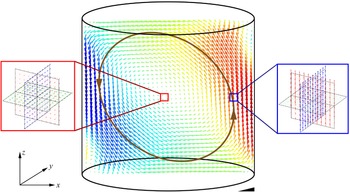
) and Xu et al. (Reference Xu, Zhang and Xia2024). The applied convection cell is a vertical cylinder with a height and inner diameter of 188 mm (unit aspect ratio), as shown in figure 1. To reduce image distortion, a water-filling square jacket is fitted around the 6 mm-thick Plexiglass sidewall. The top plate is made of a sapphire disc with 5 mm thickness to ensure both high thermal conductivity (
 $\lambda _f \approx$
42 W (m K)
 $^{-1}$
) and optical access is from above. There is a cooling chamber for water circulation over the sapphire plate, and the top plate temperature is measured at the disc side by four evenly distributed thermistors. The bottom plate is made of a 30 mm-thick copper disc. The copper plate is coated with a thin layer of Teflon to prevent polymer coagulation. Four embedded thermistors with an even distribution along the peripheral are applied to measure the bottom plate temperature. The thermistors (OMEGA 44031) used to measure the temperatures of the top and bottom plates have an accuracy of 0.01 K and a response time of 1 s. The bulk temperature of the convection cell is measured using a small waterproof thermistor (TE Connectivity NTC, 0.2 mm diameter, 30 ms response time) inserted through the sidewall. The entire convection cell is insulated inside a thermostat to minimise the heat exchange between the convection system and its surroundings, and the thermostat temperature is kept the same as the bulk temperature, i.e.
 $40\,^{\circ }{\textrm{C}}$
. The Cartesian coordinate system has its origin at the measurement position (centre or side),
 $x{-}y$
being the horizontal plane and
 $z$
axis pointing upwards. To avoid the occurrence of flow reversals and the rotation of the circulation plane (Brown, Nikolaenko & Ahlers Reference Brown, Nikolaenko and Ahlers2005; Sun, Xia & Tong Reference Sun, Xia and Tong2005; Xi, Zhou & Xia Reference Xi, Zhou and Xia2006), the cylindrical convection cell was normally tilted slightly to partially lock the orientation of the large-scale circulation. The present cylindrical cell was tilted by around 1
 $^{\circ }$
in the
 $x{-}z$
plane, so that the
 $y$
-axis is now perpendicular to the mean plane of the large-scale circulation.
Sketch of the convection cell and the instantaneous velocity fields in the three orthogonal planes measured by the VGTR-PIV system. The planar mean velocity field across the entire convection cell indicates a single-roll large-scale circulation. The convection cell was tilted in the
 $x{-}z$
plane to partially lock the orientation of the large-scale circulation. The enlarged red and blue regions indicate the measurement positions in the centre and side regions, respectively. The cylindrical convection cell has a diameter and height of 188 mm, with a 5.2 mm
 $\times$
5.2 mm field of view in each orthogonal measurement plane. The black wedge indicates a slight tilt of the convection cell by around 1
 $^{\circ }$
in the
 $x{-}z$
plane.

To spatiotemporally resolve the velocity gradient tensor, we applied a VGTR-PIV system (Xu et al. Reference Xu, Zhang and Xia2024). As shown in figure 1 insets, the planar velocity fields in three orthogonal planes were measured simultaneously, with spatial and temporal resolutions down to the Kolmogorov scales. The velocity gradient tensor was thus fully resolved at the intersection point of the three measurement planes. We used three laser light sheets with wavelengths of 473 nm, 532 nm and 671 nm to illuminate these orthogonal planes, and the thickness of each light sheet is approximately 0.5 mm. Three synchronised CMOS cameras (PCO.edge 5.5M, with 16-bit dynamic range and 6.5 μm
 $\times$
6.5 μm sensor pixel size) were applied to record the image sequences. The cameras were mounted with Nikkor AF 105 mm
 $f$
/2.8 micro lenses, and each lens was equipped with a
 $\pm 10$
nm OD5 bandpass filter with its centre wavelength corresponding to the laser wavelength in each measurement plane. The camera image data was transmitted to disc arrays in real-time using a CameraLink HS connection.
In the VGTR-PIV measurement, the fluid was seeded with Dantec 10 μm diameter hollow glass particles (1.1 g cm
 $^{-3}$
density). The hollow glass spheres were centrifuged to discard particles lighter than water, as light particles attached to the sapphire top plate may block the top optical access. In the present work, the Stokes number varies in a range of
 $St = 3.0 \times 10^{-7} {-} 1.2 \times 10^{-6}$
, indicating that the seeding particles can faithfully follow the fluid motion (Raffel et al. Reference Raffel, Willert, Wereley and Kompenhans2007). The parameters of the calibration functions, which map the three-dimensional laboratory coordinate system onto the camera image plane, were obtained by moving the tip of a steel needle using stepper motors and tracking its displacement in each camera image. Uncertainties caused by thermal plumes and other disturbances can be assessed by tracking the needle tip trajectory in each camera, and the errors were found to be 2.6
 $\unicode{x03BC}$
m in the horizontal plane and 0.9
 $\unicode{x03BC}$
m in the vertical planes (Xu et al. Reference Xu, Zhang and Xia2024). The spatial resolution is
 $6.5$
μm per pixel, corresponding to a 5.2 mm
 $\times$
5.2 mm field of view (800
 $\times$
800 pixels). At each position and polymer concentration, the measurement was conducted at a sampling frequency of 80 Hz for 8.75 hr, i.e.
 $2.52 \times 10^6$
image pairs. The sampling time interval is nearly two orders of magnitude smaller than the Kolmogorov time scales. The sampling period corresponds to
 $1.5 \times 10^{4} {-} 1.9 \times 10^{4}$
times of the free-fall time unit (
 $t_{ff} = \sqrt {H / \alpha g \Delta T}$
), one to two orders of magnitude larger than the statistical time in most numerical simulations. An in-house cross-correlation code implemented on a high-performance parallel computing device was used to process a large number of PIV images (Xu et al. Reference Xu, Zhang and Xia2022, Reference Xu, Zhang and Xia2024). Each frame was divided into interrogation areas of
 $128 \times 128$
pixels with
 $50\,\%$
overlap, leading to a spatial resolution (i.e. the distance between adjacent velocity vectors) of 0.42 mm, which is smaller than the local Kolmogorov length scale of 0.47 mm
 $-$
1.17 mm. Therefore, our VGTR-PIV system spatiotemporally resolves the velocity gradient tensor and the energy dissipation rate. When calculating the in-plane velocity gradient components, five data points centred at the measurement position were used to fit a quadratic function to the velocity profile
 $u_i(x_j)$
, which helps to improve the data quality. To minimise the effect of thermal plumes, we select the normal components
 $\partial u / \partial x$
and
 $\partial w / \partial z$
in the
 $x{-}z$
plane, and
 $\partial v / \partial y$
in the
 $y{-}z$
plane in constructing the full velocity gradient tensor. The relative errors in the velocity gradient tensor are estimated to be 5.2 % for the two shear components
 $\partial u / \partial y$
and
 $\partial v / \partial x$
, and 1.8 % for the remaining seven components. The readers may refer to Xu et al. (Reference Xu, Zhang and Xia2024) for further details of the VGTR-PIV system.
We apply distilled water with polyacrylamide long-chain polymers (PAM; Polysciences Inc. 18522-100; nominal molecular weight
 $18 \times 10^6$
atomic mass units) as the working fluid. As the vendor of the polymer samples did not supply information about the monodispersity, we assume polymers to be polydisperse. The polydispersity may be important in interpreting relevant experimental results (Serafini et al. Reference Serafini, Battista, Gualtieri and Casciola2025). The fully stretched contour length of the polymer molecule is 72
 $\unicode{x03BC}$
m (Zimm Reference Zimm1956), an order of magnitude smaller than the Kolmogorov length scale in the present work. The Weissenberg number, which is the ratio between the stress relaxation time
 $\tau _p$
and the Kolmogorov time scale
 $\tau _{\eta }$
, is estimated to be
 $Wi = \tau _p / \tau _{\eta } = 0.047$
. In turbulent thermal convection, polymers with such a small
 $Wi$
can still have significant effects, which may be attributed to the spatiotemporal inhomogeneity. Xu et al. (Reference Xu, Zhang and Xia2024) found that the time-averaged energy dissipation rate near the wall surfaces can be two orders of magnitude higher than that in the bulk, and the instantaneous dissipation can be more than an order of magnitude higher than its time average, both of which lead to a significant shortening of the Kolmogorov time scale. As a result, the instantaneous Weissenberg number can reach
 $O(1)$
at certain moments and in specific regions, sufficient to stretch polymer molecules. The kinematic viscosity of the polymer solution was calibrated using a glass capillary viscometer immersed in a water bath controlled at the bulk temperature
 $40\,^{\circ }\textrm {C}$
. The kinematic viscosity of the polymer solution can be fitted as
 $\nu (c) / \nu (0) = 1 + 0.0277c$
(Xu et al. Reference Xu, Liu, Li and Xia2025), with the polymer concentration
 $c$
in units of parts per million by weight (p.p.m.). We first prepared the stock solution with a concentration of 1000 p.p.m. by slowly adding the polymer powders to the deionised and degassed water with gentle stirring. Then, the stock solution was stirred for 12 hr and injected into the convection cell. The RBC system was run for 12 hr at each polymer concentration before a measurement was taken to ensure good dispersion and dissolution of polymers throughout the convection cell. The velocity gradient tensor measurements were performed at two representative positions in the convection cell, i.e. centre and side. The side measurement position is located at the middle height and is approximately 12 mm away from the sidewall. In the experiment, the bulk temperature was fixed at
 $40\,^{\circ }\textrm {C}$
(Prandtl number
 $Pr = \nu / \kappa = 4.34$
for water), and the polymer concentration varied from 0 to 20 p.p.m. The Rayleigh number was fixed at
 $Ra = 3 \times 10^9$
, which is achieved by regulating the temperatures of the top and bottom plates to account for the change in the kinetic viscosity.
3. Results and discussions
3.1. Velocity vector and velocity gradient tensor
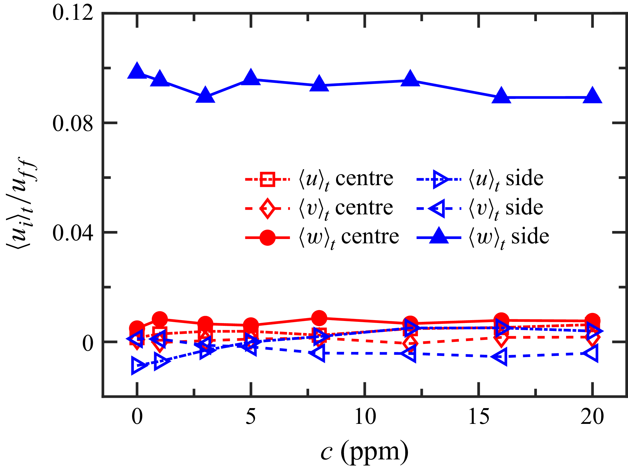
We first study the effects of polymer additives on the properties of the local velocity in the centre and side regions. For the time-averaged velocity components shown in figure 2, the side region remains dominated by an upwelling, while the centre region is still almost static with the addition of polymers. With the slight tilt of the convection cell (around
 $1^{\circ }$
), we find the single-roll large-scale circulation persists for all polymer concentrations (
 $c = 0 {-} 20$
p.p.m.). This indicates that with the explicit symmetry breaking introduced by the tilted convection cell, adding polymers cannot simply restore the axisymmetry, as was observed in Xu et al. (Reference Xu, Liu, Li and Xia2025), which was conducted in a perfectly levelled cell within
 $0.05^{\circ }$
. The degree of symmetry breaking, i.e. the degree of tilting of the convection cell, has a significant influence on the topology of the large-scale flow in polymer RBC.
Time-averaged velocity components in the centre and side regions as a function of polymer concentration. The free-fall velocity
 $u_{ff} = \sqrt {\alpha g H \Delta T}$
is applied to the normalisation.

Figure 3 displays the time series of each velocity component with and without polymer additives. For the horizontal velocity component
 $u$
shown in figure 3(a), the instantaneous value fluctuates around zero, and the fluctuations in the side region are more intense than those in the centre. The addition of polymers significantly suppresses the magnitude of horizontal velocity fluctuations in both measurement positions, as shown in figure 3(b). Besides, adding polymers makes the time series smoother, i.e. the high-frequency velocity fluctuations are inhibited. The same finding applies to the other horizontal velocity component
 $v$
as shown in figure 3(c,d). For the vertical velocity component
 $w$
(see figure 3
e,f), the suppression on the velocity amplitude is less intense compared with the horizontal component, although a filtering of high-frequency velocity fluctuations is also observed.
Time traces of velocity components
 $u$
(a,b),
 $v$
(c,d) and
 $w$
(e,f) in the centre and side regions at polymer concentrations of
 $c = 0$
(a,c,e), and 20 p.p.m. (b,d,f). The dashed lines are the time-averaged values corresponding to each time trace. The origin of the abscissa is chosen arbitrarily.

Figure 4 shows the probability density functions (PDFs) of the horizontal and vertical velocity fluctuations. The PDFs of the horizontal velocity component at different polymer concentrations nearly overlap with each other and follow a Gaussian distribution in the centre region (see figure 4 a,c). For the vertical velocity in the centre region shown in figure 4(e), the tails are slightly above the Gaussian distribution, which is similar to the result in Li et al. (Reference Li, Huang, Ni and Xia2021) and may be attributed to the small passage of the thermal plumes. For the vertical velocity in the side region shown in figure 4(f), the non-Gaussian and asymmetric PDF distribution can be attributed to the strong upwelling of the hot thermal plumes. Although the PDFs at different polymer concentrations basically overlap, there are variations in the magnitude of the velocity fluctuations. Figure 5 shows that the fluctuation magnitude of each velocity component first decreases and then levels off with increasing polymer concentration. The suppression of velocity fluctuations in both centre and side regions exhibits an anisotropy, with vertical fluctuations at the highest polymer concentration exceeding horizontal ones by around 70 %. The anisotropic suppression of velocity fluctuations is qualitatively consistent with the result in Xu et al. (Reference Xu, Liu, Li and Xia2025). At 20 p.p.m. polymer concentration, the ratio between vertical and horizontal velocity fluctuations reaches 3.5 in Xu et al. (Reference Xu, Liu, Li and Xia2025), which exhibits an axisymmetric flow topology in the levelled convection cell, yet it is around 1.7 in the current study, which presents a symmetry breaking in the horizontal direction.
The PDFs of velocity fluctuation components
 $u'$
(a,b),
 $v'$
(c,d) and
 $w'$
(e,f) in the centre (a,c,e), and side (b,d,f) regions. The fluctuating velocity is normalised by its standard deviation. The black curves indicate the Gaussian fittings of the Newtonian case.

Horizontal and vertical components of velocity fluctuations in the absolute (a), and normalised (b) values as a function of polymer concentration.

Figure 6 shows the PDFs of the velocity gradient tensor
 $\partial u_i / \partial x_j$
, which is divided into three normal (
 $i = j$
) and six shear (
 $i \ne j$
) components, in both measurement positions. The three normal components basically overlap and are therefore all included in the PDF statistics, as are the six shear components (Xu et al. Reference Xu, Zhang and Xia2024). The PDFs of the velocity gradient fluctuations at different polymer concentrations substantially overlap. The PDF follows an exponential distribution in the positive and negative tails for each velocity gradient component. With the addition of polymers, the PDF tails become slightly higher in the centre but lower in the side region. Figure 7 indicates that the suppression of the velocity gradient fluctuations is more pronounced in the centre than the side region. In the centre, adding polymers suppresses the normal and shear velocity gradient components approximately equally, with the normal components being slightly lower. In contrast, in the side region, the addition of polymers suppresses the normal velocity gradient components more significantly than the shear components. The anisotropic suppression on the velocity gradient tensor suggests that the strain rate inhibition is stronger than the rotational part.
The PDFs of normal
 $i = j$
(a,c), and shear
 $i \ne j$
(b,d) components of vertical gradient tensor
 $\partial u_i / \partial x_j$
in the centre (a,b), and side (c,d) regions.

Normal (
 $i = j$
), and shear (
 $i \ne j$
) components of the velocity gradient standard deviation
 $\sigma _{\partial u_i / \partial x_j}$
in the absolute (a), and normalised (b) values as a function of polymer concentration.

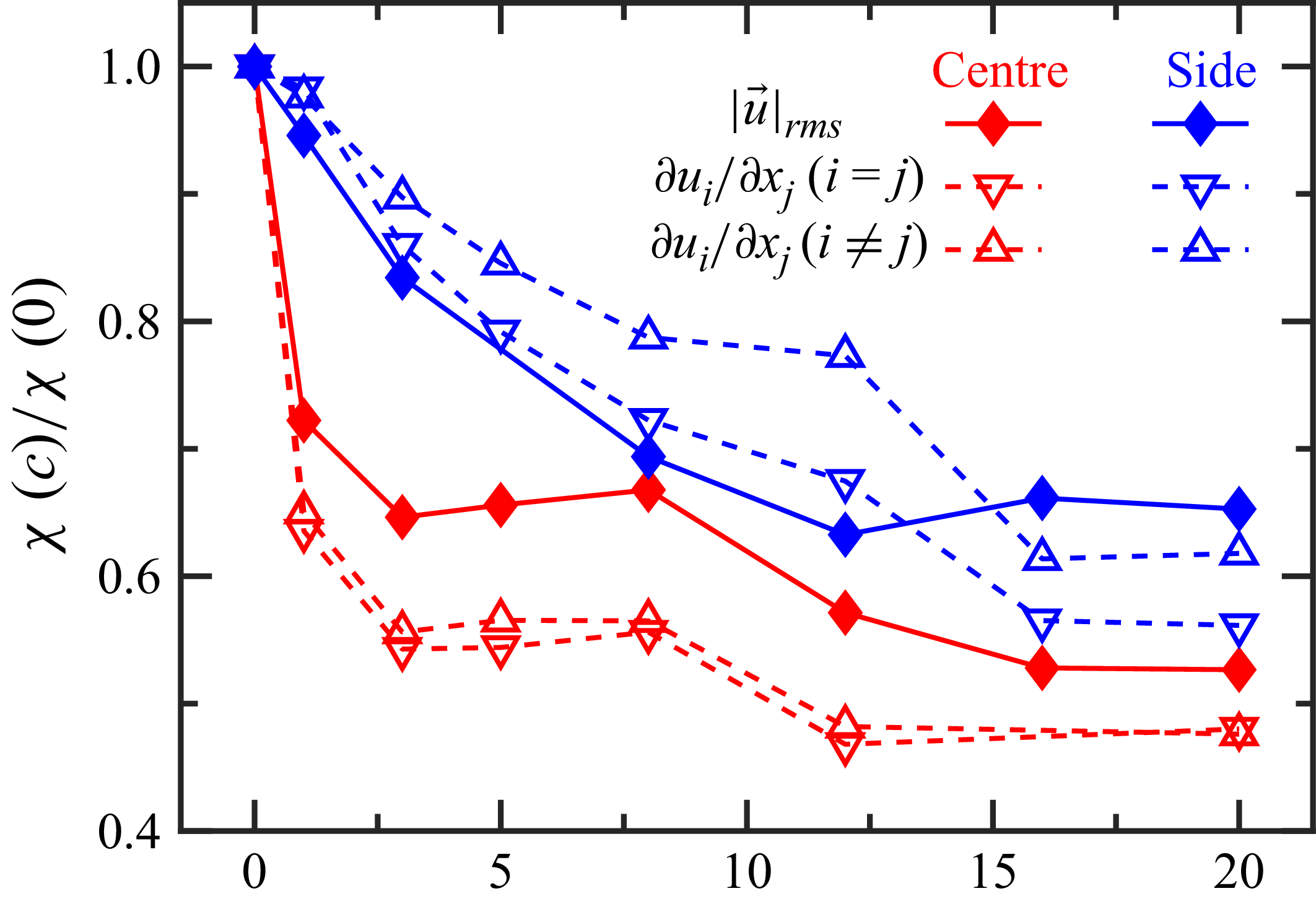
Figure 8 compares the normalised variations of the velocity and the velocity gradient as a function of polymer concentration. The relative ratios of these quantities have lower values in the centre than in the side region. The suppressions in the centre exhibit an abrupt decrease with the introduction of the tiniest amount of polymer, and then level off at a higher polymer concentration. In contrast, the effect of polymers is much more progressive in the side region, as the curves continue to decrease and then saturate at a concentration of 16 p.p.m. A lower value of the normal velocity gradient tensor components compared with the shear components, i.e. stronger inhibition on the strain rate than on the rotational part, can be observed in the two regions.
Variations of velocity and velocity gradient normalised by the Newtonian case as a function of polymer concentration.

The anisotropic properties of the Reynolds stress can be studied based on the full velocity vector. The Reynolds stress tensor
 $\tau _{\textit{ij}} = \langle u_i u_j \rangle _t$
, as a symmetric second-order tensor, characterises the mean momentum transport contributed by turbulence. It should be mentioned that Reynolds stresses are not exactly small-scale features as they may accumulate over scales larger than the dissipative scale. The Reynolds stress tensor is first normalised by twice the turbulence kinetic energy as
 $\tilde {\tau }_{\textit{ij}} = \tau _{\textit{ij}} / \langle u_k u_k \rangle _t$
, and then decomposed into a spherical (isotropic) tensor
 $\tilde {\tau }_{\textit{ij}}^{iso}$
and a traceless (anisotropic) tensor
 $\tilde {\tau }_{\textit{ij}}^{a}$
as
 \begin{equation} \tilde {\tau }_{\textit{ij}}^{iso} = \frac {\delta _{\textit{ij}}}{3}; \quad \tilde {\tau }_{\textit{ij}}^{a} = \frac {\tau _{\textit{ij}}}{\langle u_k u_k \rangle _t} - \frac {\delta _{\textit{ij}}}{3}, \end{equation}
where
 $\delta _{\textit{ij}}$
is the Kronecker delta, and summation over repeated indices is implied. In the isotropic turbulence, the anisotropic tensor
 $\tilde {\tau }_{\textit{ij}}^{a}$
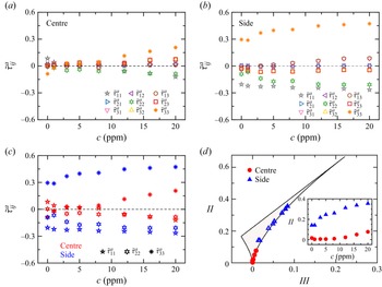
vanishes identically. Figure 9(a,b) plot the dependence of the normalised anisotropic component
 $\tilde {\tau }^{a}_{\textit{ij}}$
on the polymer concentration. While the shear components (
 $i \ne j$
) remain essentially zero within the experimental uncertainty, the addition of polymers significantly influences the normal components (
 $i = j$
) in both measurement regions. Figure 9(c) plots the normal components at different polymer concentrations in the centre and side regions. The normal component is almost zero in the centre at
 $c = 0$
, indicating a local near-isotropy. In the side region at
 $c = 0$
, we observe two negative horizontal components and one positive vertical component, which can be explained by the fact that
 $\tilde {\tau }^{a}_{\textit{ij}}$
is a traceless tensor
 $\tilde {\tau }^{a}_{ii} = 0$
. In each region, all three normal components become larger for the
 $c \gt 0$
cases, with the vertical component being much larger than the two horizontal components (
 $\tilde {\tau }_{zz}^{a} \gt \tilde {\tau }_{xx}^{a} \approx \tilde {\tau }_{yy}^{a}$
). These results are generally consistent with the anisotropic suppression of the velocity fluctuations observed in Xu et al. (Reference Xu, Liu, Li and Xia2025). The anisotropy in turbulent flows is quantified by the anisotropy invariant map in the
 $III{-}II$
coordinate (Lumley Reference Lumley1979), which can be calculated using
 \begin{equation} II = \tilde {\tau }_{\textit{ij}}^{a} \tilde {\tau }_{ji}^{a}, \hspace {5mm} III = \tilde {\tau }_{\textit{ij}}^{a} \tilde {\tau }_{jk}^{a} \tilde {\tau }_{ki}^{a}, \end{equation}
where the invariant
 $II$
measures the degree of anisotropy of the Reynolds stresses, and the invariant
 $III$
characterises the nature of anisotropy. The right-hand curved boundary of the map corresponds to a cigar-shaped axisymmetric expansion, in which one diagonal component of the turbulence kinetic energy is larger than the other two equal components (Choi & Lumley Reference Choi and Lumley2001). Figure 9(d) indicates that the addition of polymers leads to an upper right-hand shift in the anisotropy invariant map, suggesting a ‘cigar-shaped’ expansion in the centre and side regions. The inset in figure 9(d) confirms that the turbulence becomes more anisotropic with the addition of polymers, and the level of anisotropy is stronger in the side region than that in the centre. Although the symmetry-breaking large-scale flow persists in the present study, the momentum transport between the mean flow and turbulence has been modified by the addition of polymers.
(a,b) Normalised anisotropic tensor as a function of polymer concentration in the (a) centre and (b) side regions. (c) Normal components of the normalised anisotropic tensor as a function of polymer concentration. (d) Anisotropy invariant map in the
 $III{-}II$
coordinates. The inset in panel (d) plots the parameter
 $II$
characterising the degree of anisotropy as a function of polymer concentration.

3.2. Energy dissipation rate, enstrophy and streamline flow topology
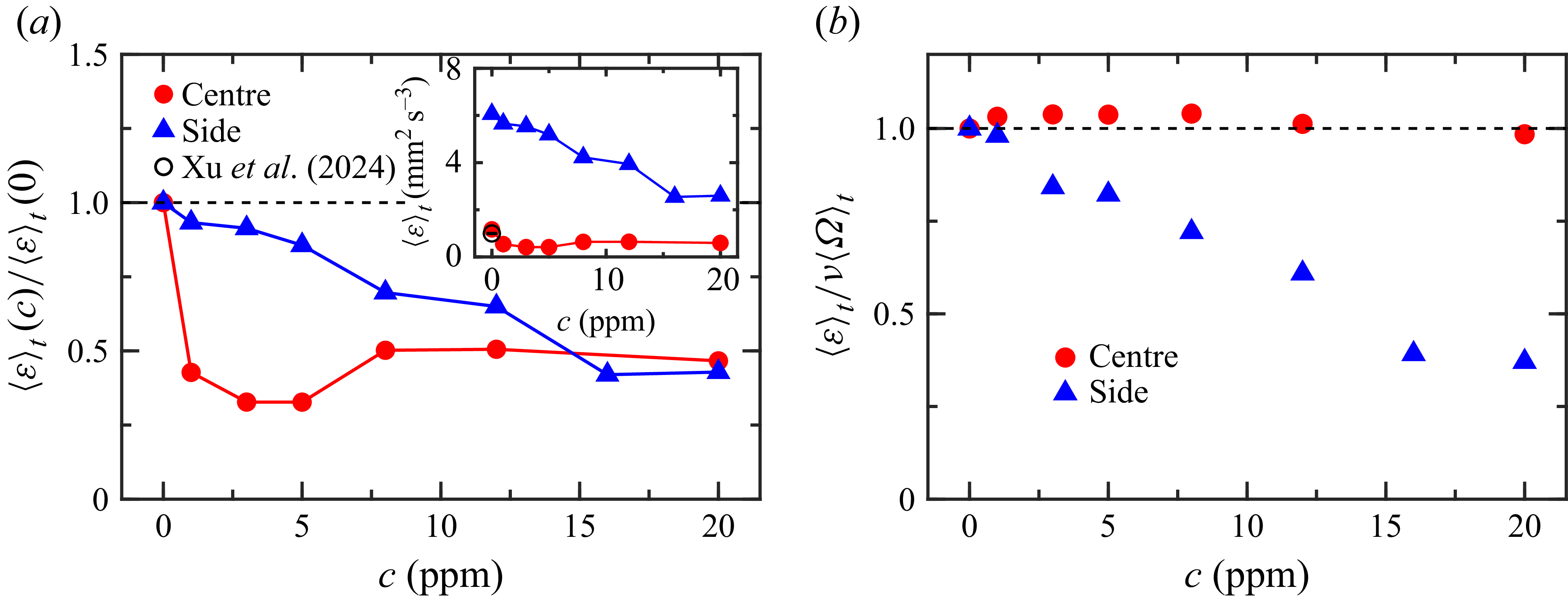
With the spatiotemporally resolved velocity gradient tensor, we can obtain the instantaneous energy dissipation rate defined in (1.2). Figure 10(a) shows the dependence of the time-averaged dissipation rate
 $\langle \varepsilon \rangle _t$
and the polymer concentration in the centre and side regions. In both regions, the dissipation rate first decreases and then levels off with increasing polymer concentration, with a plateau value of around 50 %. In the central region, the decrease of the energy dissipation rate saturates at a low concentration of 1 p.p.m. The abrupt decrease of the energy dissipation at a low concentration in the centre is similar to the trends of the velocity and velocity gradient shown in figure 8. As shown in figure 10(a), the energy dissipation rate measured at the cell centre exhibits a non-monotonic behaviour, it falls very sharply as soon as polymer concentration becomes non-zero and reaches a minimum value at around 5 p.p.m. and then increases again, eventually saturating at higher concentration. The reason for this peculiar non-monotonic behaviour is unknown to us and deserves further investigation. In contrast, the dissipation rate decreases in the side region until a higher concentration of 16 p.p.m. Considering the exact balance between the volume-averaged energy dissipation rate and the global heat transport in (1.3), the decreased dissipation rate in both regions implies a reduction in
 $Nu$
, as observed in the convection cell with smooth conducting plates (Ahlers & Nikolaenko Reference Ahlers and Nikolaenko2010; Wei et al. Reference Wei, Ni and Xia2012). The enstrophy, which is crucial in describing the rotational motion of the turbulent flow, is defined as
 \begin{equation} \varOmega \equiv 2 \omega _{\textit{ij}} \omega _{\textit{ij}}, \end{equation}
where
 $\omega _{\textit{ij}} = (\partial u_i / \partial x_j - \partial u_j / \partial x_i) / 2$
is the rotation rate tensor. For an isotropic turbulence, the energy dissipation rate would balance the enstrophy (Pope Reference Pope2000), i.e.
 \begin{equation} \langle \varepsilon \rangle _t = \nu \langle \varOmega \rangle _t. \end{equation}
The ratio between the energy dissipation rate and the enstrophy, as shown in figure 10(b), quantifies the relative importance between strain rate and rotation. This ratio remains approximately unity in the centre region, consistent with the previous observation that polymers equally suppress the normal and shear velocity gradient components (see figure 7). In the side region, the energy dissipation rate decreases more rapidly than the enstrophy, indicating that the polymer additives have a stronger suppressive effect on strain rate than on rotation. As shown in figure 7, in the side region, the suppression of the normal components in the velocity gradient tensor is stronger than the suppression of the shear components, leading to a stronger suppression of the energy dissipation rate as observed in the inset here.
(a) Time-averaged dissipation rate normalised by its value at
 $c = 0$
as a function of polymer concentration. The open circle in the inset is the reference centre dissipation in Xu et al. (Reference Xu, Zhang and Xia2024). (b) The ratio between the energy dissipation rate and the enstrophy as a function of polymer concentration. This ratio would be unity for an isotropic turbulence.

Based on the time sequence of the velocity gradient tensor, the PDF statistics of the energy dissipation rate and enstrophy can be studied. We emphasise that due to the strong position dependence, a volume averaging may not be very meaningful when measuring an inhomogeneous position, as a linear superposition of multiple (pointwise) exponential distributions will erroneously lead to a spurious stretched exponential distribution (Berberan-Santos, Bodunov & Valeur Reference Berberan-Santos, Bodunov and Valeur2005). This highlights the unique advantages of our pointwise experimental measurements using the VGTR-PIV system. Figure 11 shows the PDFs of the highly intermittent energy dissipation rate and enstrophy in the centre and side regions. In the centre, the PDF curves exhibit a stretched exponential distribution, and the curve shapes are independent of the polymer concentration. The higher tail shown in figure 11(b) compared with the tail shown in figure 11(a) suggests that extreme events with high enstrophy are more probable than the extreme dissipative rate, similar to the observations in Yeung, Zhai & Sreenivasan (Reference Yeung, Zhai and Sreenivasan2015). In the side region, the PDF tail decreases with increasing polymer concentration, indicating that adding polymers can effectively suppress extreme dissipative and rotational events. The PDF of the energy dissipation rate or the enstrophy exhibits a stretched exponential distribution at low concentration and gradually changes to an exponential one as the concentration increases. The exponential distribution may be attributed to the stabilising effect of polymer additives on the viscous boundary layer (Cheng et al. Reference Cheng, Zhang, Cai, Li and Li2017) and the conditional statistics inside and outside the viscous boundary layer in Xu et al. (Reference Xu, Zhang and Xia2024).
The PDFs of the energy dissipation rate (a,c), and enstrophy (b,d) in the centre (a,b), and side (c,d) regions. The black solid curves in each panel indicate the stretched exponential fittings at
 $c = 0$
. The black straight lines in panels (c) and (d) indicate exponential fittings at the polymer concentration of 20 p.p.m.

Next, we investigate the effects of polymers on the simultaneous occurrence of dissipative and rotational events. The probability ratio which characterises the interdependence of the energy dissipation rate
 $\varepsilon$
and the enstrophy
 $\varOmega$
is defined as
 \begin{equation} {\mathcal{P}} = \frac {P(\varepsilon , \varOmega )}{P(\varepsilon ) P(\varOmega )}, \end{equation}
where
 $P(\varepsilon , \varOmega )$
is the joint probability. The probability ratio is unity (
 ${\mathcal{P}} = 1$
) when these two quantities are statistically independent. A probability ratio greater than one indicates that the two quantities are likely to co-occur at the given values, and a higher value in
 $\mathcal{P}$
indicates a higher probability of co-occurrence. Figure 12 shows the effect of polymer additives on the probability ratio between energy dissipation rate and enstrophy. In the centre, extreme events with high dissipation and enstrophy are more likely to co-occur as the polymer concentration increases. In the side region, the extreme events with a high probability ratio are over the dotted line. In addition to the extreme events, the higher probability ratio in the lower left-hand region indicates that low dissipation and low enstrophy are more likely to co-occur in the side region. Since the turbulence becomes less intense (see figure 5), the interdependence of dissipation and enstrophy should be smaller; therefore, the change in the probability ratio distribution should be uniquely attributed to adding polymers.
Probability ratio of enstrophy and energy dissipation rate at polymer concentrations of
 $c = 0$
(a,d), 5 p.p.m. (b,e) and 20 p.p.m. (c,f) in the centre (a–c), and side (d–f) regions. The dotted line in each panel corresponds to a slope of one with
 $\varepsilon / \langle \varepsilon \rangle _t = \varOmega / \langle \varOmega \rangle _t$
.

The instantaneous velocity gradient tensor (
 $\boldsymbol{A}$
,
 $a_{\textit{ij}} = \partial u_i / \partial x_j$
) can be decomposed into different terms to analyse their contributions separately. Based on the tensor symmetry, the velocity gradient tensor can be decomposed into strain rate and vorticity contributions
 \begin{equation} \boldsymbol{A}^2 = \boldsymbol{S}^2 + \boldsymbol{W}^2, \end{equation}
where
 $s_{\textit{ij}} = (\partial u_i / \partial x_j + \partial u_j / \partial x_i) / 2$
in the strain rate tensor
 $\boldsymbol{S}$
and
 $\omega _{\textit{ij}} = (\partial u_i / \partial x_j - \partial u_j / \partial x_i) / 2$
in the rotation rate tensor
 $\boldsymbol{W}$
. However, this decomposition cannot effectively distinguish the normal strain and the rigid-body rotation, and the shear exists in both the strain rate and the vorticity (Kolář Reference Kolář2007). To address this issue, the spatiotemporally resolved velocity gradient tensor (
 $\boldsymbol{A}$
) can be triply decomposed into normal strain rate (
 $\boldsymbol{N}$
), pure shearing (
 $\boldsymbol{H}$
) and rigid-body rotation rate (
 $\boldsymbol{R}$
) (Tian et al. Reference Tian, Gao, Dong and Liu2018; Das & Girimaji Reference Das and Girimaji2020). The normal strain-rate tensor represents the compression/extension of the fluid element, the pure shearing measures the shearing of the fluid element by the transverse velocity gradients and the rigid-body rotation rate corresponds to the pure rotation of the fluid element. The magnitude of the velocity gradient tensor, in its Frobenius norm, can be decomposed as
 \begin{equation} \boldsymbol{A}^2 = \boldsymbol{N}^2 + \boldsymbol{H}^2 + \boldsymbol{R}^2 + 2 \boldsymbol{R} \boldsymbol{H}, \end{equation}
where the additional term
 $\boldsymbol{R} \boldsymbol{H} = R_{\textit{ij}} H_{\textit{ij}}$
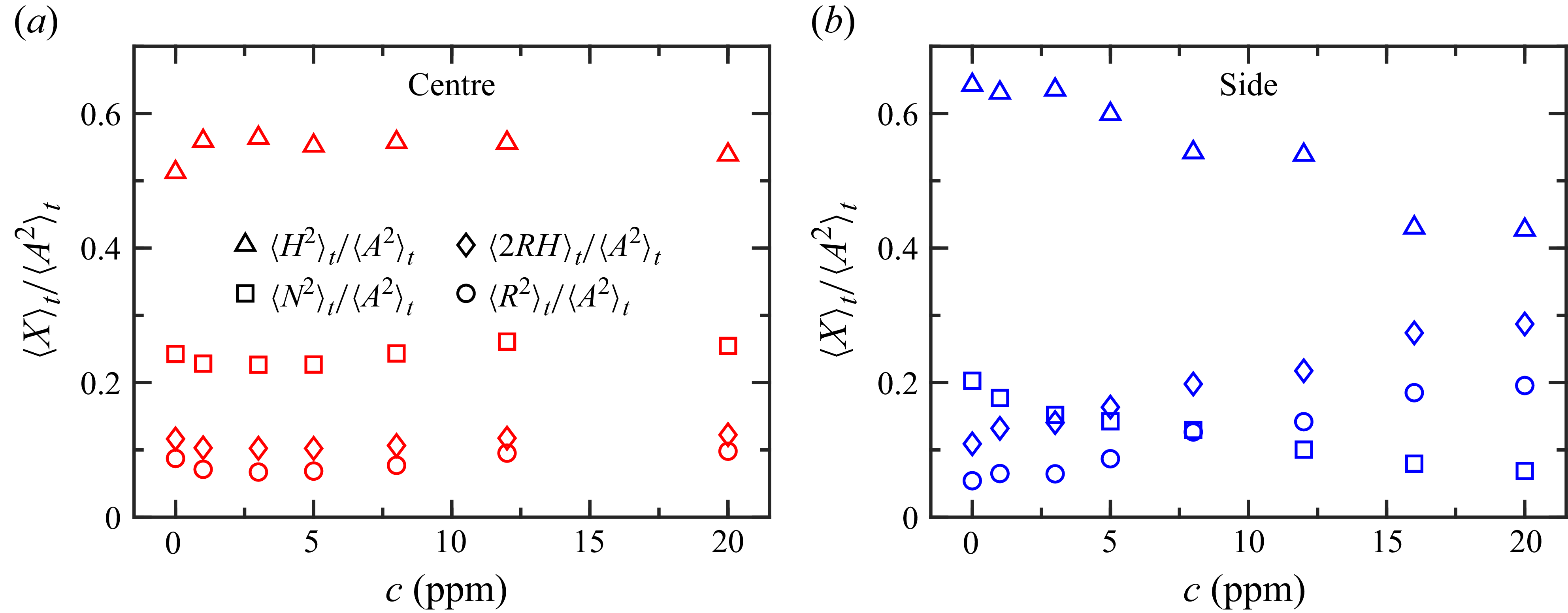
is the shear-rotation correlation. Figure 13 separates the mean contributions of the four terms to the velocity gradient tensor. In the centre region, adding polymers does not change the relative contributions of the four terms to the velocity gradient tensor. In contrast, in the side region, there is an increase in the contributions of rigid-body rotation and shear-rotation correlation. We have observed that the suppression of the strain rate (
 $\boldsymbol{S}$
) is stronger than that of rotation (
 $\boldsymbol{W}$
) with the addition of polymers (see figure 10). Based on the triple decomposition, the strain rate tensor can be written as
 \begin{equation} \boldsymbol{S}^2 = \boldsymbol{N}^2 + \boldsymbol{H}^2 / 2, \end{equation}
and the rotation tensor as
 \begin{equation} \boldsymbol{W}^2 = \boldsymbol{R}^2 + 2 \boldsymbol{R} \boldsymbol{H} + \boldsymbol{H}^2 / 2. \end{equation}
Therefore, the difference in the dissipation rate and the enstrophy comes from the increase of both pure rotation and shear-rotation correlation, along with the decrease in the normal strain rate, as shown in figure 13(b).
Contributions to the magnitude of velocity gradient tensor (
 $\boldsymbol{A}^2$
) by normal strain rate (
 $\boldsymbol{N}^2$
), rigid body rotation (
 $\boldsymbol{R}^2$
), pure shear (
 $\boldsymbol{H}^2$
) and shear-rotation correlation (
 $2 \boldsymbol{R} \boldsymbol{H}$
) as a function of polymer concentration in the centre (a), and side (b) regions.

The local streamline topology identifies key universal features of the local streamline structure and turbulence dynamics, which can be studied using the matrix invariants of the measured velocity gradient tensor (Chong, Perry & Cantwell Reference Chong, Perry and Cantwell1990). The characteristic equation of the velocity gradient tensor is written as
 $\lambda ^3 + P \lambda ^2 + Q \lambda + R = 0$
, with invariants
 $P = -s_{ii} = 0$
for an incompressible flow,
 $Q = (-s_{\textit{ij}} s_{\textit{ij}} + r_{\textit{ij}} r_{\textit{ij}}) / 2$
representing the competition between strain rate and rotation and
 $R = -(s_{\textit{ij}} s_{jk} s_{ki} + r_{\textit{ij}} r_{jk} r_{ki}) / 3$
indicating whether the local flow is stable. The relative uncertainties of these invariants
 $Q$
and
 $R$
are estimated to be 10.1 % and 15.4 %, respectively. Figure 14 shows the joint PDF of the
 $Q$
and
 $R$
invariants of the velocity gradient tensor. At
 $c = 0$
, the joint PDF of
 $Q$
and
 $R$
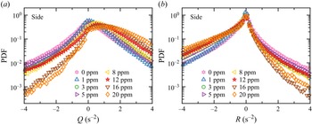
exhibits a teardrop shape, a universal feature of shear flows and isotropic turbulence (Wallace Reference Wallace2009). In the centre region, the joint PDF changes from a teardrop shape to an olive shape with increasing polymer concentration. In the side region, the joint PDF also deviates from the teardrop shape, with a reduction in size in the right-hand tail. As shown in figure 15, the PDF distribution has an increase in positive
 $Q$
and negative
 $R$
with increasing polymer concentration, i.e. the strain rate is suppressed more strongly than the rotation, and the local flow topology becomes more stable. The stronger suppression on the strain rate than the rotation shown in figure 15(a) is consistent with the result shown in figure 10. The stabilising effect based on the local streamline topology shown in figure 15(b) is consistent with the thermal boundary layer stabilisation observed in Cheng et al. (Reference Cheng, Zhang, Cai, Li and Li2017).
Joint PDF of the
 $Q$
and
 $R$
invariants of the velocity gradient tensor at polymer concentrations of
 $c = 0$
(a,d), 5 p.p.m. (b,e) and 20 p.p.m. (c,f) in the centre (a–c), and side (d–f) regions. The white curves
 $27 R^2 + 4 Q^3 = 0$
are the locus of zero values of the cubic discriminant of the velocity gradient tensor, i.e. Vieillefosse lines.

The PDFs of invariants
 $Q$
(a), and
 $R$
(b) of the velocity gradient tensor in the side region.

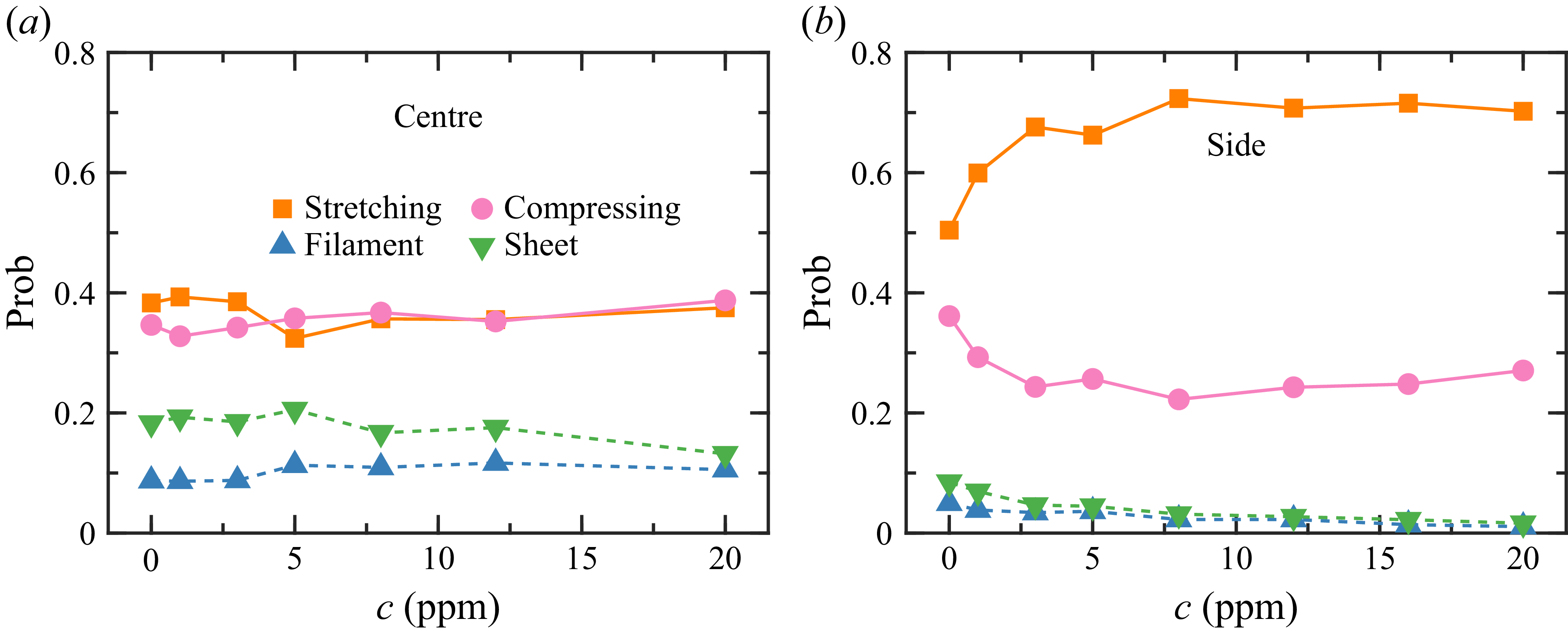
Relative weight of four streamline topologies including stable focus-stretching, unstable focus-compressing, filament and sheet as a function of polymer concentration in the centre (a), and side (b) regions.

The relative weights of different streamline topologies can be obtained by identifying each topology and integrating the joint PDF in the
 $Q{-}R$
plane. In figure 14, the white curves, i.e. the Vieillefosse lines, distinguish the cases with complex eigenvalues featuring rotation from those with only three real eigenvalues (Vieillefosse Reference Vieillefosse1984). Based on the Vieillefosse lines and the sign of
 $R$
, four non-degenerate streamline topologies can be distinguished, including vortex stretching, vortex compressing, filament and sheet (Chacin & Cantwell Reference Chacin and Cantwell2000), with their probabilities calculated and shown in figure 16. In the centre region, the probabilities of these four topologies essentially do not change with the addition of polymers. In the side region, the likelihood of the vortex stretching topology becomes higher, while the other three topologies are relatively inhibited. The increased likelihood in the vortex stretching topology is consistent with the occurrence of the ‘cigar-shaped’ expansion observed earlier in figure 9(d).
3.3. Helicity density
The helicity density, defined as
 $H = \boldsymbol u \boldsymbol{\cdot }\boldsymbol \omega$
, is a topological interpretation of the linkage and knottedness of vortex lines, where
 $\boldsymbol u$
is the velocity and
 $\boldsymbol \omega$
is the vorticity (Moffatt & Tsinober Reference Moffatt and Tsinober1992). As an invariant of the Euler equations, the helicity density plays an essential role in the evolution of turbulent flows. Figure 17 shows PDFs of helicity density in the centre and side regions. The magnitude of the instantaneous helicity density in the side region is more significant than that in the centre. In the centre region, the PDF tail decreases with a minute amount of polymer (1 p.p.m.), and the distributions overlap at different polymer concentrations. In contrast, in the side region, the PDF tail gradually decreases with increasing polymer concentration. The abrupt change in the centre may primarily be attributed to the rapid decrease in the flow intensity, as also observed in the rapid change of relative ratio in figure 8. Correspondingly, in the side region, the gradual decrease in the PDF of the helicity density is consistent with the progressive decrease in the relative ratio. For each region, the normalised PDFs of helicity density at different polymer concentrations essentially overlap. The normalised helicity density in the centre exhibits a stretched tail, similar to the simulation in the forced isotropic turbulence (Choi, Kim & Lee Reference Choi, Kim and Lee2009). In the side region, the helicity density PDF follows an exponential distribution, indicating that it is less intermittent than the central region.
The PDFs of the helicity density in dimensional (a,c), and normalised (b,d) values in the centre (a,b), and side (c,d) regions.

The relative helicity density can be introduced to study only the directional properties, since the helicity density contains information about both magnitude and direction of the velocity and vorticity. The relative helicity density, which is defined as
 \begin{equation} h = {\textrm {cos}}(\boldsymbol u, \boldsymbol \omega ) = \frac {\boldsymbol u \boldsymbol{\cdot }\boldsymbol \omega }{\left | \boldsymbol u \right | \left | \boldsymbol \omega \right |}, \end{equation}
is independent of the magnitudes but only depends on the directional interaction between velocity and vorticity vectors. The relative helicity density is expected to depress the nonlinear energy-transfer process, which is easily understood considering the trigonometric identity
 \begin{equation} \frac {(\boldsymbol u \times \boldsymbol \omega )^2}{\left | \boldsymbol u \right |^2 \left | \boldsymbol \omega \right |^2} + \frac {(\boldsymbol u \boldsymbol{\cdot }\boldsymbol \omega )^2}{\left | \boldsymbol u \right |^2 \left | \boldsymbol \omega \right |^2} = 1, \end{equation}
and the term
 $\boldsymbol \omega \times \boldsymbol u$
in the momentum equation
 \begin{equation} \frac {\partial \boldsymbol u}{\partial t} + \boldsymbol \omega \times \boldsymbol u = - \frac {1}{\rho }\boldsymbol{\nabla }p - \boldsymbol{\nabla }\left ( \frac {\boldsymbol u \boldsymbol{\cdot }\boldsymbol u}{2} \right ) + \nu {{\nabla} ^2}\boldsymbol u + \alpha g \delta T \delta _{i3}, \end{equation}
where
 $p$
is pressure and
 $\delta _{i3}$
is the Kronecker delta. When the velocity and vorticity are parallel, i.e.
 $h$
dominates and
 $\boldsymbol u \times \boldsymbol \omega = 0$
in (3.11), the nonlinear energy transfer in (3.12) is prohibited, and the dissipation becomes lower (Hussain Reference Hussain1986). As shown in figure 18, the PDFs of the relative helicity density are essentially uniform in the centre region, which is similar to the result observed in isotropic turbulence (Rogers & Moin Reference Rogers and Moin1987). In the side region, the velocity tends to be perpendicular to the local vorticity, and this perpendicularity is enhanced with increasing polymer concentration, resulting in an enhancement of the nonlinear energy transfer down to the small scales. These findings are quantified in the inset of figure 18(a), where smaller variance corresponds to a higher probability of orthogonality.
The PDFs of the relative helicity density
 $h = {\textrm {cos}}(\boldsymbol u, \boldsymbol \omega )$
in the centre (a), and side (b) regions. The inset in panel (a) plots the variance of relative helicity density
 $\langle h^2 \rangle _t$
as a function of polymer concentration, where the dashed line
 $\langle h^2 \rangle _t = 1/3$
corresponds to the value of a uniform distribution.

The PDFs of the relative helicity density conditioned on the energy dissipation rate at polymer concentrations of
 $c = 0$
(a,c), and 20 p.p.m. (b,d) in the centre (a,b), and side (c,d) regions.

The helicity density can be related to the magnitude of the energy dissipation rate. Moffatt (Reference Moffatt1985) speculated that high relative helicity density is associated with low energy dissipation rate, and vice versa. The regions between the high helicity density areas will likely be vortex sheets exhibiting a high viscous dissipation rate (Moffatt & Tsinober Reference Moffatt and Tsinober1992). We study the PDFs of relative helicity density conditioned on the local dissipation, as shown in figure 19, with darker colours indicating more dissipative results. In the centre region, there is no significant correlation between the relative helicity density and the dissipation rate. This suggests that, due to the presence of the buoyancy force, the turbulent flow in the centre region differs from the homogeneous and isotropic turbulence. In the side region at
 $c = 0$
, low values of the relative helicity density are associated with high dissipation values, as shown in figure 19(c). Similar features are observed in the conditional PDF with polymer additives (20 p.p.m.) in figure 19(d). Our results support Moffatt’s argument (Moffatt Reference Moffatt1985) that the nonlinear energy transfer, which naturally involves the energy dissipation, is enhanced when the velocity and vorticity are perpendicular.
3.4. Acceleration statistics
The local acceleration can be spatiotemporally resolved using our VGTR-PIV system in the centre and side regions. Using the data measured in the Eulerian frame, the acceleration vector can be calculated (in components) as
 \begin{equation} a_i = \frac {{\textrm{d}} u_i}{{\textrm{d}} t} = \frac {\partial u_i}{\partial t} + u_j \frac {\partial u_i}{\partial x_j}. \end{equation}
Since the acceleration is usually measured using particle tracking velocimetry (PTV) in the Lagrangian frame, we demonstrate the effectiveness of our Eulerian-frame-based method. Figure 20 shows the overlapped PDFs of the three centre acceleration components, confirming the local isotropy of the velocity field in the centre (Sun, Zhou & Xia Reference Sun, Zhou and Xia2006; Zhou, Sun & Xia Reference Zhou, Sun and Xia2008). Our results are consistent with the data in Li et al. (Reference Li, Huang, Ni and Xia2021) measured using PTV at a similar
 $Ra$
.
The PDFs of the normalised acceleration components in the centre of the Newtonian fluid. The open square is the reference PTV-measured vertical acceleration in the Lagrangian frame in Li et al. (Reference Li, Huang, Ni and Xia2021).

Figure 21 plots time traces of the vertical acceleration component without and with polymers. Adding polymers reduces the magnitude of instantaneous vertical acceleration in both centre and side regions. In the side region, the Newtonian case plotted in figure 21(c) presents both positive and negative peaks, while adding polymers causes a negative skew in the vertical acceleration as shown in figure 21(d). The negative skew indicates the deceleration effect caused by the polymer, which is apparent in the PDFs of the normalised vertical acceleration component shown in figure 22. In the centre region, the PDFs at different polymer concentrations essentially overlap. The PDF exhibits a higher peak near zero as the polymer concentration increases, indicating a higher probability of horizontal accelerations. In the side region, the positive tail decreases, indicating that the fluid is more likely to slow down with increasing polymer concentration. Figure 23 shows the directional characteristics of the acceleration vector. As polymer is added, the acceleration vector tends to be in the horizontal direction in the centre. In the side region, the acceleration vector prefers to align with the positive vertical axis. This preferential arrangement is consistent with the increasing deceleration effect with increasing polymer concentration. The phenomenon may be attributed to the slowdown of thermal plumes in the side region with the addition of polymers (Cheng et al. Reference Cheng, Zhang, Cai, Li and Li2017). These findings have potential implications for regulating the transport of substances carried by the large-scale flow in the RBC system.
Time traces of the vertical acceleration component in the centre (a,b) and side (c,d) regions at polymer concentrations of
 $c = 0$
(a,c), and 20 p.p.m. (b,d). The origin of the abscissa is chosen arbitrarily.

The PDFs of acceleration components
 $a_x$
(a,b),
 $a_y$
(c,d) and
 $a_z$
(e,f) in the centre (a,c,e), and side (b,d,f) regions. The acceleration component is normalised by its standard deviation.

The PDFs of the alignment between the acceleration vector and the vertical coordinate axis in the centre (a), and side (b) regions.

In buoyancy-driven turbulence, an interesting question is whether buoyancy dominantly drives the acceleration, which can be addressed by studying the Lagrangian dynamics. With the addition of polymers, the momentum equation with the Oberbeck–Boussinesq approximation is written as
 \begin{equation} \boldsymbol a = \frac {\partial \boldsymbol u}{\partial t} + \boldsymbol u \boldsymbol{\cdot }\boldsymbol{\nabla }\boldsymbol u = - \frac {1}{\rho } \boldsymbol{\nabla }p + \nu \boldsymbol{\nabla} ^2 \boldsymbol u + \alpha g \delta T \boldsymbol e_z + \nu _p \boldsymbol{\nabla }\boldsymbol{\cdot }\boldsymbol{\mathcal{T}}, \end{equation}
where
 $\nu _p$
is the kinematic viscosity of polymers,
 $\boldsymbol{\mathcal{T}}$
in the last term is the stress tensor due to the entropic restoring force of polymer additives. Figure 24 compares variances of the vertical acceleration component
 $a_z$
and the local buoyancy term
 $\alpha g \delta T$
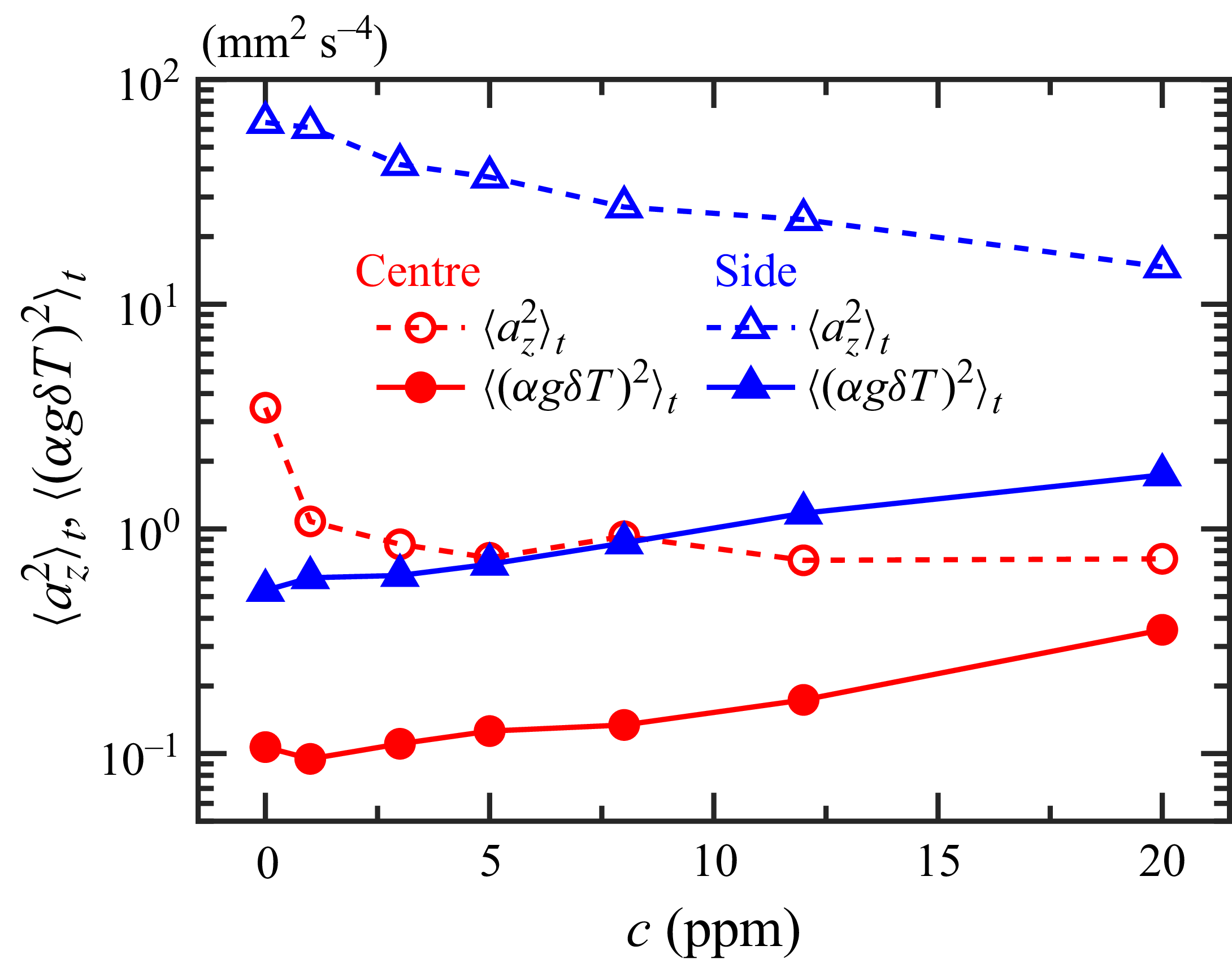
. For the Newtonian fluid, the variance of the buoyancy term is nearly two orders of magnitude smaller than that of the directly measured acceleration (
 $\langle (\alpha g \delta T)^2 \rangle _t \ll \langle a_z^2 \rangle _t$
) in both regions. Therefore, the local acceleration of the Newtonian case is not directly driven by the local buoyancy, which is consistent with previous results (Pandey & Verma Reference Pandey and Verma2016; Li et al. Reference Li, Huang, Ni and Xia2021). With an increased plume coherency, polymer additives increase the variance of the buoyancy term, making it closer to the acceleration variance. However, the acceleration variance is still twice as large as the buoyancy contribution in the centre and nearly one order of magnitude larger than the buoyancy contribution in the side region, even at the highest polymer concentration. Therefore, with polymers, although the buoyancy plays a more important role with increasing polymer concentration, the acceleration is still not directly driven by the local buoyancy.
Comparison between the vertical acceleration variance
 $\langle a_z^2 \rangle _t$
and the variance of the local buoyancy term
 $\langle ( \alpha g \delta T )^2\rangle _t$
as a function of polymer concentration.

4. Conclusions
We have experimentally studied the local velocity gradient tensor and the dissipative properties in a cylindrical RBC cell, with the addition of a tiny amount of long-chain polymer. The convection cell was slightly tilted during the experiment. As a result, the single-roll large-scale circulation persists even in the presence of polymers. High-resolution measurements of the pointwise velocity, velocity gradient tensor and temperature were conducted simultaneously in the centre and side regions, respectively, at Rayleigh number
 $Ra = 3 \times 10^9$
, Prandtl number
 $Pr = 4.34$
for the Newtonian fluid, and polymer concentration up to 20 p.p.m. Adding polymers significantly weakens both velocity and velocity gradient fluctuations, and the stabilising effect is anisotropic in that fluctuations in the horizontal velocity are in general being suppressed more than they are in the vertical one. The increased anisotropy is quantified by the invariants of the Reynolds stress tensor. The mean energy dissipation rate in both regions decreases and then levels off with increasing polymer concentration. In the side region, the energy dissipation rate decreases more rapidly than the enstrophy, indicating that polymer additives have a stronger stabilising effect on strain rate than on vorticity (rotation). The anisotropic suppression is reflected in the co-occurrence of dissipative and rotational events, the velocity gradient triple decomposition and the local streamline topology. The perpendicular alignment between velocity and vorticity, which characterises a nonlinear energy cascade down to small scales, becomes more pronounced with increasing polymer concentration. For the local acceleration, the addition of polymers leads to a deceleration effect in the side region, and the local buoyancy drives the flow more significantly. In summary, our spatiotemporally resolved velocity gradient tensor study shows an increased anisotropy level, indicating that polymers can significantly modify local flow field properties, thus enriching our understanding of viscoelastic thermal convection.
Funding
We gratefully acknowledge the support of this work by the National Natural Science Foundation of China (NSFC) (nos. 12572251, 12202174, 12232010, 12595300, 12595302) and the Centre for Computational Science and Engineering of Southern University of Science and Technology.
Declaration of interests
The authors report no conflict of interest.