

1. Introduction
This article looks at the role of socio-economic status as a determinant of fertility and social mobility in pre-industrial England. We do this using demographic data compiled by the Cambridge Group and documented by Wrigley et al. (Reference Wrigley, Davies, Oeppen and Schofield1997). The data cover 26 parishes scattered across England in a way that was intended to make them representative of the entire country. In addition to information on the number of children being born to each family, the data also sometimes record the occupations of parents and their offspring, which we use to describe the socio-economic status of individuals, as well as intergenerational social mobility within families.
We find that the Cambridge data support the findings of Clark and Hamilton (Reference Clark and Hamilton2006) and Clark (Reference Clark2007), who look at the relationship between wealth and fertility as implied by information recorded in wills, namely that individuals from wealthier social groups were more successful in terms of reproduction. We also investigate the mechanisms by which the poorer groups in society limited their fertility, finding that this was achieved primarily by women delaying marriage.
Clark suggests that a fertility gap between the rich and the poor could have had important implications for the spread of ‘middle-class values’ through English society prior to the Industrial Revolution via downward social mobility. He describes the middle class as being ‘patient, less violent, harder working, more literate, more thoughtful’ (Clark Reference Clark2007, pp. 183–4). Clearly, due to the nature of most of these terms we cannot test directly if ‘middle-class values’ really did come to dominate in society. Nevertheless, he states that these values spread by virtue of the fact that the structure of society was rather stable, which meant there was not enough room at the top for the children of the rich, who thereby were forced to move into other classes.
This twin prediction, that the rich had more children and that society was socially static, is indeed a testable hypothesis. Yet, while Clark's postulates have been subject to a hefty debate, particularly in the present journal (Clark Reference Clark2008; Grantham Reference Grantham2008; McCloskey Reference McCloskey2008; Persson Reference Persson2008; Voth Reference Voth2008), very few attempts have been made to visit the relevant evidence in order to confirm or refute his propositions. Clark himself seems rather agnostic on the actual mechanisms spreading these values. If this was indeed happening then it raises a number of crucial questions: was the spread of middle-class values due to a Lamarckian process of cultural transmission or one of genetic survival, which seems to be gaining ground as an explanation within Unified Growth Theory (Galor and Moav Reference Galor and Moav2002; Galor Reference Galor, Aghion and Durlauf2005)? We also seek to shed light on this question.
2. The data
2.1. Description of the data
Building on statistics collected from Anglican parish registers over the past forty years by the Cambridge Group, the family reconstitution data, documented by Wrigley et al. (Reference Wrigley, Davies, Oeppen and Schofield1997), provide an extraordinary opportunity for testing the hypothesis of the survival of the richest, as well as investigating social mobility in England as a whole. The data cover an extensive period, 1541–1871, although the exact size of the samples we make use of below depends on the variables we look at.
The data are based on so-called family reconstitution forms (FRFs), each of which builds on a marriage (with a unique FRF number). Table 1 offers an example of a family reconstitution form. While the handwritten text may be difficult to read, a complete marriage form (not all information is always reported) includes the dates of birth and death (or baptism/burial) of the spouses, their marriage date, their number of offspring and the offspring's birth and death dates and, finally, the spouses’ occupations at marriage and at death. Importantly, if the couple's offspring themselves went on to marry (as is the case for children 1, 3 and 9 in Table 1 below), then the family reconstitution form will link us to the marriage, and hence a family reconstitution form for the offspring. That way we are able to draw a connection between the occupational status of the parents and their offspring.
Family reconstitution form

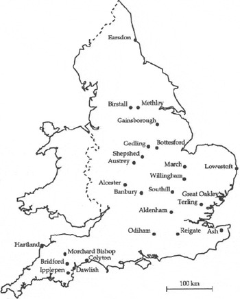
The Cambridge data offer three main advantages compared to the data on which Clark et al. draw their conclusions. Firstly, they include a wide range of the population, while Clark's data tend to cover just the wealthier, i.e. those who left a will. Secondly, while Clark's data cover only a fraction of England, mainly East Anglia but also London, Bristol and Darlington, the Cambridge data cover a much larger geographical area, comprising 26 parishes scattered across England in a way that makes them representative of the entire country.Footnote 1
Last but not least, the Cambridge data offer much richer demographic information than the Clark data, concerning both the reproductive success of families and social mobility across generations within families. For example, ‘surviving offspring’ in the Clark–Hamilton study are the number of children included in the will (Clark and Hamilton Reference Clark and Hamilton2006). This is regardless of the offspring's age at the time of death of the testator, which of course is not specified in the will (indeed, an heir may be just one or two years old). In addition to that, there is a risk that children were excluded from the will. The Cambridge data, on the other hand, allow a calculation, not only of the number of children born to a family (as registered in the church books), but also the number of these children who survived their childhood, i.e. remained alive at least until age 15.
There are also several weaknesses in the Cambridge data set compared to that of Clark and co-authors. A major problem for us with the Cambridge records is that they include no direct information on the wealth of families, whereas Clark and Hamilton (Reference Clark and Hamilton2006), Clark (Reference Clark2007), Clark and Cummins (Reference Clark and Cummins2009, Reference Clark and Cummins2010) all use wealth as the predictor of net fertility. However, the fact that the Cambridge data record parental occupation enables us to make a comparison of reproductive success based on occupational status. Moreover, since the will data occasionally report the occupation of heirs, we can make some headway beyond the Clark–Hamilton study by analysing social mobility across generations within families.
Another drawback of the Cambridge data set is the data missing due to migration out of the parishes scrutinized by the Cambridge Group (Souden Reference Souden1984). We will bias our estimates of fertility downwards if we do not take account of the fact that fathers might move out of the parish during their lifetime, thus leaving us with an incomplete record of their offspring. We take account of this by only looking at fathers for whom we know the death dates, thus making it very likely that they stayed in the same parish after getting married.
Finally, it is worth mentioning that, while the Cambridge data are mostly rural in character, the data of Clark et al. also include men from urban areas. This means that our data become less representative as England urbanized – a point we will return to later. However, our data also come from larger market towns such as Gainsborough and Banbury, and, in general, the reconstitution parishes are larger than average, with an average of 2,187 inhabitants as opposed to 860 inhabitants for all parishes in England in 1801 (Wrigley et al. Reference Wrigley, Davies, Oeppen and Schofield1997).
2.2. Availability and classification of occupations
Since males at the time were far more often in the labour market than females, the occupations of women are very often missing in the data, so we focus exclusively on the occupational link in the data between fathers and sons. When available, we use the occupation at marriage for both sons and fathers. Often, we only have occupation at death available and we use this information instead. A possible concern is that occupations are only recorded for a biased subsample of the population. In an attempt to check this, we have compared fertility in each year for the whole sample with that for our subsample, and the numbers are virtually identical.
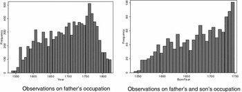
In the period up to 1825Footnote 2 the sample includes observations for a total of 89,887 fathers. Occupation is known for 15,159 of these, but since we also require that fathers have their death dates reported (so as to avoid the possibility that they left the parish before completing their reproductive activities), this leaves us with 9,925 fathers. Among these, 2,778 have reported occupation at the time of marriage; 8,309, occupation at the time of death; and 1,162, occupation at the time of death as well as at marriage. By regressing social class at the time of marriage on social class at the time of death, we cannot reject the hypothesis that the point estimate between the two social classes is one (the estimate is 0.982 with a standard error of 0.0101). That, in turn, means that that social class at death is a good proxy for social class at marriage, and vice versa. This subsample of 9,925 fathers is used for the analysis of fertility. For the results on social mobility, however, we also need to know the son's occupation. Here we have information on 1,396 sons and their fathers, in the period up to 1750.Footnote 3 The frequency of the data is displayed in Figure 2, where the year applied is the marriage year of the couple or, if not available, the birth year of the first child in the left panel and the birth year of the son in the right panel.Footnote 4
The 26 parishes from the Cambridge Group's family reconstitution

Data frequency

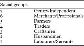
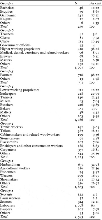
As previously noted, Clark's hypothesis rests on information concerning the wealth of individuals, which is unavailable in the Cambridge data set. We have, however, since Greg Clark kindly made the precise details of his classifications available to us, been able to map our occupations into the same seven social groups based on wealth as described in Clark and Cummins (Reference Clark and Cummins2010); see Table 2. A detailed breakdown of the composition of these groups is given in the appendix.
Social groups according to Clark and Cummins (Reference Clark and Cummins2010)

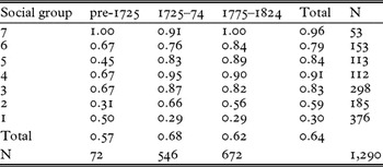
As described above, Clark characterizes the middle class in terms of values and wealth. The social groups are classified by wealth in ascending order. As to the values, the only variable we can observe is literacy. We measure the percentage of fathers who are literate, where an individual will count as literate if the marriage form was signed with the name instead of a mark.
Looking at the literacy rate by group in Table 3 reveals that the higher classes do indeed have a higher percentage of literate men, a pattern which is particularly clear when comparing the highest groups to the lowest. Partly with this is mind, we choose to focus on the differences between groups 6 and 7 and groups 1 and 2 for the remainder of this article.
Literacy rate by group

3. Survival of the richest?
This section uses the Cambridge data to reinvestigate the hypothesis advanced by Clark that wealthier families displayed higher fertility at a time when society was structurally static, and to examine the factors behind any differences in fertility between classes using information on age at marriage, length of reproductive period and spacing between the births of offspring.
3.1. Did wealthier fathers leave more children?
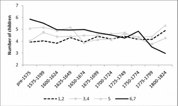
As discussed in the introduction, Clark argues that ‘middle-class’ families had persistently higher reproductive success before the Industrial Revolution than their lower-social-class counterparts (Clark Reference Clark2007). This is a relatively simple matter to investigate using the Cambridge data, and we do indeed find support for this hypothesis when looking at fertility levels for the different social classes, as Figure 3 illustrates.Footnote 5 For illustrative purposes, we have grouped the classes into four, and we have divided the sample into 25-year periods, within which we calculate the average number of children born to fathers who got married or had their first child within each particular 25-year period. The same periods are also used for the remaining results in this section.
Fertility by social group

Figure 3 shows that the wealthiest families, i.e. those in groups 6 and 7, gave birth to roughly one more child than their class 1 and 2 counterparts, especially at the beginning of the period, with groups 3 and 4 lying in between. Group 5, which is predominantly ‘farmers’, seems to follow a pattern more akin to the wealthier groups at the start of the period, and more like the poorer groups towards the end, which probably reflects the changing status of the word ‘farmer’ over this period.Footnote 6
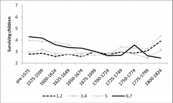
What ultimately counts for the hypothesis of value spreading, however, as was stressed by Clark and Hamilton (Reference Clark and Hamilton2006) and by Clark (Reference Clark2007), is not the number of children born to a family (gross fertility), but the number of surviving children, i.e. offspring who reach 15 years of age. Offspring who have no death date reported are counted as surviving offspring, following Wrigley et al. (Reference Wrigley, Davies, Oeppen and Schofield1997). This builds on the implicit assumption that children remain with their parents (who we know stayed in the parish) up until the age of 15. Figure 4 shows the number of children surviving by social class. Remarkably, Figure 4 is virtually identical to Figure 3,Footnote 7 with the wealthier families producing roughly one more surviving offspring than the poorest groups, where this difference is most prominent in the sixteenth and seventeenth centuries. Clark and Cummins (Reference Clark and Cummins2010), using a larger data set on testators, reach a similar conclusion, that wealthier testators were more successful in terms of reproduction until around 1780.
Reproductive success by social group

Interestingly, Figure 3 also reveals that the decline in the number of children born – one of the main components of the historical demographic transition – started much earlier among wealthier families than among the lower social classes. This led to a point where, by the nineteenth century, they were generally having fewer children than poorer groups in society, a finding supported by Clark and Cummins (Reference Clark and Cummins2009, Reference Clark and Cummins2010). A similar story, including the same spike in fertility at the end of the eighteenth century, has been documented for the British and Irish Quakers, a group that was certainly better off than average (Vann and Eversley Reference Vann and Eversley1992, pp. 132, 173).
It is also striking that the onset of the fall in fertility among middle-class families coincides with that of French families (Weir Reference Weir1994), where it also seems to have been the richest groups who reduced fertility first (Cummins Reference Cummins2009). The early fertility decline in France has been a great puzzle to scholars of demography, since it is difficult to explain why the fertility of the French declined before the fall in mortality. The Cambridge data point to the fact that England, at least among non-manual families, saw a pattern that was similar to that of the French.
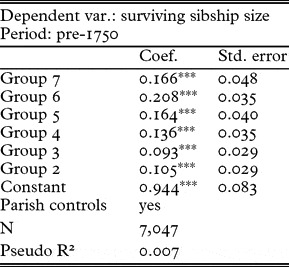
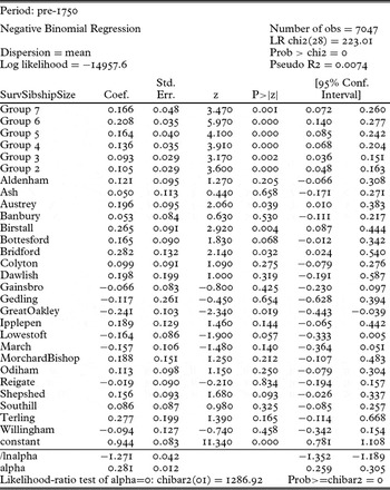
In order to test more formally whether the differences in reproductive success are statistically significant we conduct a regression analysis, regressing the number of surviving children on the social group of the father. The results are presented in Table 4. Since the relationship between wealth and fertility seems to change sometime in the eighteenth century, we limit our sample to the period before 1750. We control for differences owing to parish-level differences in net fertility by including parish dummiesFootnote 8 and the results are found using a negative binomial regression, to take account of the discrete nature of the dependent variable.
Regressing net fertility on social group for the period until 1750

*** significant at 1%
Clearly, all social groups have significantly more children than group 1, which is the reference category. It is also clear that there is no significant difference between the parameter estimates for groups 6 and 7 – justification for our aggregation of these groups in the figures above. To interpret the coefficients it is necessary to take the exponential function to the constant, in the case of group 1, or the constant plus the coefficient, in the case of the other six groups. So, for example, the expected number of children for a person in group 1 is e0.944 = 2.57, whilst for someone in group 6 it is e(0.944+0.208) = 3.17.
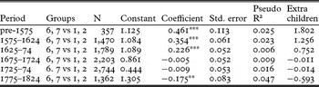
As was seen in Figures 3 and 4, however, the reproductive advantage of the wealthier classes does not last throughout the whole period. Table 5 illustrates the results of the same regression, but where we divide the data into 50-year periods. Since the focus of our work is to compare fertility of the wealthier to that of the poorer classes, we only report the coefficients of groups 6 and 7 as opposed to groups 1 and 2, as well as the number of additional children that groups 6 and 7 are predicted to have.
Regressing net fertility on social group by 50-year period

*** significant at 1% ** significant at 5%
As also indicated in Figures 3 and 4, groups 6 and 7 have more than one additional surviving child compared to groups 1 and 2 at the beginning of the period, but this difference becomes insignificant around 1700.
We also considered fertility differences by region within England, but we find no obvious systematic differences – a similar conclusion to that reached by Wrigley et al. (Reference Wrigley, Davies, Oeppen and Schofield1997), although in marked contrast to that presented by Vann and Eversley (Reference Vann and Eversley1992).
Summing up, the Cambridge data set confirms the first part of Clark's hypothesis, that wealthier social classes had more surviving offspring than their lower-class counterparts, although this only seems to hold true until the 1700s.
3.2. What explains fertility gaps between classes?
It is interesting to consider briefly how parents were able to regulate their fertility at a time of limited or no access to contraception.Footnote 9 Generally, demographers consider three main methods: delaying marriage (since most children were born within marriage), ‘stopping’ or the decision to stop having children before the menopause, and ‘spacing’, i.e. regulating time intervals between the birth of each child.
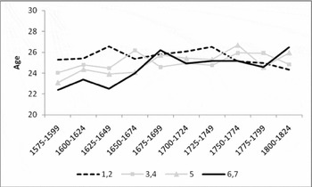
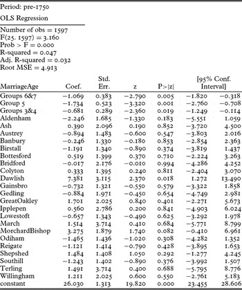
Figure 5 illustrates the mother's age at first marriage for 25-year periods. This clearly corresponds to the pattern we saw in Figure 3, since the groups with higher fertility simply got married earlier.Footnote 10 To begin with, these are the wealthier groups (based as usual on the occupation of the husband/father), but later these are the poorest groups. Regression results, reported in the appendix, confirm that this difference is statistically significant when looking at the period up to 1750. Note that we do not illustrate the pre-1575 period since here there are too few observations where we know the age of the mother (this is also the case for Figure 6, below).
Wife's age at first marriage

Wife's age at last birth

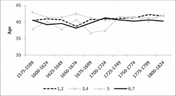
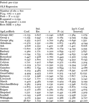
The fact that wealthier women got married two to three years earlier in the early years clearly prolonged the time span over which children could be born within marriage. Whether these parents, on average, fully enjoyed this as a longer fertile period, however, also depends on their ‘stopping behaviour’. As Figure 6 demonstrates, the age of a wealthier woman at the time of the birth of her last child was slightly lower than that of the poorer groups.Footnote 11 Prior to 1700, women in groups 6 and 7 on average had their last child at the age of 39.05 whereas women in groups 1 and 2 had their last child at the age of 40.2. However, statistically this difference is not significant. Thus, wealthier families did indeed experience a longer fertile period than less wealthy parents.
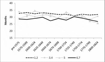
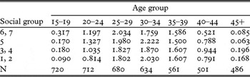
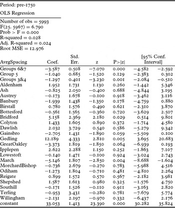
Finally, we look at the ‘spacing’ intervals as illustrated in Figure 7.Footnote 12 As expected, the wealthier groups have shorter intervals between consecutive births, thus allowing them to have more children over the same time span.Footnote 13 Rather than a conscious choice, these differences were likely to do with the fact that women's fertility declines with age. Hence, since women in the higher groups got married earlier, they were more fertile at any particular birth order compared to women of the lower social group. This is confirmed by Table 6, where the average number of children (gross) of women in five-year age groups is calculated. Clearly, women in higher social groups had more children earlier in life. Later in life the pattern seems to reverse, although it should also be noted that this calculation does not take mortality into account.Footnote 14 Another explanation could be that women in the poorer groups had to work physically harder, or simply suffered from deficient nutrition or sanitary conditions, thus increasing their risk of miscarriage (see Livi-Bacci Reference Livi-Bacci1977 for a discussion on the relationship between living conditions and fertility in Italy).Footnote 15
Average length of birth interval (in months)

Average number of children by woman's age group

In conclusion, it seems that the reason why wealthier groups gave birth to more offspring was that less time went by between each birth, and also the fact that they married earlier, where the latter might explain the former.
3.3. Did society remain static?
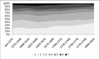
For middle-class values to spread throughout society, it was of course necessary that the middle classes were not closed or cut off from the rest of society. If society was socially static, meaning that the middle class's fraction of society was constant, or if their proportion was falling over time, then given that they also had higher fertility, this would imply that their children would be forced to work in lower socio-economic groups. Figure 8 illustrates the evolution of the relative size of each of our seven social classes over time.
Shares of social groups

It does indeed seem that the data support Clark's hypothesis of a socially static society, since the shares were relatively constant up until the end of the seventeenth century. The poorest groups, 1 and 2, comprise around 40 per cent of society, while the richest groups, 6 and 7, are at around 20 per cent. Perhaps not surprisingly, given what we know about the huge structural changes taking place in England during the Industrial Revolution, something changes from the eighteenth century. Specifically, and not unexpectedly, groups 1, labourers, and 3, craftsmen, are growing as a share of society. Regarding the growth in the latter, this seems to be consistent with the findings of Leunig et al. (Reference Leunig, Minns and Wallis2009), who showed that education grew in importance over this period, particularly in the form of apprenticeships requiring skills needed for manual labour, such as that used in manufacturing (van der Beek Reference van der Beek2010).
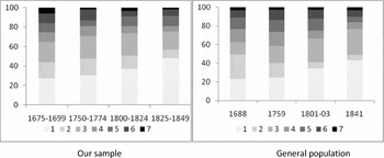
More worrying is the precipitous decline in the share of groups 6 and 7 towards the end of the period, which we think implies that our sample becomes less representative of the whole country as the professional classes moved out of the rural parishes documented by the Cambridge Group and into the towns. This is consistent with a comparison of the occupational structure we find with that from various other sources, as illustrated in Figure 9.
Representativeness of the data

The data for 1688 (Lindert and Williamson Reference Lindert and Williamson1982) are aggregated into rather broad occupational categories, and are thus difficult to classify according to our groups. But the data still look acceptably similar to ours. From this date we have the same trend in group 1 (labourers) and 3 (craftsmen) as in the general population. Both for the estimates of 1801–3 as well as the census data from 1841 we can see that groups 6 and 7 are underrepresented in our sample. Indeed, this could be due to these people increasingly moving to cities, where we would not be able to observe them. Thus, for the analysis of social mobility in Section 4 below, we concentrate on the period before 1750 where our data seem to be largely representative of the general population.
4. Memes or genes?
Clark's hypothesis and his findings, which by and large can be supported with our data, raise some important questions, about which Clark himself seems rather agnostic. Of course, as mentioned in the introduction, there is no way to test whether the values considered by him really did spread through society in the way he suggests. But we can consider how they might have done so, given that we know that the offspring of the richer classes did indeed move down through society. In considering this, we move more into the realm of evolutionary biology, which is somewhat beyond the scope of this article. Nevertheless, we feel that our findings have some important implications for this debate.
Two mechanisms have been suggested for the propagation of values through society. The first relates to the so-called Lamarckian view (after the French biologist Jean-Baptiste Lamarck 1744–1829), that an organism can pass on characteristics acquired during its lifetime to its offspring. In a social context this corresponds to the transmission of memes, a word first suggested by Richard Dawkins (Reference Dawkins1976) to provide a framework for understanding the evolutionary principles underlying the spread of ideas and cultural phenomena.Footnote 16 The second, perhaps more controversial, theory suggests that these values might be intrinsic to individuals, because they are encoded in their DNA. Many social scientists might shy away from this interpretation, associated as it is with the work of eugenicists in the 1930s, but in reality the evolutionary forces governing the spread of genes or memes are rather similar. Economists are, in fact, leading the way in reopening the debate about the role of genetics for society, starting with the pioneering work of Gary S. Becker (Reference Becker1976). More recently, this has become a growing area of interest for those working within the field of Unified Growth Theory, relying as it does on the development of preferences for quality as opposed to quantity of offspring (see Galor Reference Galor, Aghion and Durlauf2005, p. 231, and Galor and Moav Reference Galor and Moav2002). What can our results tell us about whether memes or genes might have governed the transfer of middle-class values?
The Cambridge data permit us the possibility of going one step further in addressing the issue as to what extent middle-class values were trickling down by middle-class children leaving the social class in which they were born, because for a subsample of our sample, we have information on the occupations of both fathers and sons. We can use this to construct social mobility tables, as commonly used in sociology. Because we know that our data become less representative as we move into the period of the Industrial Revolution, we perform our analysis until 1750, where the year applied is the birth-year of the son.
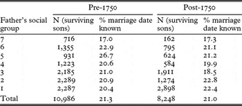
Looking at social mobility causes us to dwell a little more on a problem with our data which we mentioned briefly above: namely, that even if a father stays in the same parish, his sons might migrate when they become adults. This could bias our mobility results if the sons from fathers of one group had a greater chance of moving out of the parish than those of the other groups. To get an idea of whether this might be the case, Table 7 shows the number of surviving sons the couples in our subsample (where we know the occupation of the father) have and the percentage of sons observed for each social group. The idea is that if they stay in the parish and get married, we would be able to observe the son, so differences in the proportions in each group for which we know the marriage date of the son would indicate differences in the tendency of sons to move out of the parish.
Percentage of sons with marriage date observed

Fortunately, the percentages are similar at around 20 per cent for all groups, although we observe sons of group 7 slightly less often. This implies that group 7 will be slightly underrepresented in the mobility results. It is not clear whether these sons would follow the same mobility pattern as those staying in the parish, have a greater tendency to remain in group 7 or have greater downward mobility. This is not crucial to the results, but should be kept in mind when interpreting the results on intergenerational mobility for this group.
When examining social mobility tables, one should be aware of the fact that for the higher classes there is only the possibility of staying high in society or moving down, whereas the lower classes are only faced with the possibilities of staying low or moving up. The former is, however, exactly what we are looking for, namely the fact that the additional children of the higher classes had only one way to go. Taking this as a starting point, we are only interested in the degree of downward mobility of the higher classes and the degree of upward mobility into these classes.
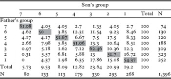
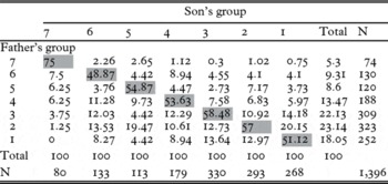
First, we look at outflow mobility: see Table 8. This shows us the destination classes of sons contingent on their father's social class. Diagonal numbers refer to the percentage of sons remaining in the social class of their fathers. From the row percentages, it can be seen that, on average, only around 50 per cent of group 6 fathers had sons remaining within the same group, with the remainder largely moving to lower groups. This was to some extent balanced by upward mobility into these classes (shown by the column percentages), but there is no escaping the fact that there was mainly downward mobility from the richer groups. This is in line with our previous results, that these groups had higher fertility at a time of a static social structure.
Outflow mobility (row percentages), pre-1750

It might be noted that the greatest mobility, in terms of both upward and downward mobility, was between groups 6 and 4, the non-manual occupations, in line with modern findings of a ‘buffer-zone’. This has been widely observed for Britain in more recent times, e.g. Heath and Payne (Reference Heath, Payne, Halsey and Webb2000) and Miles (Reference Miles1999), although this is most stringent when looking at relative mobility rates (relative to perfect mobility), as noted by Goldthorpe, Llewellyn and Payne (Reference Goldthorpe, Llewellyn and Payne1980). As for group 5, most mobility occurs with group 2, as could be expected taking into account that both of these groups concern agricultural occupations. Group 7 seems to be most persistent, with around 80 per cent of sons born in this group being able to stay. This is somewhat intuitive as this group is largely concerned with titles, rather than with occupations. Nevertheless, here we also observe that downward mobility, especially to the lowest groups of labourers, is generally larger than upward mobility of these groups into group 7.
Although we have now demonstrated that there was indeed downward mobility from the richer groups, it is important also to consider patterns of inflow mobility, i.e. where the members of each group came from, as shown in Table 9. This is crucial for understanding the impact potential of this downward mobility. As can be seen, only around 5 to 10 per cent of groups 1 to 5 came from groups 6 and 7, whereas around 50 per cent of group 6 and around 20 per cent of group 7 came from lower income groups. This reflects the fact that, despite the downward mobility from the richer groups, they were a relatively small share of the population,Footnote 17 so their impact on the other groups was fairly minor. On the other hand, small movements from the lower income groups had a large impact on the higher income groups.
Inflow mobility (column percentages), pre-1750

What does this imply for the idea that middle-class values were spreading through society? Leaving aside the question of whether groups 6 and 7 really did reflect the values which Clark associates with the middle class, it is difficult to draw clear conclusions. The mobility into lower groups was certainly rather little in relation to the large size of these groups, and besides, many were moving up the other way. However, it could be the case that the great mobility of English society could lead to a demonstration effect, whereby other socio-economic groups learnt by example from the offspring of the rich. On the side of the genetic argument, even a small reproductive advantage could cause certain individuals to dominate if their genes were being mixed into all tiers of the population over a long enough period of time.
In both cases, it was the great mobility of English society which could have given rise to the sort of phenomenon Clark suggested, but we are still not much closer to knowing whether it really did happen. The changing view of genetics amongst modern biologists does not make the job any easier. A rather brief foray on our part into the recent literature shows that the general belief that genetics somehow determines phenomes (i.e. appearance, physiology, behaviour etc.) is incorrect. What is known as developmental plasticity means that genes can be ‘activated’ or ‘deactivated’ depending on environmental conditions.Footnote 18 The implications of this are rather profound. It might well have been the case that certain attributes began to be favoured in the English population prior to the Industrial Revolution, but was this due to genetic or memetic mutation and reproductive success, or simply due to the activation of certain genes given new environmental conditions? If the latter was the case, the differing reproductive success of social groups becomes an interesting statistical finding, but perhaps of little or no long-run practical importance whatsoever.
One final point: much interesting work has been done recently on historical social mobility, and it is natural to compare our results with this. Generally, the levels of social mobility in Britain found for the nineteenth century are considered to be rather low, although increasing again in the twentieth century (see, for example, Ferrie and Long Reference Ferrie and Long2010). Our evidence suggests a longer story of high but decreasing social mobility before the nineteenth century, although much needs to be done to make our work fully comparable to studies of more recent years, where the methodology and the classification of socio-economic groups is usually rather different. There remains in fact plenty of room for more research based on the evidence from the Cambridge data, not just in extending this analysis to the period after 1750, but also in investigating intra-generational mobility, since we sometimes have observations for one individual of both occupation at marriage and at death (see the work from the nineteenth century by Long Reference Long2010).
5. Conclusion
This study offered an attempt to investigate the notion forwarded by Greg Clark that the spread of middle-class values to lower social classes, through social mobility, might have been a stimulus to England's Industrial Revolution. We used data from the Cambridge Group's population history of England from family reconstitution to carry out two specific analyses required to test Clark's hypothesis. One was to find out whether middle-class families were more successful in terms of reproduction than their lower-social-class counterparts. The other was to test if pre-industrial England was socially static over time. According to the Cambridge data, both were true up until sometime in the eighteenth century.
Acknowledgements
We would like to thank the Cambridge Group for making their data available to us, and Gill Newton for help with clarifying questions. We are grateful to Marc Klemp for preparing the data for the analysis. We thank Tommy Bengtsson, Greg Clark, Martin Dribe, Marc Klemp, Markus Lampe, Karl Gunnar Persson, Leigh Shaw-Taylor, the editors and referees of the European Review of Economic History and participants at the Copenhagen FRESH meeting and the 5th Sound Economic History Workshop in Lund for valuable comments and suggestions. Jacob Weisdorf also thanks the Robert Schuman Centre for Advanced Studies at the European University Institute for its financial support through a Jean Monnet Fellowship, and Paul Sharp would like to thank the Carlsberg Foundation for their financial support.
Appendix
Main occupations in social groups

Regression results: surviving sibship size

Regression results: marriage age

Regression results: mother's age at last birth

Regression results: average spacing