


For virtually all of the lifetimes of the present authors, realignment theory a la Key (Reference Key1955, Reference Key1959) has been a central component of the common wisdom shared by students of American politics (see especially Burnham Reference Burnham1970; Sundquist Reference Sundquist1983). A key aspect of many variants of realignment theory is a claim that there are important periodicities to patterns of realignment. For example, Arthur Schlesinger, Jr. (Reference Schlesinger1986) reports his father's famous prediction in a 1924 lecture that “Coolidge-style conservatism would last till about 1932,” his further prediction (Schlesinger Reference Schlesinger1939) that the “prevailing liberal mood would run its course in about 1947,” and later in 1949 that the “recession from liberalism was due to end in 1962,” and that the “next conservative epoch will commence around 1978.” That these predictions of mood changes about every 15 years were on target not only reflects the elder Schlesinger's understanding of history but also suggests that somewhat regular cycling of political dominance may occur, or as his son puts it, “Predictive success creates a presumption in favor of a hypothesis” (Schlesinger Reference Schlesinger1986). Overall, the Schlesinger predictions suggest a cycle length—the time for the state of the political system to return to a given position—of about 30 years.
That and similar numbers took on an almost sacred significance in most subsequent realignment literature. Mayhew (Reference Mayhew2002, 16) quotes Burnham (Reference Burnham, Chambers and Burnham1967), who suggests that “a realignment cycle emerges once every thirty years”: or “approximately once a generation, or every thirty to thirty-eight years.” Beck (Reference Beck and Niemi1974) suggests that “Realignments have occurred at roughly three-decade intervals. . ..” Although what Burnham means by a “realignment cycle” is not entirely clear—because in his historical examples, the party achieving ascendancy on consecutive realignment dates is sometimes the same party and sometimes a different party—his emphasis on realigning elections suggests that his “cycles” correspond to durations of party ascendancy and thus represent only one half of a true cycle in which the system returns to its previous state, after passing through periods of dominance by each party. It is this latter meaning of “cycle,” as applied to partisan dominance, that is used in this study.
In this paper we take up a variety of issues related to the periodicity of realignments. Are there cycles in American politics? Specifically, does the proportion of, say, the Democratic vote/seat share rise and fall over extended periods of time or, on the other hand, is change more or less random? If there are such cycles, are they regular; that is, does the system return to the same state at regular intervals? If so, what is that interval, and is it the same or different for the House, the Senate, and the president? Perhaps most importantly, if there are regular cycles, can we identify the forces that drive that behavior? In particular, can we construct an integrated model—such as a negative feedback loop—that generates the observed patterns?
It is important to try to pin down exactly what it is that is supposed to be exhibiting cycles. In fact, there have been at least five distinct notions of realignment. One approach defines a realignment as occurring (1) when there is a change in party dominance, or, in Lubell's apt metaphor (Reference Lubell1952), a change in which party is the “sun” and which the “moon” of politics. A second approach also looks at dominance, but at (2) change in the dominance of ideological orientations (such as conservative versus liberal: Schlesinger, Sr., Reference Schlesinger1939; Schlesinger, Jr. Reference Schlesinger1986; or ideals versus institutions: Huntington Reference Huntington1981) rather than parties, per se. A third approach (often associated with Key (Reference Key1955, Reference Key1959) focuses on (3) substantial change in the composition of each party's sociodemographic support base. The fourth approach, associated primarily with political geographers (Shelley and Archer Reference Shelley and Clark Archer1994; but see also Nardulli Reference Nardulli1995), emphasizes (4) change in the geographic loci of party support, especially in regional terms. The fifth, associated most with the work of Schattschneider (Reference Schattschneider1960, Reference Schattschneider1988) and then Riker (Reference Riker1982), treats realignment as (5) a change in the defining issue cleavage(s) that structured political competition.
Scholars who have emphasized realignment cyclicity tended to focus on the first two of the five approaches to defining realignments identified above. Although most of the literature looked (a la Lubell) at evidence for alternation of parties in power, there were also those who (like Arthur Schlesinger, Sr.) were concerned more with ideological dominance. As noted earlier, Arthur Schlesinger, Sr., took his cyclical swings to be between what he identified as conservatism and liberalism, not as between the two major political parties. Another approach to periodicity, involving a dichotomy between “private interest” and “public action,” was identified by Hirschman (Reference Hirschman1982) and adopted by Arthur Schlesinger, Jr. (Reference Schlesinger1986). The latter finds alternation in the dominance of these two poles of a policy orientation spectrum largely independent either of the business cycle or of the foreign policy cycle (between “introversion” and “extroversion”) identified by Klingberg (Reference Klingberg1952, Reference Klingberg, Kegley and McGowan1979). One suggestion of what might drive cycles comes from Arthur Schlesinger, Jr. (Reference Schlesinger1986, 28):
Disappointment [is] a basic spring of political change. People can never be fulfilled for long either in the public or the private sphere. We try one, then the other, and frustration compels a change in course. Moreover, however effective a particular course may be in meeting one set of troubles, it generally falters and fails when new troubles arise. . .. As political eras, whether dominated by public purpose or private interest, run their course, they infallibly generate the desire for something different.
Closely related to the question of why we might get cyclic patterns is the question of the structure of cyclic change. A voluminous literature—initiated by Lubell (Reference Lubell1952; see also, e.g., Key Reference Key1959; Burnham Reference Burnham, Chambers and Burnham1967, Reference Carmines, Stimson, Dalton, Flanagan and Beck1970; Sundquist Reference Sundquist1983; Beck Reference Beck and Niemi1974) supports a concept of realignment under which control of politics by a majority party reaches a breaking point culminating in a crucial event leading to change in the composition of the parties, that is, a realignment. These authors speak frequently of “critical” or “defining” elections that alter the political balance of power abruptly, achieving a new state that is sustained over a number of subsequent elections. Furthermore, Burnham (Reference Burnham1970) states that “. . . national critical alignments have not occurred at random. Instead, there has been a remarkable uniform periodicity in their appearance.”
The 1960s and after, however, did not seem to fit a realignment model that focused primarily on “critical” realigning elections. By the strong criteria usually required for an election to be labeled “critical,” no realignment occurred in the 1960s when, by the every 30 years or so expectation, one was due. A variety of terms were coined to describe the post-1960s era: “dealignment,” “stalled realignment,” “post realignment” (see various essays in Shafer Reference Shafer1991 and subsequent works too numerous to mention). But, arguably, it was not until Mayhew's (2002) book-length challenge to the common wisdom about realignment theory that the assertion was unambiguously made that the periodicity hypothesis was wrong.
Mayhew (2002) offers a detailed history and critique of the scholarly literature that argues for the existence of regular patterns in American historical politics. We fully agree with Mayhew that discussion of cycles has been long on rhetoric and anecdotal evidence and short on rigorous statistical analysis and the development of explanatory models. But Mayhew's discussion of the statistical evidence bearing on the existence of cyclic patterns in party strength relies too heavily on one particular statistical analysis, by Gans (Reference Gans1985; see Mayhew, 149), which simply does not have the negative implications claimed for it—as we show below. More importantly, the data we analyze here on the aggregate support for each party over the period 1854–2006—using statistical methods appropriate for identifying periodicities—does show evidence for gradual, but regular cyclical change.
Sustained realignments following critical elections are quite different from gradual (but still cyclic) changes in the level of support for each party—a pattern more in line with the approach taken by the Schlesingers (Reference Schlesinger1939, Reference Schlesinger1986; see also, Carmines and Stimson Reference Carmines, Stimson, Dalton, Flanagan and Beck1984). As we will see, it is the latter pattern that is supported by our empirical evidence. We do not find overall support for the abrupt changes implicit in the concept of critical elections—although we recognize that some abrupt transitions have occurred. And the formal feedback model we offer below is one that is compatible with this latter pattern of cyclic change.
CYCLING IN THE PARTISAN SHARE OF SEATS/VOTE 1854–2006: THE EMPIRICAL RECORD
Time-Series Plots
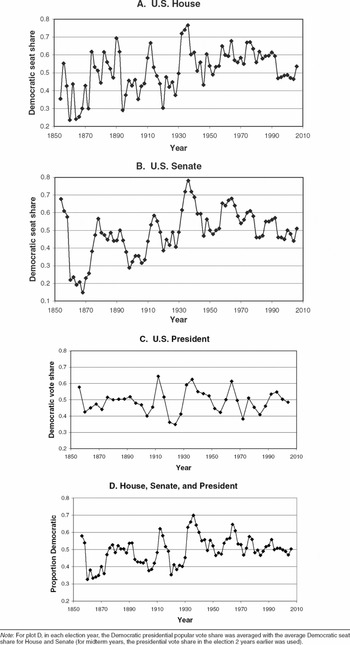
In Figure 1, we present time-series plots over the period 1854–2006, which encompasses the full historical period to date of American politics dominated by the Democratic and Republican parties. The plots in Figure 1A and 1B depict the variables House and Senate that represent the proportion of Democratic seats for the U.S. House of Representatives and for the U.S. Senate, respectively; Figure 1C plots the variable President, that is equal to the proportion of the major party popular vote received by the Democratic nominee for the presidency.Footnote 1Figure 1D summarizes this information by plotting the variable House, Senate, and President, which is the average of the Democratic share between the variable President and the average of the variables House and Senate.Footnote 2
Historical Time-Series for American Politics

Are Partisan Shifts Random?
Before considering vote or seat share, we simply track who wins. The simplest hypothesis for the pattern of Democratic and Republican wins in either the presidency or the houses of Congress is a simple binomial trials model. This is equivalent to assuming that winning is random and equally likely for the two parties. To test this model we can perform runs tests on data for the period under study. A run constitutes a sequence of consecutive elections in which the same party wins (i.e., wins the presidency or wins a majority of the seats in a house of Congress). For example, during the period 1984 to 1996, Senate majorities can be represented as RDDDDRR, where D denotes a Democratic majority and R denotes, a Republican majority. During this period there were three runs, that is, R, DDDD, and RR. Note that the number of runs in a period is always one more than the number of switches between parties, so effectively testing runs is equivalent to testing partisan switches. If a sequence of N elections represents independent, binomial trials each with probability 0.5, then the expected number of runs is (N + 1)/2.
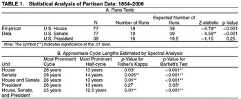
For presidential elections over the period 1856 to 1980, Gans (Reference Gans1985; cited also by Mayhew 2002, 149) reports a runs test that finds no significant difference in the number of runs from what we would expect in an independent binomial trial. Our runs test for presidential elections (for a slightly longer historical period) is consistent with Gans's result. Evidence from data on presidential run lengths is interpreted by Gans (and by Mayhew) as strong evidence against cyclic notions of realignment. But, as we show below, this is not a statistically appropriate conclusion. Moreover, when we perform similar runs tests for House and Senate elections over the 1854 to 2006 period, we find compelling evidence that longer runs of party control occur than would be expected by chance alone (Gans also did unspecified runs tests on congressional data but did not regard them as informative). For House, Senate, and presidential elections, Table 1A gives the number of runs, expected number of runs under the independence assumption, and the p-value for the runs test of the null hypothesis that the time series is a sequence of independent binomial trials.Footnote 3
Statistical Analysis of Partisan Data: 1854–2006

Note: The symbol (*) indicates that the test statistic is significant at the .05 level; the symbol (**) indicates significance at the .01 level. Fisher's Kappa statistic tests whether the largest amplitude in the periodogram (which represents the most prominent period) differs significantly from the mean amplitude. Bartlett's Kolmogorov-Smirnov statistic tests if the time series is distinct from white noise.
It is clear that both the House and the Senate have far fewer runs (i.e., fewer partisan switches) than would be expected if members were elected independently of each other and over time.Footnote 4 For presidential elections, there are slightly fewer runs than would be expected under independence, but not significantly so.Footnote 5 Why are results different for presidency and Congress? One obvious possibility is that the presence of incumbency effects in Congress changes the nature of cyclic dynamics, in that incumbency effects slow change in party control. But an adequate interpretation of the failure to reject the null hypothesis for the presidential time series lies deeper. The statistical power of the runs test to distinguish random from cyclical behavior is much too low for the test to be meaningful.
To see this, note that the fact that the hypothesis of randomness leads to an expected number of runs on the order of N/2 does not preclude other hypotheses leading to the same expected number of runs. Suppose, for example, that a time series were perfectly cyclical, following a sinusoidal curve with period of 24 years.Footnote 6 With presidential elections every 4 years, there would be six elections and two partisan switches in each cycle, so the number of runs would be approximately (2/6)N = N/3. On the other hand, if we assume that incumbency guarantees reelection for a second term for a total of 8 years, there would effectively be three elections per cycle but still two partisan switches, so that in this latter case the number of runs would be approximately (2/3)N = 2N/3. Thus, with a sample size of 38 and a significance criterion of 0.05, the runs test lacks the power to distinguish either of these models from pure randomness (for which the expected number of runs is about N/2).Footnote 7 In other words, a key piece of statistical evidence that is relied on by Mayhew (2002) and others to disprove the existence of cycles does not have the meaning commonly attributed to it.
Next we look at the question of periodicity of aggregate U.S. presidential and Congressional time series within a more sophisticated statistical framework.
Spectral Analysis Periodograms
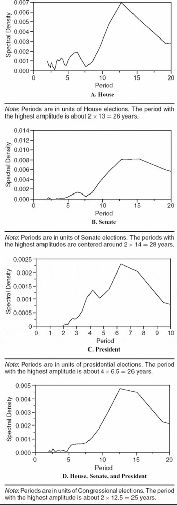
In order to investigate the possibility of cycles in historical time series, we perform a spectral analysis—a procedure that decomposes the pattern over time into a spectrum of cycles of different lengths, just as a prism decomposes white light into a spectrum of colors of different wavelengths or frequencies (Bloomfield Reference Bloomfield2000). The output of such an analysis is conventionally represented by a periodogram, a plot that emphasizes the dominant frequencies (or, alternatively, cycle lengths) that make up the time series spectrum. Specifically, a periodogram plots on the Y-axis the squared amplitude corresponding to a cycle length against that cycle length on the X-axis, that is, the relative strength of the contribution of each associated frequency to the overall pattern of the time series.Footnote 8 The peaks in the plot represent the strongest frequencies in the (Fourier) decomposition of the time series; reciprocals of these frequencies represent the corresponding strongest periods or cycle lengths reflected in the time series.
Because the time series is recorded every 2 years (or every 4 years in the case of the presidential series), each of these cycle lengths must be multiplied by 2 or 4, respectively, to obtain cycle lengths in years. Note that a “period” represents a complete cycle, such as a duration of Republican ascendancy plus a duration of Democratic ascendancy, that is, the time for the political landscape to return to a specified state. Hence the average duration that one party is in power is half a period as defined by the periodogram. Note that each position on a periodogram integrates information equally from the entire historical period. The x coordinate represents a cycle length (reciprocal of a frequency), whereas the y coordinate represents how strongly that cycle length is reflected in the pattern shown by the data.
For example, the highest peak in the periodogram for the Democratic share of the House occurs for a cycle length of about x = 13 House elections, or about 2×13 = 26 years. In turn this means a shift from one party to the other, on the average, about every 13 years. Of course, this represents an average and is approximate; among other things, any particular shift would in fact occur after an even number of years. But overall, the plot suggests that there is more evidence of a cycle of about 26 years than cycles of any other period.
The half-cycle of about 13 years—that represents the duration of each party's ascendancy before dominance shifts to the other party—is very different from the 30-odd-year duration that is often posited in the realignment literature typified by Burnham (Reference Burnham1970) and Beck (Reference Beck and Niemi1974) as the period between realignments and hence the period of one-party ascendancy. In particular, it is the half-period of 13 years, not the 26-year period, which is to be compared with 30+ years suggested by the realignment literature.
The periodograms are presented in Figure 2.Footnote 9 For each of the partisan measures, the durations of the most prominent periods (in years) are indicated in Table 1B, as estimated from the periodograms: about 26 years for the House, approximately 28 years for the Senate, and about 26 years for the president. So the Senate may be the slowest of these three institutions in terms of response time. Given the staggered nature of Senate elections, with just a third of the seats in the body up in any given election, this observation makes sense. Beyond this small possible difference, however, the consistency over institutions of the primary period in the vicinity of 25 to 30 years is striking.
Periodograms for Measures of Democratic Party Strength: 1854–2006

Two hypothesis tests were performed on the periodograms. Fisher's Kappa statistic (Fuller Reference Fuller1996) tests whether the most prominent period observed is statistically significant, by determining whether the largest amplitude in the periodogram (which represents the most prominent period) differs significantly from the mean amplitude. The Fisher's Kappa tests for the House, the Senate, the House and Senate, and for the House, Senate, and President are each significant at the .05 level; the tests for the Senate and for the House and Senate are also significant at the .01 level. Only the test for the President alone (for which fewer data points are available) is not significant: p = 0.27. Second, Bartlett's Kolmogorov–Smirnov statistic (Fuller) tests whether the time series is distinct from pure randomness, by computing the absolute distance between the cumulative periodogram and the cumulative distribution for a uniform distribution (the latter represents the expected value for white noise). All Bartlett's test statistics were significant at the .05 level, and all but that for President at the .01 level. It is not surprising that the statistical results for the presidential time series are less strong than those for the Congressional series. Not only are there only half as many data points; but also the presidential series is perturbed by support for individual candidates with varying perceived qualities such as competence and charisma—an effect that tends to average out in determining Congressional seat share. Later we further assess the relative strength of evidence for cycling between presidential and Congressional data.
We turn now to the development of a dynamic model that represents our attempt to demonstrate that a simple negative-feedback loop involving only one dimensional political competition can generate the evidence for cycling that we have discussed above, and thus may account for an important feature of American political history.
ACCOUNTING FOR CYCLING: A VOTER–PARTY INTERACTION MODEL
We develop a dynamic model, based on interaction between voters and parties, in an attempt to account for the presence of regular cycling in American politics. In doing this we also consider the possible effects of incumbency advantage, the proportion of competitive seats, and changes in the voter distribution.
To our knowledge, the most extensive previous modeling of change in partisan vote share in American politics is based on the partisan business cycle (see Alesina, Londregan, and Rosenthal Reference Alesina, Londregan and Rosenthal1993; Alesina and Rosenthal Reference Alesina and Rosenthal1995), although single-equation studies of elections have been done by Erikson (1989) on presidential voting and Alesina and Rosenthal (Reference Alesina and Rosenthal1989) and Erikson (Reference Erikson1990) on voting in the House. The partisan business cycle is a joint, dynamic model of presidential and House elections that incorporates effects of economic growth (increase in real GNP) on presidential elections (but not directly on those in the House) as well as feedback between presidential and House elections. Alesina and Rosenthal (Reference Alesina and Rosenthal1995) fit this model to data for the period 1915 to 1988 and employ simulation to show that it can predict an equilibrium pattern of regular cycles. The Alesina–Rosenthal model does not directly involve spatial (policy) positioning of parties, although they present it in conjunction with their theory of institutional balancing that does use spatial modeling. Their model does not assume that parties have either a Downsian attraction (Downs Reference Downs1957) to the median voter on the one hand, or a policy-oriented motivation on the other.
Stokes and Iversen (Reference Stokes and Iversen1962) suggest several forces in addition to movements of the business cycle that tend to restore rather than disrupt partisan balance, including greater voter response to governmental mistakes than successes, ability of an out-party to make more flexible and extravagant promises, vulnerability of the in-party to splits as its majority grows (Riker Reference Riker1963), alternating moods of liberalism and conservatism, and a popular belief in rotation in office. Stokes and Iversen construct a model to show that, in both presidential and Congressional elections, restoring forces in some form are almost certainly present by effectively rejecting the hypothesis that the electoral trajectory has been a symmetric random walk (with draws taken from an empirical distribution of shifts in partisan support).
First we explore whether effects looked at one at a time are adequate by themselves to account for regular cycling. For example, one might suspect that cycling is due to the capacity of incumbents to retain office in a legislative body or for an incumbent party to retain the presidency. Computer simulations reported on our Web site (http://course.wilkes.edu/merrill/), however, suggest that, although incumbency may play a significant role in cycling, it alone does not appear adequate to account for regular cycling.
For a legislative body, a second possible explanation of regular cycling involves the proportion of seats that are competitive. We might expect that noncompetitive seats—those that are predictably and lopsidedly won by one party or the other—could lend stability to partisan divisions and hence lengthen cycles. But the basic effect of noncompetitive seats is to take a portion of the seats out of play. Variation in the partisan makeup of Congress depends on the remaining competitive seats. Fewer competitive seats correlate with a reduced swing ratio, but the likelihood that a legislative body will switch from majority Democratic to majority Republican or vice versa is not greatly affected by the number of seats that are truly competitive (or by the size of the legislative body). Hence, the proportion of competitive seats cannot be the sole explanation of regular cycling in a legislature.
A third potential explanatory factor—relevant to either legislative bodies or executive offices—is change in the voter distribution, sometimes referred to as tidal change. It is easy to see that periods in which voters prefer one party or the other will tend to lead—other things being equal—to corresponding periods in which the favored party holds legislative majorities and retains the presidency. Hence vote-driven tidal swings may tend to lengthen cycles, but our simulations show that accounting for regularity in the lengths of cycles requires additional forces in the model.
We turn now to a model that integrates several factors to account for regular cycling.
The Voter–Party Interaction Model
For simplicity, we consider a one-dimensional spatial model of electoral competition and assume that parties and candidates have policy-seeking motivations. Thus, each party or candidate faces a tradeoff between, on the one hand, advocating policies near its ideal point representing a preferred policy position that it can hope to implement if elected and, on the other hand, positioning itself nearer the median voter (in its constituency) in an effort to enhance its chances of being elected. Accordingly, there are centripetal as well as centrifugal forces influencing party and candidate position.
We postulate four principles for the interaction between the electorate and the political parties and candidates.
First, we assume each party (and its candidates) has policy motivations to move toward its ideal point over time (a centrifugal force).
Second, in its desire to win election, each party (and its candidates) is willing to move incrementally from its present position in the direction of the median voter position by an amount that is proportional to its distance from the median voter (a centripetal force).Footnote 10 This tradeoff is embodied in equations 1–2 below.
Third, the party in power (and in particular its individual candidates) enjoys an advantage in the next election that is independent of the spatial distance between party and voter positions (see equation 3 below). An in-party's advantage in a legislative body stems in part from its greater capacity to attract campaign contributions and other support and in part from the incumbency advantages of its individual members, which in turn derives from seniority, constituent service, visibility, and other factors. The in-party advantage in the presidency may depend on a general tendency to “support the president” and to “not change horses in midstream”—especially in good economic times.
Fourth and finally—in line with the insight articulated above by Arthur Schlesinger, Jr., but in counterpoint to the effect of the third principle—we assume that voters—at least near the center of the voter distribution and hence the median voter—move away from the position of the party in power, by an amount proportional to the distance between the median voter and the party's position (see equation 4 below). In other words, swing voters including the median voter may react negatively to policies implemented by the party in power. This assumption reflects observations of a number of scholars, including those of Stokes and Iversen outlined above. Samuels (Reference Samuels2004) provides empirical evidence that incumbents tend to lose vote share over time, and Bartels and Zaller (Reference Bartels and Zaller2001, 17) suggest that the longer the out-party is out, the more likely it is to nominate appealing candidates and offer reasons why voters may react over time to the party in power:
The longer an incumbent party has been in power, the more likely it is that political innovators will give way to less skillful successors (for example, Eisenhower to Nixon, Reagan to Bush, and Clinton to Gore). Seasoned advisers are likely to burn out and be replaced by second-stringers. Scandals tend to accumulate, as with the “corruption” of the Truman era, Watergate, Iran-Contra, and the various scandals of the Clinton years culminating, eventually, in the president's impeachment. Meanwhile, “easy” issues are likely to be dealt with and disappear from the political agenda, leaving increasingly intractable problems and increasingly disaffected constituency groups.. . .
Stimson (Reference Stimson2004, 165) makes explicit the pendulum swing in public mood:
Liberalism and conservatism in public preferences rise and fall in concert, the public changing its attitude toward government action in environment, welfare, urban aid, race, education, defense spending, and other issues all at the same time. This common national mood we know responds thermostatically to government policy. Mood becomes more conservative under liberal governments, more liberal under conservative regimes.
Stimson's observations not only suggest that voters respond with negative feedback to governmental action but also that response is coordinated over issues,Footnote 11 so that use of a one-dimensional spatial model may not be too far off the mark.
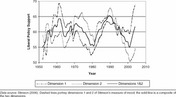
This observation by Stimson is supported by evidence he has amassed from nearly 200 surveys assessing voters' preferences on a wide range of issues. These preferences have been consolidated into two latent dimensions by Stimson. The first of these dimensions represents primarily economic issues while the second represents cultural issues. In Figure 3 we present plots, based on data from Stimson Reference Stimson2006, that track voter support for liberal policy from 1954 to 2004 on each of these dimensions and on a combined index that averages the two. We note that liberal policy support increases during the Eisenhower administration, decreases during the following Kennedy–Johnson terms of office and again later during the Carter administration, increases during the Reagan–Bush years, and decreases while Clinton was in office, only to increase once again during the second Bush administration. Thus, it is clear that, except perhaps for the Nixon–Ford years, support for liberal policy has increased during Republican administrations and decreased during Democratic administrations. This finding supports our fourth assumption—an assumption involving voter reaction to the policy of the party in power (see also Grofman Reference Grofman1985).
Liberal Policy Support (Stimson Mood) 1952–2004

Alesina and Rosenthal (Reference Alesina and Rosenthal1995) also suggest that voters react, but that they attempt to implement their reaction through another avenue; these authors assume that voters try to moderate the policies implemented by a partisan administration by voting for the opposite party for Congress at least in off-year elections. More generally, Fowler and Smirnov (Reference Fowler and Smirnov2007) suggest—using modern terminology—that moderate voters—even, for example, slightly conservative ones—may vote against a conservative president (or a conservative candidate expected to win the presidency) to dampen his or her mandate. Thus, under the Fowler and Smirnov assumptions, the voters behave as if the median voter has shifted away from the position of the president (or the candidate most likely to be elected president).
We assume that there is uncertainty about the location of the median voter (Wittman Reference Wittman1983); specifically the median voter is represented by a probability distribution. We introduce the following notation:
P R = Preferred (ideal) position of the Republican party.
P D = Preferred (ideal) position of the Democratic party.
M(t) = Expected value of the median voter distribution at time t.
R(t) = Position of the Republican party at time t.
D(t) = Position of the Democratic party at time t.
For simplicity of exposition, we speak of movements relative to the median voter to denote movements relative to the expected value of the median voter distribution. As the parties attempt to resolve the tension between their incentives to win vote share by moving toward the median voter while at the same time advocating their preferred policy positions, the party movements may be modeled as

and

where the terms M(t) − R(t) and M(t) − D(t) represent the signed distance from the expected median voter position to the party position, α is the median convergence parameter, and β is the party policy-motivation parameter. Note that, because of uncertainty about the location of the median voter and because of each party's policy-seeking motivations, neither party is motivated to jump to the expected location of the median voter.
We assume for presidential elections that the Democratic vote share is the proportion of voters who are nearer the Democratic position, plus an in-party effect that aids Democrats when the model projects that they hold the presidency and detracts when they do not. Similarly, for each chamber of Congress, the Democratic seat share is assumed determined by the proportion of voters who are nearer the Democratic position, plus an in-party effect that aids Democrats when—according to the model—they constitute a majority in that chamber and detracts when they do not. Specifically, the (expected) Democratic vote/seat share in the (t + 1)st election is the quantity E(t + 1) given by
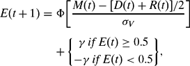
where γ is the in-party advantage parameter (which may vary over branches of government) and σV is the standard deviation of the voter distribution. We assume that the voter distribution is normally distributed and that Φ denotes the standard cumulative normal distribution function.Footnote 12 In the basic model we do not consider interaction effects between the chambers of Congress or between the president and Congress (but see the discussion below). Finally, the movement of the median voter away from the position of the incumbent party is modeled as

where δ is the voter reaction parameter and
![$
\begin{array}\[
W(t) = \left\{{{\begin{array}{@{}c@{}}
{D(t)\;\hbox{\it if}\;E(t) \ge 0.5}\\[4pt]
{R(t)\;\hbox{\it if}\;E(t) < 0.5}\\
\end{array}}} \right\},
$](https://static.cambridge.org/binary/version/id/urn:cambridge.org:id:binary:20151024010942576-0036:S0003055408080064_eqnU1.gif?pub-status=live)
so that the term W(t) − M(t) represents the signed distance from the incumbent party's position to the (expected) position of the median voter. The basic (deterministic) Voter–Party Interaction Model is defined by equations 1–4. We set the party ideal positions to P R = −1 and P D = 1.Footnote 13 The fact that, in the model, voters move away from the policy of the dominant party implies that in particular the median voter moves in this fashion, so micro-level behavior implies corresponding macro-level behavior. Equation 3 implies that voters choose the party with the more proximate policy position, but with a bias toward the incumbent. In turn, this has implications for macro-level behavior vis-à-vis the proportion of voters choosing each party.
To summarize, the model involves four parameters:
α = median convergence parameter
β = party policy-motivation parameter
γ = in-party advantage parameter
δ = voter reaction parameter.
We note that, as long as there is at least some voter reaction to the policy positions of the winning party, the only equilibrium in which the party positions remain unchanged over time occurs if both are at the mean of the median voter distribution and this position cannot change over time. For, if party positions are fixed, then R(t + 1) = R(t) and D(t + 1) = D(t). It follows from equations 1 and 2 that α [M(t) − R(t)] = − β [P R − R(t)] and α [M(t) − D(t)] = − β [P D − D(t)], so that R(t) =  and
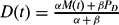 . In turn, if R(t) and D(t) do not change, M(t) must be constant, so that by equation 4, either the voter reaction parameter δ = 0, in which case there is no voter reaction to the policy positions of the winning party, or the winning party is at the mean of the median voter distribution, which is unchanging.
Extensions of the model to subnational units such as states or regions, to other polities, including the multiparty case and types of electoral rules other than plurality, are topics for future work. There has already been some work, using other models, along these lines. Lebo and Norpoth (Reference Lebo and Norpoth2007, 72), for example, suggest that “the swing of the electoral pendulum is as British as ale and kidney pie.” Although their principal objective is forecasting rather than cycling, they estimate a cycle length—using a second order autoregressive model for the period since 1929—of about five British elections, which works out to an average length of about 19 years per cycle. Norpoth (Reference Norpoth, Dorussen and Taylor2002) estimates a similar autoregressive model for the American presidential vote share for the period 1828 to 2000, but his estimate of a cycle length (about 20 years) is based not on the model but on the number of switches between Democratic and Republican majorities of the major-party vote, a measure that tends to overemphasize temporary reversals of power. Jerome, Jerome-Speziari, and Lewis-Beck (Reference Jerôme, Jerôme-Speziari and Lewis-Beck2007) find evidence for joint cycles in 15 European nations, although for only a 28-year period, based on economic variables and the politics of integration.
MODEL PROJECTIONS
Model Fit to Empirical Time Series
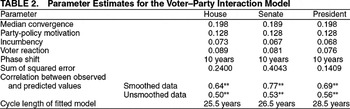
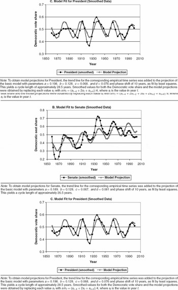
We fit the projections of the basic model described in the previous section separately to the empirical time-series for House, Senate, and president. Smoothed values are used for both empirical data and model projections.Footnote 14 Note first that any set of values of the parameters α, β, γ, δ, and the phase shift determines a time series using those parameters and generated by model equations 1–4—just as a set of regression parameters determines a regression equation and associated predicted values for all observations in the data set. In order to choose model parameter estimates to minimize the sum of least-square errors (between a theoretically projected time series and the empirical time series), we used an iterative method. In succession, each parameter estimate was selected by a search procedure to generate the smallest sum of squared error for that parameter, and the procedure was repeated until no change was observed in the estimated parameters to three decimal places. Estimated model parameters are presented in Table 2.
Parameter Estimates for the Voter–Party Interaction Model

Note: The symbol (**) indicates that the correlation between model prediction and the empirical data is significantly positive at the 0.01 level.
Based on these fits, cycle lengths were estimated to be approximately 25.5 years for the House, 26.5 years for the Senate, and 28.5 years for the president. The substantive message from these estimates is that fairly regular cycles occur for the House, Senate, and the president for which the cycle lengths are approximately the same. Furthermore the peaks and valleys of all three time series occur at approximately the same time.Footnote 15 The usual R-squared statistic for the proportion of variance explained is not available for assessing model fit (because the relevant sums of squares are not additive). Instead, we use as our measure of model fit the correlation between the observed values and the values predicted by the model. (In a linear regression this statistic is, when squared, the familiar R-squared.) As indicated in Table 2, this measure of model fit (for smoothed and detrended data) is 0.64, 0.77, and 0.69 for the House, Senate, and president, respectively, suggesting that the evidence for cycling for the presidential series is comparable to that for Congress. All three correlations (and those specified below) are significantly positive at the 0.01 level.
Alternatively, fitting the model with no smoothing of either data or model projections yields parameter estimates that differ from those obtained with smoothing at most by 0.006 and estimates of cycle lengths that differ at most by 0.5 years. As expected, without smoothing, the sums of squared errors of the fitted models are substantially larger, whereas the correlations between observed and predicted values are smaller. The correlations, however, are comparable in size among the presidential and Congressional series (see Table 2), just as they are for smoothed data.
An alternative model that features—in addition to the model elements above and unsmoothed data—an off-year-election effect and a coattail effect in presidential years also leads to similar parameter estimates as well as similar estimates for the cycling period. Plots showing the model fits and parameter estimates for all these model variations are available on our Web site (http://course.wilkes.edu/merrill/).
Visually, the model projections and smoothed House data, which are plotted in Figure 4A, show a remarkably close fit until about 1970, after which the patterns diverge somewhat. Particularly apparent is an unsurprising aberration from the projected pattern in the period immediately following Watergate. The fit for the smoothed Senate (Figure 4B) is also strong until 1970, whereas the post-Watergate perturbation is somewhat muted compared to that for the House. The fit for presidential elections (Figure 4C) is generally good throughout the 150-year period, with the model projection returning to the empirical pattern following the Watergate blip.
Model Fit to Congressional and Presidential Time Series

Comparative Statics
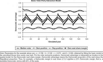
Figure 5 plots the Democratic margin, the median voter location, and the positions of both parties on the same graph, using the parameter estimates from the model fit to House data for illustration. The plot shows obvious, regular cycling for the partisan advantage in vote/seat share, with a cycle length—as indicated above—in the vicinity of 25 years. Note that the partisan share tracks the location of the median voter, which reflects voter preference, but with a lag such that a party retains majority status for 4 to 6 years after the median voter has crossed to the other side of the scale, suggesting that voter mood may be a leading indicator of partisan dominance. The ideological positions of the parties lag similarly behind the tides of the median voter.
Democratic Margin in Seat Share and Related Variables in the Voter–Party Interaction Model

We find that cycle length increases as either the median convergence parameter or the in-party advantage parameter increases, but decreases as either the party policy-motivation parameter or the voter reaction parameter increases. To see why cycle length increases as the median convergence parameter α increases, note that as a party moves more rapidly toward the median voter, it enhances its probability of maintaining majority status, hence lengthening the cycle. As we might expect, the cycle length also increases in the presence of the in-party advantage, embodied in the parameter γ.Footnote 16 Without any such incumbency advantage, no cycling occurs. With an in-party coefficient of γ = 0.04, the cycle length is about 12–14 years; for γ = 0.08, the cycle length lengthens to about 28 years, and for γ = 0.12, to about 48 years.
To account for shorter cycle lengths as a consequence of increasing the party policy-motivation parameter β, note that as the winning party pulls back more rapidly toward its preferred position, it erodes its majority status, thus shortening the cycle length. Likewise, as the voter reaction parameter δ increases, the median voter moves more strongly away from the party in power, thus truncating the latter's period of ascendancy. If β = 0, that is, there is no party policy motivation, both parties move to the median. As long as β is not zero, however, parties balance their partisan preferences with the pull of the median voter and remain intermediate between the median voter and their preferred positions. If δ = 0, that is, there is no voter response to the location of the governing party, the parties remain fixed in position. If either β = 0 or δ = 0, no cycling occurs. Overall, the model suggests that in-party effects may play an important role in generating regular cycles, although to do so, they must act in concert with other factors, such as the policy motivation of parties and interactive forces between parties and voters.
VARIATION OF DATA HANDLING AND MODEL ASSUMPTIONS
Effects of Minor Party Vote Share
Unfortunately, the partisan division of the popular vote for president is contaminated by a number of factors, including the presence of significant third-party (and in some cases fourth party) candidates in many of the elections, most notably the elections of 1860 (which featured two major Democratic candidates, Stephen A. Douglas and John C. Breckinridge as well as Whig candidate John Bell) and 1912 (in which Progressive nominee Theodore Roosevelt finished ahead of the Republican nominee William H. Taft). There seems to be no completely satisfactory way to handle these effects. In the basic model we have taken the simple approach of dividing the popular vote received by the leading Democratic nominee by the total popular vote received by that candidate and by the leading Republican nominee. An alternative presidential time series was constructed consisting of the Democratic proportion of the total vote in each election (the vote of the two major Democratic candidates was combined in 1860). Estimated cycle length based on this time series is about 25.5 years, essentially the same as that estimated from the two-party time series reported in Table 1B; the p-values for the statistical tests for the time series based on proportion of total vote are almost identical to those based on the two-party vote (p = 0.04 for Bartlett's test and p = 0.35 for Fisher's Kappa). Which of these approaches better reflects Democratic strength depends on the political leanings of the minor parties. The similarity, however, between the statistical inferences in these two approaches lends robustness to our findings. We prefer to focus on the two-party time series because it highlights the interplay between the two major parties over the last century and a half.
Other factors affecting the national popular vote include the greatly reduced turnout in most Southern states during much of the period before the mid-twentieth century—not to mention the complete absence of the eleven states of the Confederacy during the Civil War—and differential rules for the franchise across states. The time series for the Senate is affected by another factor—the fact that Senators were selected by state legislatures before the Seventeenth Amendment to the Constitution was ratified in 1913. Since, however, the time series seem relatively consistent over institutions and there does not appear to be a break in the Senatorial time series after 1913, we do not suspect that the uncertainties mentioned above have a major affect on our analysis.
Stochastic Assumptions
As another alternative, we expand our basic model by replacing deterministic assumptions with stochastic ones. In particular, we assume that there are random perturbations in both the location of the median voter and in the Democratic vote share. First, it is reasonable to presume that the voter distribution (and hence the location of the median voter) is affected not only by implemented policies but also by a myriad of other factors that cannot be estimated by either politicians or researchers and are best modeled as random variables. Similarly, the vote share of each party is subject to perturbations—due to such factors as valence characteristics of its candidates and changes in its national image—that cannot be predicted in advance.
We performed a computer simulation in which we perturb the location of the median voter and the (Democratic) vote share by normal variates each with mean zero and with standard deviations denoted by σM and σE, respectively. Implementation of the resulting stochastic model yields plots such as that in Figure W3 on the authors' Web site (http://course.wilkes.edu/merrill/), where we have used the same estimates a = 0.198, b= 0.128, c= 0.073, and d= 0.089 (for the first four parameters α, β, γ, and δ, respectively) as in the deterministic model fit to the House time series, and the stochastic parameters: σM = 0.025, and σE = 0.025. The vote-share trajectory now more closely resembles the globally regular but locally choppy pattern observed for the U.S. House. There is a rough cycle length of about 30 years. Cycles are partly obscured, as they are in real elections, but still apparent.
Alternative Assumptions Suggested by Empirical Studies
Empirical studies of voter–party interaction shed light on what model assumptions may be most appropriate. In particular, we may test the robustness of the model by considering alternative assumptions. Fowler and Smirnov (Reference Fowler and Smirnov2007; see also Fowler Reference Fowler2005; Smirnov and Fowler Reference Fowler and Smirnov2007)—speaking in modern terms—find that both the winning and losing parties in American politics become more liberal when the Democrats win, more conservative when the Republicans win, and the size of the change in ideology is increasing in the size of the margin of victory. In our model, policy-seeking parties/candidates face a tradeoff between advocating and implementing more extreme policies that they may prefer and more moderate policies that may attract the median voter, but when a party first wins (because the median voter has moved its way), both winners and losers move in the direction of the winning party as in the Fowler–Smirnov model, but in later victories both parties reverse direction away from the winning party and the size of this movement does not increase with the margin of victory.
Accordingly, to model the Fowler–Smirnov results, we maintain the same parameters for the winning party but replace the party policy-motivation parameter β with half its value for the losing party. Cycles occur as they did in the base model, but they are substantially shorter, 16 years in length. Both parties move in the direction of the winning party in nearly every election and the size of that movement is closely correlated with the size of the victory, as expected in the Fowler–Smirnov model.
Overall, we draw several conclusions from our sensitivity analysis. The existence of cycling appears relatively robust to model assumptions, at least those that we have investigated. The length of the cycles, however, is not robust either to variation of modeling assumptions or to variation of parameter values. Thus, the simulation results suggest strongly that, although cycling is likely and the duration of each cycle may be substantial in length, it is not feasible given the present state of our modeling technology to forecast the exact length of the cycles.
CONCLUSION
Statistical evidence suggests that, broadly speaking, the partisan seat share of the Democratic and Republican parties in the U.S. Congress and their vote share for president has not varied randomly over time but rather has oscillated back and forth in a fairly regular pattern for the past 160 years. The statistical analysis suggests that the period of that oscillation—the time duration required for the state of the system to return to a given state—is approximately 25 to 30 years. Thus, for example, when a party first attains a majority in Congress and/or the presidency, it is likely to stay in power—first rising then falling in seat share—for 12 to 15 years before ceding majority status to the other party, which then enjoys a similar predominance for 12 to 15 years. Superimposed on this general pattern are idiosyncratic perturbations that partially disrupt the overall pattern, so that the actual period of dominance may vary from the expected and may be interspersed with periods of minority or opposition status. During portions of American history, furthermore, one party of the other has been generally stronger, so that the duration of its majority status may have exceeded 12 to 15 years, whereas that of its opponent has been shorter.
To better understand the 12–15 half-period we uncovered, we have impressionistically reviewed the historical record to get a more intuitive feel about the specific political events linked to rise and fall in party strength and to issues of timing. But we have deliberately eschewed adding such a discussion to this paper since it takes us into historical issues beyond the scope of this paper and outside the specific expertise of the authors. Suffice it to note that our results are not incompatible with traditional accounts of the period from the 1860s through the 1970s and perhaps beyond—including the Schlesingers' cycles of liberalism and conservatism over much of the twentieth century—but offer a much more nuanced picture, involving ebbs and flows and not just critical elections.
In an attempt to explain this regular cycling, we have developed a voter-party interaction model. The predictions of the model depend on tensions of two types, one involving parties and the other involving voters. First there is the centrifugal–centripetal tension between the parties' preferred policies on the one hand and their attraction to the median voter on the other. Which of these attractions has the greater influence is reflected in the relative size of the party-policy-motivation parameter and the median convergence parameter. Second, voters exhibit a tension between a tendency to value incumbency and in-party status—effects that tends to lengthen cycles—and a countervailing inclination to move away from the policies of the party in power—which tends to shorten cycles. The relative strength of these two opposing forces is related to the relative size of the incumbency advantage parameter and the voter reaction parameter.
In sum, although we are in agreement with much of Mayhew's (2002) critique of the traditional realignment literature, that does not mean that we should “throw away the baby with the bathwater” and reject clear evidence for ebb and flow in partisan tides of the sort presented in this paper. Moreover, we need to model the reasons for such ebb and flow, and we offer the second part of this essay as a useful beginning in that regard. Our evidence suggests that realignments should not be viewed only as phenomena of punctuated equilibrium. Instead, we emphasize the long-term and incremental ebb and fall of national party support patterns. Moreover, our statistical evidence suggests a shorter cycle of rise and fall than was suggested by some earlier realignment theorists and allows for the fact that some such swings may not involve changes in party control but rather diminutions in the dominance of the larger party (see also Sprague Reference Sprague1981).
But we would emphasize that the evidence in this paper bears only on the first of the five notions of realignment that we have previously described, namely, change in party dominance. The equivalence (or nonequivalence) of the various other ways of thinking about realignment needs to be a matter for empirical investigation. While we have shown clear evidence of partisan tides that are at least somewhat durable and have a cyclic form, we are certainly not espousing the kind of “strong” version of realignment theory rebutted by Mayhew (2002)—one which defines realignments in terms of dramatic and long-lasting changes in party ascendancy that change all aspects of previous political coalitions (sociodemographic voting patterns, attitudinal, cleavage structure, regional support base), and affect all levels of government.
We note in passing, however, that by 2000 at the latest, there was solid evidence that a realignment away from the Civil War and New Deal voting alignments had occurred in terms of various dimensions claimed as important by realignment theorists. In particular, while there still are some substantial continuities in the demographic support base of the two parties, the almost total flip-flop in the regional bases of party support is impossible to miss (see, e.g., Schofield Reference Schofield2006 for U.S. presidential contests, or Brunell and Grofman Reference Brunell and Grofman1998 for the U.S. Senate).
However, the one-dimensional model that we offer should be seen as only one possible approach, with our chief claim being that, even if we do not complicate our story with more than one dimension, we can still get cyclic patterns. Multidimensional models of political competition, which focus on the introduction of new issues (see Riker Reference Riker1982; Poole and Rosenthal Reference Poole and Rosenthal1997) and/or the attempts of one party to make inroads into the other party's supporters (e.g., Schofield Reference Schofield2006) can also lead to cycles of political dominance. Discussion of such models would, however, takes us into matters well beyond the scope of this essay.
The preliminary model we have offered in this paper predicts a pattern of oscillation in party strengths, but not an unbounded one—opposing tensions exist in the model that maintain stability in the output in a negative feedback loop. As we have shown, such a model appears to fit the broad outlines of American partisan politics for the last century and a half.
 . Replacing the probability 0.5 with the actual proportions for the historical period changes the p-values of the test by less than 0.001 except for president (from p = 0.25 to p = 0.26). The test we use is slightly different from the runs test that assumes a priori the total number of D's and the total number of R's—quantities that are not known in our application.



Comments
No Comments have been published for this article.