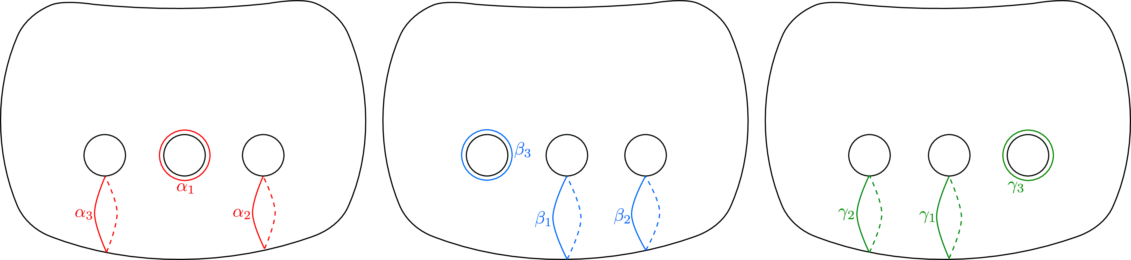


1. Introduction
A trisection, which was introduced by Gay and Kirby [
Reference Gay and Kirby5
], is roughly a decomposition of a closed oriented smooth 4-manifold into three 4-dimensional 1-handlebodies, namely, the union of a 0-handle and 1-handles. A trisection is a 4-dimensional analogue of a Heegaard splitting, a well known decomposition of a 3-manifold into two 3-dimensional 1-handlebodies. Just as the decomposition of a Heegaard splitting is described by a Heegaard diagram, the decomposition of a trisection is described by a trisection diagram. A trisection diagram is a 4-tuple which consists of a closed oriented surface appearing as the triple intersection of components of the decomposition and three families of simple closed curves
 $\alpha$
,
 $\beta$
and
 $\gamma$
in the surface. There is a one-to-one correspondence between trisections and trisection diagrams under an appropriate equivalence relation. A trisection diagram recovers a handle decomposition of the 4-manifold by taking the product of a 2-dimensional disk to the surface and attaching 2-handles along the
 $\alpha$
,
 $\beta$
and
 $\gamma$
curves with the surface framings.
It is shown as a corollary from the existence and uniqueness of trisections up to stabilisation that two closed 4-manifolds are diffeomorphic if and only if two corresponding trisection diagrams are related by surface diffeomorphisms, handle slides among the same family curves and stabilisations. However, given two trisection diagrams of the same 4-manifold with the same type (see Definition 2·2 for the type of a trisection diagram), it is generally difficult to decide whether stabilisations are necessary or not. Here, let us recall examples where stabilisations are required and where they are not. As an example of the former case, Islambouli [
Reference Islambouli9
] showed that there exist spun Seifert fibered spaces that admit non-isotopic trisections with the same type. Namely, trisection diagrams corresponding to these 4-manifolds cannot be related to each other without stabilisations. As an example of the latter case, it is easy to check that the two (2,0)-trisection diagrams of
 $\mathbb{C}P^2 \# \overline{\mathbb{C}P^2}$
and
 $S^2 \tilde{\times} S^2$
, the non-trivial sphere bundle over the sphere, depicted in [
Reference Gay and Kirby5
], are related without stabilisations. With respect to
 $S^4$
, it is conjectured, called the 4-dimensional Waldhausen conjecture, that each trisection of
 $S^4$
is isotopic to the genus-0 trisection or its stabilisation [
Reference Meier, Schirmer and Zupan15
]. In terms of trisection diagrams, the 4-dimensional Waldhausen conjecture asserts that each trisection diagram
 $\mathcal{D}$
of
 $S^4$
is related to the stabilisation of the genus-0 trisection diagram, whose type is the same as the type of
 $\mathcal{D}$
, without stabilisations. Actually, there is some supporting evidence of the conjecture (for example, [
Reference Isoshima10, Reference Meier, Schirmer and Zupan15
]. However, this conjecture is believed to be false at present by [
Reference Meier, Schirmer and Zupan15
], and there are some potential counterexamples. In this paper, we explore one family of potential counterexamples coming from trisections of Gluck twisted 4-manifolds that are diffeomorphic to
 $S^4$
.
The Gluck twist is a cutting and pasting operation on a 2-knot. Let X be a closed 4-manifold and K be a 2-knot in X with normal Euler number 0. Then, the Gluck twisted 4-manifold
 $\Sigma_K(X) = X-{\rm int}(\nu(K)) \cup_{\tau} S^2 \times D^2$
, where
 $\tau$
is the non-trivial self-diffeomorphism of
 $S^2 \times S^1$
defined by
 $\tau(z,e^{i\theta})=(ze^{i\theta}, e^{i\theta})$
, and
 $\nu(K)$
is a tubular neighbourhood of K in X. If
 $X=S^4$
, the Gluck twisted 4-manifold on any 2-knot is a homotopy 4-sphere [
Reference Gluck7
], and hence homeomorphic to
 $S^4$
by Freedman’s theorem [
Reference Freedman4
]. Moreover, it is well known that
 $\Sigma_K(S^4)$
is diffeomorphic to
 $S^4$
if K is a spun 2-knot or twist-spun 2-knot [
Reference Gluck7, Reference Gordon8
]. Thus, a corresponding trisection diagram and the stabilisation of the genus-0 trisection diagram are related by the three operations including stabilisations. However, it is not known if the resulting trisection diagram can be destabilised some number of times to get the genus-0 trisection diagram, or if stabilisations are required. Then, Gay and Meier asked the following question:
Question 1·1 ([
Reference Gay and Meier6
]). Let
 $\mathcal{K}$
be the spin or the twist-spin of a non-trivial knot K in
 $S^3$
. Is a trisection diagram of
 $\Sigma_{\mathcal{K}}({S^4})$
constructed from a doubly-pointed Heegaard diagram of K by combining some methods ever standard?
Note that we say that a trisection diagram of a 4-manifold that is diffeomorphic to
 $S^4$
is standard if it is the stabilisation of the genus-0 trisection diagram after surface diffeomorphisms and handle slides.
The first answer to Question 1·1 was obtained in [
Reference Isoshima and Ogawa11
, theorem 1·1], in which the author and Ogawa showed that in Question 1·1, if we take the trefoil knot as the 1-knot K and take Figure 3 as its doubly-pointed Heegaard diagram, then the trisection diagram of
 $\Sigma_{\mathcal{K}}({S^4})$
in Question 1·1 is standard.
Let
 $\mathcal{D}_p$
be the trisection diagram of
 $\Sigma_{S(T(p+1,p))}({S^4})$
in Question 1·1 obtained by taking the
 $(p+1,p)$
-torus knot
 $T(p+1,p)$
as the 1-knot K and taking Figure 3 as its doubly-pointed Heegaard diagram, where
 $S(T(p+1,p))$
is the spun
 $(p+1,p)$
-torus knot. The trisection diagram
 $\mathcal{D}_p$
is shown explicitly in Figure 15. In this paper, we show the following main theorem.
Theorem (Theorem 4·1). The trisection diagram
 $\mathcal{D}_p$
(
 $p \ge 2$
) is standard.
Note that [
Reference Isoshima and Ogawa11
, theorem 1·1] corresponds to the case of
 $p=2$
in the main theorem. The proof of the theorem requires a large number of Dehn twists and handle slides, as well as an inductive argument we call the seesaw lemma (Lemma 4·6).
Organisations. We briefly review preliminaries, specifically (relative) trisections of 4-manifolds (with boundary) and doubly pointed Heegaard/trisection diagrams in Section 2. In Section 3, we construct the trisection diagram in the question for the spun
 $(p+1,p)$
-torus knot explicitly by the methods mentioned in the question. Then we prove the main theorem in Section 4. We have further remarks in Section 5.
2. Preliminaries
In this section, we review notions used in Section 3 and 4. In this paper, unless otherwise stated, any 4-manifold is compact, connected, oriented and smooth, and any surface-knot is a connected, closed surface smoothly embedded in a 4-manifold.
2·1. Trisections and relative trisections
In this subsection, we recall (relative) trisections of 4-manifolds (with boundary).
Definition 2·1. Let X be a closed 4-manifold. A
 $(g;\;k_1,k_2,k_3)$
-trisection of X is a 3-tuple
 $(X_1,X_2,X_3)$
satisfying the following conditions:
-
(i)
 $X=X_1 \cup X_2 \cup X_3$
;
-
(ii) for each
$i=1,2,3$
,
$X_i \cong \natural_{k_i} S^1 \times D^3$
; -
(iii) for each
$i=1,2,3$
,
$X_i \cap X_j \cong \natural_{g} S^1 \times D^2$
; -
(iv)
$X_1 \cap X_2 \cap X_3 \cong \#_{g} S^1 \times S^1 = \Sigma_g$
.


Note that g and
 $k_i$
are non-negative integers with
 $k_i \le g$
for each i. Let
 $H_{\alpha} = X_3 \cap X_1$
,
 $H_{\beta} = X_1 \cap X_2$
and
 $H_{\gamma} = X_2 \cap X_3$
. The union
 $H_{\alpha} \cup H_{\beta} \cup H_{\gamma}$
is called the spine of the trisection. A trisection is uniquely determined by its spine. The 4-tuple of non-negative integers
 $(g;\;k_1,k_2,k_3)$
is called the type of the trisection. Note that if
 $k_1=k_2=k_3$
, the trisection is said to be balanced, and the type is denoted by (g,k) for short, where
 $k=k_i$
(
 $i=1,2,3$
). Each
 $X_i$
is called a sector.
The decomposition of a trisection is described by a trisection diagram.
Definition 2·2. A 4-tuple
 $(\Sigma_g,\alpha,\beta,\gamma)$
is called a
 $(g;\;k_1,k_2,k_3)$
-trisection diagram if the following holds:
-
(i)
$(\Sigma_g,\alpha,\beta)$
is a Heegaard diagram of
$\#_{k_1}S^1 \times S^2$
; -
(ii)
$(\Sigma_g,\beta,\gamma)$
is a Heegaard diagram of
$\#_{k_2}S^1 \times S^2$
; -
(iii)
$(\Sigma_g,\gamma,\alpha)$
is a Heegaard diagram of
$\#_{k_3}S^1 \times S^2$
.


Similar to the type of a trisection, the 4-tuple of non-negative integers
 $(g;\;k_1,k_2,k_3)$
is called the type of the trisection diagram.
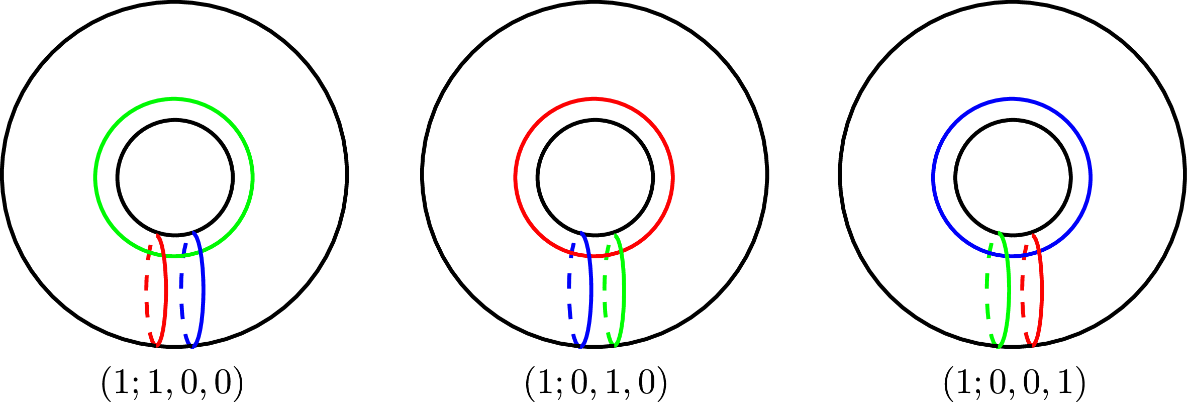
Definition 2·3. A stabilisation of a trisection diagram is the connected-sum of the trisection diagram and the genus 1 trisection diagram of
 $S^4$
depicted in Figure 1. The reverse operation is called a destabilisation.
Note that this (de)stabilisation is the unbalanced one.
Every 4-manifold admits a trisection, and any two trisections of the same 4-manifold are isotopic after performing some number of stabilisations [ Reference Gay and Kirby5 ]. As a corollary, it is known that any two closed 4-manifolds are diffeomorphic if and only if two corresponding trisection diagrams are related by surface diffeomorphisms, handle slides among the same family curves and balanced stabilisations.
Let X and Y be diffeomorphic closed 4-manifolds. Two trisections
 $(X_1, X_2, X_3)$
of X and
 $(Y_1,Y_2,Y_3)$
of Y are diffeomorphic if there exists a diffeomorphism
 $h \colon X \to Y$
such that
 $h(X_i)=Y_i$
for each
 $i=1,2,3$
. Two trisections
 $(X_1, X_2, X_3)$
and
 $(Y_1,Y_2,Y_3)$
of a 4-manifold Z are isotopic if there exists an isotopy
 $h_t \colon Z \to Z$
such that
 $h_0=id_{Z}$
and
 $h_1(X_i)=Y_i$
for each
 $i=1,2,3$
. Two trisections are diffeomorphic if and only if two corresponding trisection diagrams are related without stabilisations. It is conjectured that each trisection of
 $S^4$
is isotopic to the genus-0 trisection or its stabilisation [
Reference Meier, Schirmer and Zupan15
]. A counterexample of this conjecture may be given via trisection diagrams of a 4-manifold diffeomorphic to
 $S^4$
since any two isotopic trisections are diffeomorphic.
The genus 1 trisection diagrams of
 $S^4$
.

Trisections of 4-manifolds with boundary are called relative trisections [
Reference Castro1
]. We recall them here. For the disk
 $D=\{re^{i\theta} \mid r\in [0, 1] , -\pi/3\leq \theta \leq \pi / 3 \} \subset \mathbb{C}$
, let
 \[ {} \partial ^{-} D = \{re^{\pi/3} \in \partial D \mid r\in [0, 1]\},\]
 \[ {}\partial^{0} D = \{e^{i\theta}\in \partial D\}\; \text{and}\]
 \[ {} \partial^{+} D = \{re^{-\pi/3} \in \partial D \mid r\in [0, 1]\}.\]
Then,
 $\partial{D}=\partial ^{-} D \cup \partial^{0} D \cup \partial^{+} D$
. For a genus p surface P with b boundary components,
 $U\;:\!=\;P\times D$
is diffeomorphic to
 $\natural_{2p+b-1} S^1\times B^3$
. Furthermore, its boundary is decomposed into
 $\partial ^0 U = (P\times \partial ^{0} D) \cup (\partial P \times D)$
and
 $\partial ^{\pm} U = P\times \partial^{\pm} D$
. Let
 $V_n$
be
 $\natural_n (S^1\times B^3)$
and
 $\partial V_n = H_s^{-}\cup H_{s}^{+}$
a genus
 $n+s$
Heegaard splitting of
 $\partial V_n$
.
Let
 $s=g-k+p+b-1$
and
 $n=k-2p-b+1$
. Then, we have
 $Z_k\cong U\natural V_n\cong \natural_k S^1\times B^3$
. Note that
 \[ {}\partial Z_k = Y^{+}_{g, k ;\; p, b}\cup Y^{0}_{g, k ;\; p, b}\cup Y^{-}_{g, k ;\; p, b},\]
where
 $Y^{\pm}_{g, k ;\; p, b}=\partial ^{\pm} U\natural H_{s}^{\pm}$
and
 $Y^{0}_{g, k ;\; p, b}= \partial ^0 U$
. Under the above settings, we define relative trisections as follows.
Definition 2·4. Let W be a 4-manifold with connected boundary. A decomposition
 $W=W_1\cup W_2\cup W_3$
of W is called a
 $(g, k;\; p, b)$
-relative trisection of W if the followings hold:
-
(i)
$W_i\cong Z_k$
for
$i=1, 2, 3$
; -
(ii)
$W_i\cap W_{i+1} \cong Y^{+}_{g, k ;\; p, b}$
and
$W_i\cap W_{i-1}\cong Y^{-}_{g, k ;\; p, b}$
for
$i=1, 2, 3$
.


It follows from these conditions that
 $W_1\cap W_2\cap W_3$
is a genus g surface with b boundary components.
As in the closed case, relative trisection diagrams can be defined for relative trisections [ Reference Castro, Gay and Pinzón-Caicedo2 ].
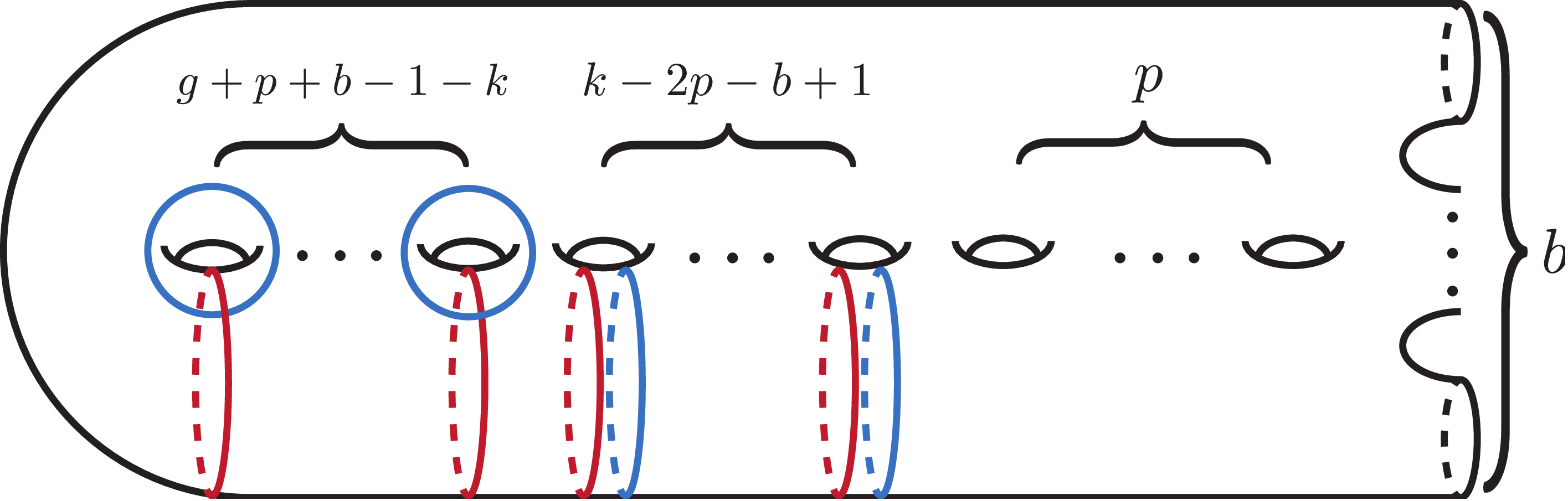
The standard diagram for relative trisection diagrams.

Definition 2·5. For a genus g surface
 $\Sigma$
with b boundary components and three sets of
 $g-p$
simple closed curves
 $\alpha$
,
 $\beta$
and
 $\gamma$
on
 $\Sigma$
, a
 $(g, k;\; p, b)$
- relative trisection diagram is a 4-tuple
 $(\Sigma;\; \alpha, \beta, \gamma)$
such that each of
 $(\Sigma;\; \alpha, \beta)$
,
 $(\Sigma;\; \beta, \gamma)$
and
 $(\Sigma;\; \gamma,\alpha)$
is related to the diagram depicted in Figure 2 by surface diffeomorphisms and handle slides.
Arced relative trisection diagrams, which are needed when we consider gluing two relative trisection diagrams, are defined for relative trisection diagrams.
Definition 2·6. Let
 $(\Sigma,\alpha,\beta,\gamma)$
be a
 $(g,k;\;p,b)$
-relative trisection diagram, and
 $\mathfrak{a}$
,
 $\mathfrak{b}$
and
 $\mathfrak{c}$
collections of 2p properly embedded arcs in
 $\Sigma$
. Suppose that the arcs
 $\mathfrak{a}$
(resp.
 $\mathfrak{b}$
and
 $\mathfrak{c}$
) are disjoint from
 $\alpha$
(resp.
 $\beta$
and
 $\gamma$
). A tuple
 $(\Sigma,\alpha,\beta,\gamma,\mathfrak{a},\mathfrak{b},\mathfrak{c})$
is called an arced relative trisection diagram if the following conditions hold:
-
(i) cutting
$\Sigma_\alpha$
(resp.
$\Sigma_\beta$
,
$\Sigma_\gamma$
) along
$\mathfrak{a}$
(resp.
$\mathfrak{b}$
,
$\mathfrak{c}$
) yields a disk, where
$\Sigma_x$
is a surface obtained by surgering
$\Sigma$
along x for
$x \in \{\alpha, \beta, \gamma\}$
; -
(ii) by handle slides,
$(\Sigma,\alpha,\beta,\mathfrak{a},\mathfrak{b})$
is related to some
$(\Sigma,\alpha^{'},\beta^{'},\mathfrak{a}^{'},\mathfrak{b}^{'})$
such that
$(\Sigma,\alpha^{'},\beta^{'})$
is related to the diagram shown in Figure 2 and
$\mathfrak{a}^{'} = \mathfrak{b}^{'}$
; -
(iii) by handle slides,
$(\Sigma,\beta,\gamma,\mathfrak{b},\mathfrak{c})$
is related to some
$(\Sigma,\beta^{'},\gamma^{'},\mathfrak{b}^{'},\mathfrak{c}^{'})$
such that
$(\Sigma,\beta^{'},\gamma^{'})$
is related to the diagram shown in Figure 2 and
$\mathfrak{b}^{'} = \mathfrak{c}^{'}$
.


An algorithm for drawing the arcs is developed in [ Reference Castro, Gay and Pinzón-Caicedo2 , theorem 5].
Theorem 2·7 ([
Reference Castro, Gay and Pinzón-Caicedo2
, theorem 5]). Let
 $(\Sigma,\alpha,\beta,\gamma)$
be a relative trisection diagram and
 $\Sigma_\alpha$
the surface obtained by surgering
 $\Sigma$
along
 $\alpha$
and
 $\phi \colon \Sigma \backslash \alpha \to \Sigma_\alpha$
an associated embedding. Then, collections
 $\mathfrak{a}$
,
 $\mathfrak{b}$
and
 $\mathfrak{c}$
of arcs in
 $\Sigma$
are obtained by taking the procedure below in order.
-
(i) There exists a collection of properly embedded arcs
$\delta$
in
$\Sigma_\alpha$
such that cutting
$\Sigma_\alpha$
along
$\delta$
produces the disk. Then, let
$\mathfrak{a}$
denote a collection of properly embedded arcs in
$\Sigma-\alpha$
such that
$\delta$
is isotopic to
$\phi(\mathfrak{a})$
in
$\Sigma_\alpha$
. -
(ii) A collection of arcs in
$\Sigma$
that is disjoint from
$\beta$
can be obtained by sliding a copy of
$\mathfrak{a}$
over
$\alpha$
. Then, let
$\mathfrak{b}$
denote the collection of arcs. Note that in this operation, sliding a
$\beta$
curve over other
$\beta$
curves can be performed if necessary. -
(iii) A collection of arcs in
$\Sigma$
that is disjoint from
$\gamma$
can be obtained by sliding a copy of
$\mathfrak{b}$
over
$\beta$
. Then, let
$\mathfrak{c}$
denote the collection of arcs. Note that in this operation, sliding a
$\gamma$
curve over other
$\gamma$
curves can be performed if necessary.


2·2. Doubly pointed Heegaard/trisection diagrams
We first recall bridge decompositions of classical knots in 3-manifolds.
Definition 2·8. Let H be a 3-dimensional 1-handlebody and
 $\tau=\{\tau_i\}$
a collection of arcs properly embedded in H. We say that
 $\tau$
is trivial if
 $\tau_i$
can be isotoped into
 $\partial{H}$
for each i, or equivalently, there exists a collection
 $\Delta=\{\Delta_i\}$
of disks in H with
 $\Delta_i \cap \Delta_j =\emptyset$
such that
 $\partial{\Delta_i} = \tau_i \cup \tau_i^{'}$
for some arc
 $\tau_i^{'} \subset \partial{H}$
. We call
 $\tau$
,
 $\Delta$
and
 $\tau_i^{'}$
trivial tangles, bridge disks and a shadow of
 $\tau_i$
, respectively.
Let
 $M=H_1 \cup H_2$
be a Heegaard splitting of a closed 3-manifold M and K a knot in M. For a positive integer b, a decomposition
 $(M,K)=(H_1,H_1\cap K) \cup (H_2,H_2\cap K)$
of (M,K) is called a b-bridge decomposition if
 $H_i \cap K$
consists of b trivial arcs for
 $i=1,2$
. It is known that every knot admits a 1-bridge decomposition by meridional stabilisations. A knot admitting a 1-bridge decomposition can be described by a doubly pointed Heegaard diagram which is a Heegaard diagram
 $(\Sigma,\alpha,\beta,z,w)$
of the 3-manifold with two base points z and w on
 $\Sigma$
that are disjoint from
 $\alpha$
and
 $\beta$
. The union of two arcs connecting the two base points in each handlebody of the Heegaard splitting describes the knot, and a knot can be determined uniquely by the two base points. For more details, see [
Reference Ording19
] for example.
Similar to bridge decompositions of classical knots in 3-manifolds, bridge trisections of surface knots in 4-manifolds are introduced in [ Reference Meier and Zupan16, Reference Meier and Zupan17 ].
Definition 2·9. Let V be a 4-dimensional 1-handlebody and
 $\mathcal{D}$
a collection of disks properly embedded in V. We say that
 $\mathcal{D}$
is trivial if the disks of
 $\mathcal{D}$
can be simultaneously isotoped into
 $\partial{V}$
.
Definition 2·10. Let
 $X=X_1 \cup X_2 \cup X_3$
be a
 $(g;\;k_1,k_2,k_3)$
-trisection of a closed 4-manifold X, and S a surface-knot in X. A decomposition
 $(X,S) = (X_1,\mathcal{D}_1) \cup (X_2,\mathcal{D}_2) \cup (X_3,\mathcal{D}_3)$
is called a
 $(g;\;k_1,k_2,k_3;\;b;\;c_1,c_2,c_3)$
-bridge trisection of (X,S) if the following hold:
-
(i) for each
$i=1,2,3$
,
$\mathcal{D}_i$
is a collection of
$c_i$
trivial disks in
$X_i$
; -
(ii) for
$i \not= j$
, the intersection
$\mathcal{D}_i \cap \mathcal{D}_j$
forms b trivial tangles in
$X_i \cap X_j$
.


We say that S is in
 $(b;\;c_1,c_2,c_3)$
-bridge position with respect to the trisection
 $(X_1,X_2,X_3)$
if
 $(X,S) = (X_1,S \cap X_1) \cup (X_2,S \cap X_2) \cup (X_3,S \cap X_3)$
is a
 $(g;\;k_1,k_2,k_3;\;b;\;c_1,c_2,c_3)$
-bridge trisection. In particular, if
 $c_1=c_2=c_3$
, we simply say that S is in b-bridge position.
Definition 2·11. Let
 $(X,S)=(X_1,\mathcal{D}_1) \cup (X_2,\mathcal{D}_2) \cup (X_3,\mathcal{D}_3)$
be a bridge trisection. A 4-tuple
 $(\Sigma, (\alpha, \mathfrak{a}), (\beta, \mathfrak{b}), (\gamma, \mathfrak{c}))$
is called a shadow diagram if the 4-tuple
 $(\Sigma,\alpha,\beta,\gamma)$
is a trisection diagram of the trisection
 $(X_1,X_2,X_3)$
of X, and
 $\mathfrak{a}$
,
 $\mathfrak{b}$
and
 $\mathfrak{c}$
are shadows of
 $\mathcal{D}_1 \cap \mathcal{D}_2$
,
 $\mathcal{D}_2 \cap \mathcal{D}_3$
and
 $\mathcal{D}_3 \cap \mathcal{D}_1$
, respectively. In particular, if each of
 $\mathfrak{a}$
,
 $\mathfrak{b}$
and
 $\mathfrak{c}$
consists of one shadow of
 $\mathcal{D}_i \cap \mathcal{D}_j$
, the shadow diagram is called a doubly-pointed trisection diagram.
Similar to doubly-pointed Heegaard diagrams, for a trisection diagram
 $(\Sigma, \alpha, \beta, \gamma)$
, a doubly-pointed trisection diagram is often denoted by
 $(\Sigma, \alpha, \beta, \gamma, z, w)$
, where z and w are two base points on
 $\Sigma$
that are disjoint from
 $\alpha$
,
 $\beta$
and
 $\gamma$
. It is known that every 2-knot can be put in 1-bridge position by meridional stabilisations [
Reference Meier and Zupan16, Reference Meier and Zupan17
]. Namely, every 2-knot can be described by a doubly-pointed trisection diagram. The union of three arcs connecting the two base points in each sector of the trisection describes the 2-knot, and a 2-knot can be determined uniquely by the two base points. See [
Reference Meier and Zupan16, Reference Meier and Zupan17
] for more details.
3. Constructing trisection diagrams for Gluck twisting
In this section, we construct the trisection diagram (Lemma 3·3) in Question 1·1 for the spun
 $(p+1,p)$
-torus knot
 $S(T(p+1,p))$
, where
 $T(p+1,p)$
denotes the
 $(p+1,p)$
-torus knot. The construction is similar to the one in [
Reference Isoshima and Ogawa11
, section 3]. Note that
 $t_c$
denotes the right-handed Dehn twist along a simple closed curve c.
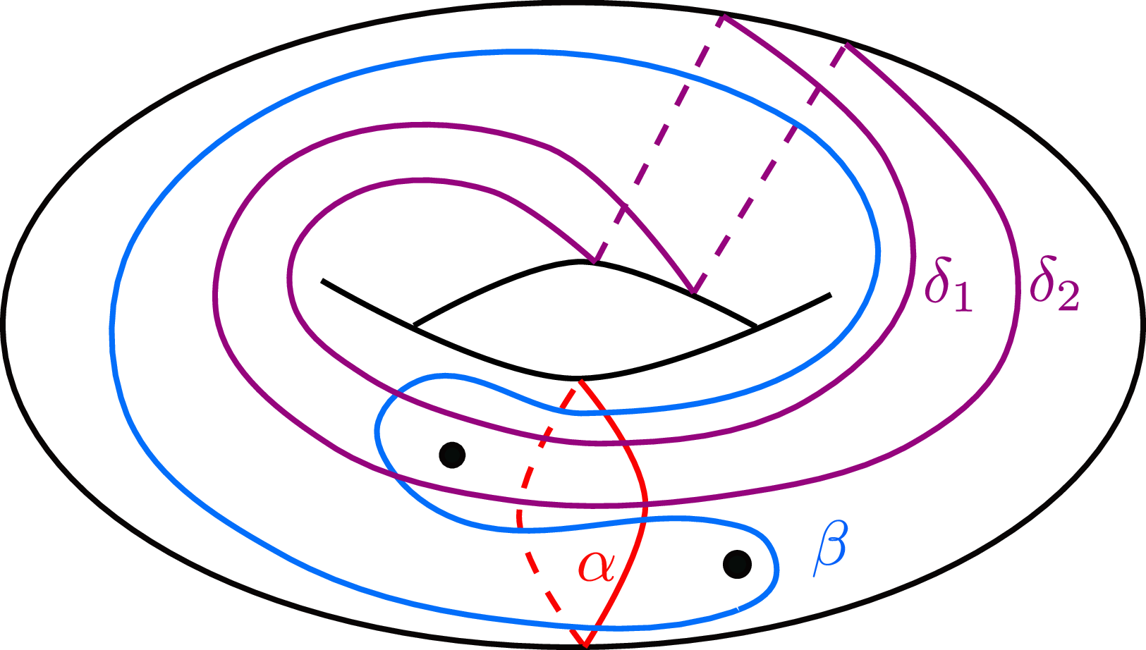
A doubly-pointed Heegaard diagram of
 $(S^3, T(3,2))$
and the curves
 $\delta_1$
and
 $\delta_2$
.

Lemma 3·1. Let
 $(\Sigma, \alpha, \beta, z, w)$
be a doubly-pointed Heegaard diagram of
 $(S^3, T(3,2))$
depicted in Figure 3. Then, for
 $p \ge 2$
,
 $(\Sigma, \alpha, t_{\delta_1}^{p-2}t_{\delta_2}^{-(p-2)}(\beta), z, w)$
is a doubly-pointed Heegaard diagram of
 $(S^3, T(p+1,p))$
, where
 $\delta_1$
and
 $\delta_2$
are the curves depicted in Figure 3.
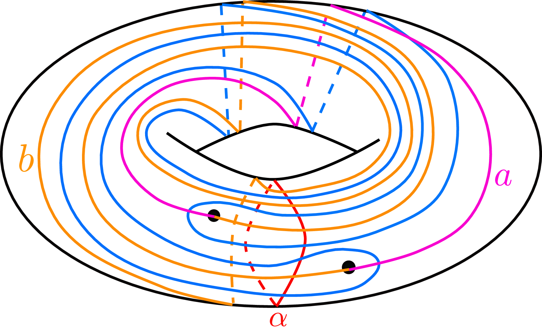
Proof. Figure 4 is the doubly-pointed Heegaard diagram
 $(\Sigma, \alpha, t_{\delta_1}^{p-2}t_{\delta_2}^{-(p-2)}(\beta), z, w)$
. Note that
 $(\Sigma, \alpha, t_{\delta_1}^{p-2}t_{\delta_2}^{-(p-2)}(\beta))$
is a Heegaard diagram of
 $S^3$
since
 $\delta_1$
and
 $\delta_2$
can be parallel in the Heegaard diagram. Then, arcs a and b for
 $\alpha$
and
 $t_{\delta_1}^{p-2}t_{\delta_2}^{-(p-2)}(\beta)$
, respectively, can be drawn as in Figure 4. The union
 $a \cup b$
describes the
 $(p+1,p)$
-torus knot
 $T(p+1,p)$
. This completes the proof.
Figure 5 is the doubly-pointed Heegaard diagram
 $(\Sigma, \alpha, t_{\delta_1}t_{\delta_2}^{-1}(\beta), z, w)$
of
 $(S^3, T(4,3))$
for example. Lemma 3·1 corresponds to [
Reference Isoshima and Ogawa11
, lemma 3·6] in the case of
 $(S^4, T(2n+1,2))$
.
The doubly-pointed Heegaard diagram
 $(\Sigma, \alpha, t_{\delta_1}^{p-2}t_{\delta_2}^{-(p-2)}(\beta), z, w)$
of
 $(S^3, T(p+1,p))$
and arcs a and b. The union
 $a \cup b$
describes
 $T(p+1,p)$
.

The doubly-pointed Heegaard diagram
 $(\Sigma, \alpha, t_{\delta_1}t_{\delta_2}^{-1}(\beta), z, w)$
of
 $(S^3, T(4,3))$
and arcs a and b. The union
 $a \cup b$
describes T(4,3).

An arced relative trisection diagram of
 $S^4-S(T(3,2))$
and the curves
 $\delta_1^{\beta}$
,
 $\delta_2^{\beta}$
,
 $\delta_1^{\gamma}$
and
 $\delta_2^{\gamma}$
. See also Figure 7 for visual clarity.

Lemma 3·2. Let
 $(\Sigma, \alpha, \beta, \gamma, a, b, c)$
be an arced relative trisection diagram of
 $S^4-S(T(3,2))$
depicted in Figure 6. Then, for
 $p \ge 2$
,
 $(\Sigma, \alpha', \beta', \gamma', a', b', c')$
is an arced relative trisection diagram of
 $S^4-S(T(p+1,p))$
, where:
-
(i)
$\alpha' = (t_{\delta_1^{\beta}}^{p-2}t_{\delta_2^{\beta}}^{-(p-2)}(\alpha_1), \alpha_2, \alpha_3)$
; -
(ii)
$\beta' = (t_{\delta_1^{\beta}}^{p-2}t_{\delta_2^{\beta}}^{-(p-2)}(\beta_1), \beta_2, \beta_3)$
; -
(iii)
$\gamma' = (t_{\delta_1^{\gamma}}^{p-2}t_{\delta_2^{\gamma}}^{-(p-2)}(\gamma_1), \gamma_2, \gamma_3)$
; -
(iv)
$a' = t_{\delta_1^{\beta}}^{p-2}t_{\delta_2^{\beta}}^{-(p-2)}(a)$
; -
(v)
$b' = t_{\delta_1^{\beta}}^{p-2}t_{\delta_2^{\beta}}^{-(p-2)}(b)$
; -
(vi)
$c' = t_{\delta_1^{\gamma}}^{p-2}t_{\delta_2^{\gamma}}^{-(p-2)}(c)$
;


and the curves
 $\delta_1^{\beta}$
,
 $\delta_2^{\beta}$
,
 $\delta_1^{\gamma}$
and
 $\delta_2^{\gamma}$
are the ones depicted in Figure 6.
Proof. By applying Meier’s spinning method [
Reference Meier14
] (see also [
Reference Isoshima and Ogawa11
, subsection 3·1]) to Lemma 3·1 and Figure 3, we have a doubly-pointed trisection diagram of
 $(S^4, S(T(p+1,p)))$
. See [
Reference Isoshima and Ogawa11
, figure 4 and lemma 3·7] in the case of
 $(S^4, S(T(2n+1,2)))$
. Then, by removing a neighbourhood of the base points (two black points z and w) of the doubly-pointed trisection diagram, we get a relative trisection diagram of
 $S^4-S(T(p+1,p))$
. See [
Reference Isoshima and Ogawa11
, figure 5 and lemma 3·8] in the case of
 $(S^4, S(T(2n+1,2)))$
. Lastly, by using an algorithm for drawing arcs of relative trisection diagrams [
Reference Castro, Gay and Pinzón-Caicedo2
] (see also [
Reference Isoshima and Ogawa11
, subsection 3·3]), we obtain an arced relative trisection diagram of
 $S^4-S(T(p+1,p))$
. See [
Reference Isoshima and Ogawa11
, figure 6 and lemma 3·9] in the case of
 $(S^4, S(T(2n+1,2)))$
. This completes the proof.
Figure 7 describes
 $\alpha$
,
 $\beta$
and
 $\gamma$
curves and arcs in Figure 6. Lemma 3·2 corresponds to [
Reference Isoshima and Ogawa11
, lemma 3·9].
 $\alpha$
curves and arc (top left),
 $\beta$
curves and arc (top right) and
 $\gamma$
curves and arc (bottom) in Figure 6 for visual clarity.

A trisection diagram obtained by Gluck twisting on the spun trefoil and the curves
 $\delta_1^{\beta}$
,
 $\delta_2^{\beta}$
,
 $\delta_1^{\gamma}$
and
 $\delta_2^{\gamma}$
. The trisection diagram of
 $\Sigma_{S(T(p+1,p))}(S^4)$
is
 $(\Sigma, \alpha', \beta', \gamma')$
, where
 $\alpha' = (t_{\delta_1^{\beta}}^{p-2}t_{\delta_2^{\beta}}^{-(p-2)}(\alpha_1), \alpha_2, \alpha_3, t_{\delta_1^{\beta}}^{p-2}t_{\delta_2^{\beta}}^{-(p-2)}(\alpha_4), \alpha_5, \alpha_6)$
,
 $\beta' = (t_{\delta_1^{\beta}}^{p-2}t_{\delta_2^{\beta}}^{-(p-2)}(\beta_1),\beta_2, \beta_3,$
 $t_{\delta_1^{\beta}}^{p-2}t_{\delta_2^{\beta}}^{-(p-2)}(\beta_4), \beta_5, \beta_6)$
and
 $\gamma' = (t_{\delta_1^{\gamma}}^{p-2}t_{\delta_2^{\gamma}}^{-(p-2)}(\gamma_1), \gamma_2, \gamma_3, t_{\delta_1^{\gamma}}^{p-2}t_{\delta_2^{\gamma}}^{-(p-2)}(\gamma_4), \gamma_5, \gamma_6)$
(Lemma 3·3).

Lemma 3·3. Let
 $(\Sigma, \alpha, \beta, \gamma)$
be a trisection diagram obtained by Gluck twisting on the spun trefoil knot depicted in Figure 8, using the methods of [
Reference Gay and Meier6
]. Then, for
 $p \ge 2$
,
 $(\Sigma, \alpha', \beta', \gamma')$
is a trisection diagram obtained by Gluck twisting on
 $S(T(p+1,p))$
using the same methods, where:
-
(i)
$\alpha' = (t_{\delta_1^{\beta}}^{p-2}t_{\delta_2^{\beta}}^{-(p-2)}(\alpha_1), \alpha_2, \alpha_3, t_{\delta_1^{\beta}}^{p-2}t_{\delta_2^{\beta}}^{-(p-2)}(\alpha_4), \alpha_5, \alpha_6)$
; -
(ii)
$\beta' = (t_{\delta_1^{\beta}}^{p-2}t_{\delta_2^{\beta}}^{-(p-2)}(\beta_1), \beta_2, \beta_3, t_{\delta_1^{\beta}}^{p-2}t_{\delta_2^{\beta}}^{-(p-2)}(\beta_4), \beta_5, \beta_6)$
; -
(iii)
$\gamma' = (t_{\delta_1^{\gamma}}^{p-2}t_{\delta_2^{\gamma}}^{-(p-2)}(\gamma_1), \gamma_2, \gamma_3, t_{\delta_1^{\gamma}}^{p-2}t_{\delta_2^{\gamma}}^{-(p-2)}(\gamma_4), \gamma_5, \gamma_6)$
;


and the curves
 $\delta_1^{\beta}$
,
 $\delta_2^{\beta}$
,
 $\delta_1^{\gamma}$
and
 $\delta_2^{\gamma}$
are the ones depicted in Figure 8.
Proof. Gay and Meier [
Reference Gay and Meier6
] showed that for a closed 4-manifold X and a 2-knot K in X, a trisection diagram of
 $\Sigma_{K}(X)$
is obtained by gluing an arced relative trisection diagram of the exterior of K and Figure 12 (a). Thus, we can obtain a trisection diagram of
 $\Sigma_{S(T(p+1,p))}(S^4)$
by gluing Figure 6, or equivalently, Figure 7 and Figure 12 (a), which is depicted in Figure 8. This completes the proof.
Lemma 3·3 corresponds to [ Reference Isoshima and Ogawa11 , lemma 3·11].
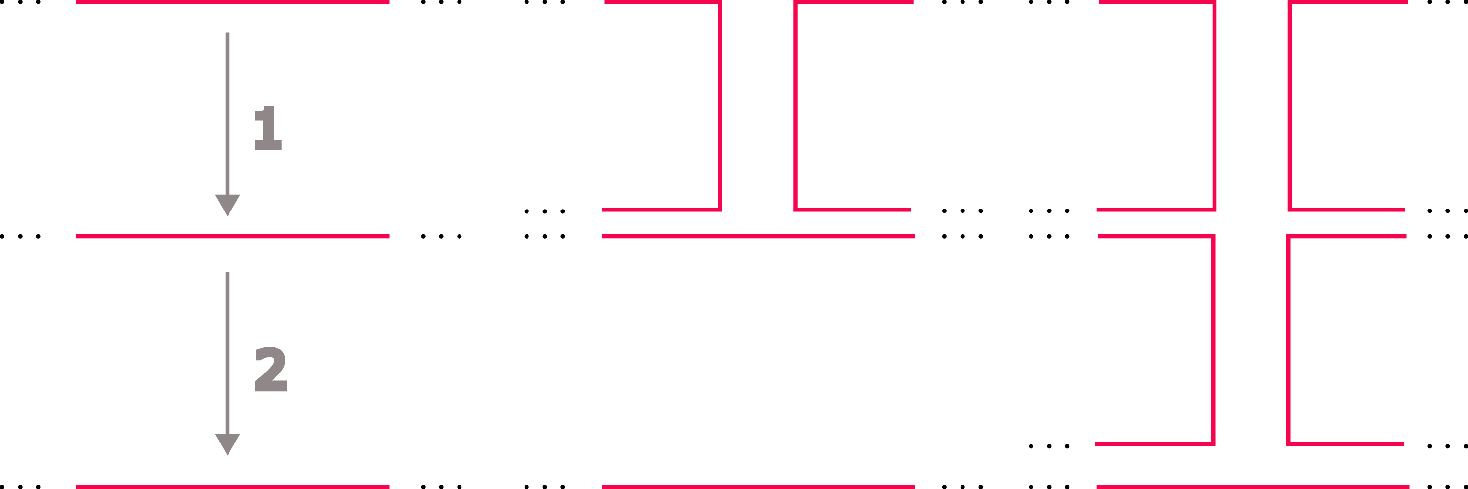
We represent the choice of arcs used for handle slides by using the notation in Figure 9.
Arcs used for handle slides are indicated by arrows as in this figure. The left-hand figure means that firstly we perform the handle slide labelled 1 (the central figure), and then we perform the handle slide labelled 2 (the right-hand figure).

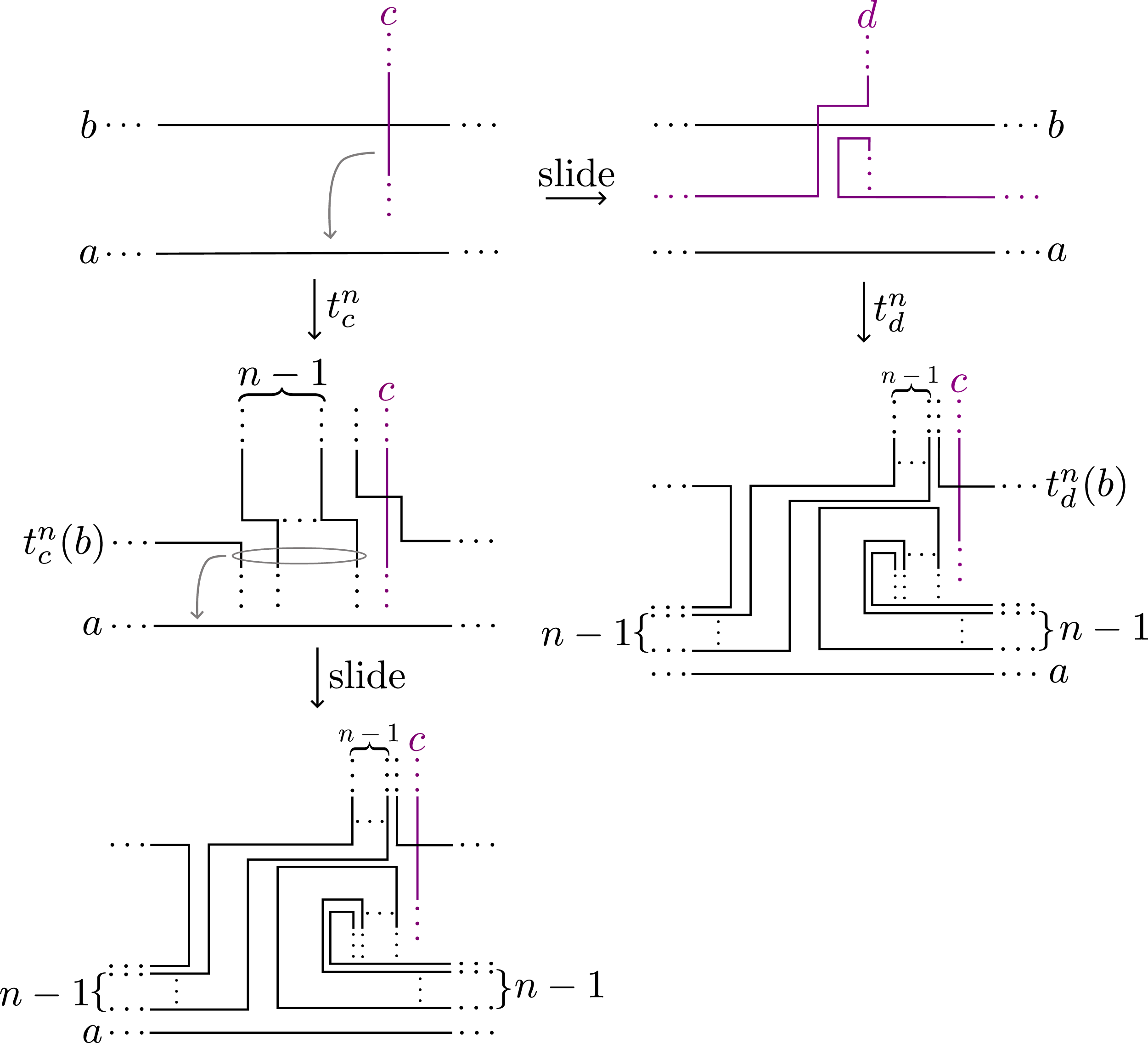
A schematic diagram of Lemma 3·4 in the case where
 $\ell=m=1$
and n is positive.

This figure describes a simple example of Lemma 3·4 for
 $\alpha$
curves of a trisection diagram. In the upper column, we perform firstly the Dehn twist, and then handle sliding as indicated in the figure. This is a usual deformation for trisection diagrams. In the lower column, we firstly handle slide c over the
 $\alpha$
curve in the same way as the upper column, and then perform the Dehn twist. The resulting two
 $\alpha$
curves are the same.

Lemma 3·4. Let a, b and c be simple closed curves in a surface. Suppose that a does not intersect with both of b and c, and that b intersects with c m times. Let d be a simple closed curve obtained by handle sliding c over a
 $\ell$
times along arcs
 $a_1, \ldots, a_\ell$
. Then, for any integer n, the simple closed curve
 $t_d^n(b)$
is isotopic to the simple closed curve obtained by handle sliding
 $t_c^n(b)$
over a
 $\ell \cdot m \cdot \lvert n \rvert$
times along the arcs
 $a_1, \ldots, a_\ell$
.
Proof. A schematic diagram depicted in Figure 10 completes the proof in the case where
 $\ell=m=1$
and n is positive. The other cases can be shown in a similar way.
Remark 3·5. Due to this lemma, we can deform trisection diagrams by handle sliding the twisting curve c over curves of the trisection diagrams while preserving the diffeomorphism types of trisections and 4-manifolds corresponding to the trisection diagrams (see Figure 11 for example). We use this lemma repeatedly in this paper to simplify deformations of trisection diagrams.
Lemma 3·6. The trisection diagram of
 $\Sigma_{S(T(p+1,p))}(S^4)$
shown in Figure 14 can be obtained by destabilising the trisection diagram of
 $\Sigma_{S(T(p+1,p))}(S^4)$
shown in Figure 8 twice.
Proof. In Figure 8, firstly perform
 $t_{\beta_5}^{-1}$
for the entire diagram. Then, handle slide
 $\beta_5$
and the resulting
 $\alpha_5$
over
 $\beta_4$
and
 $\alpha_4$
, respectively, as indicated in Figure 12 (a) to resolve the intersections of the resulting
 $\gamma_5$
and both
 $\beta_5$
and the resulting
 $\alpha_5$
. Then, since
 $\alpha_4$
and
 $\beta_4$
can be parallel by handle slides due to Theorem 2·7, we can destabilise the trisection diagram shown in Figure 8 for
 $\alpha_4$
(precisely
 $t_{\delta_1^{\beta}}^{p-2}t_{\delta_2^{\beta}}^{-(p-2)}(\alpha_4)$
),
 $\beta_4$
(precisely
 $t_{\delta_1^{\beta}}^{p-2}t_{\delta_2^{\beta}}^{-(p-2)}(\beta_4)$
) and the resulting
 $\gamma_5$
. By the destabilisation, we have the trisection diagram
 $\mathcal{D}_1$
obtained by gluing Figure 7 and Figure 12 (b). See also [
Reference Gay and Meier6
, figure 15]. Note that this destabilisation is based on Naylor’s method (Lemma 8 in [
Reference Naylor18
]).
In the trisection diagram
 $\mathcal{D}_1$
, slide
 $\beta_6$
and
 $\gamma_6$
over
 $\beta_5$
and
 $\gamma_4$
, respectively, as indicated in Figure 12 (b). Then, since
 $\gamma_4$
and the resulting
 $\beta_6$
can be parallel by handle slides due to Theorem 2·7 and
 $\delta_i^{\beta}$
can be parallel to
 $\delta_i^{\gamma}$
by sliding
 $\delta_i^{\beta}$
over
 $\beta_2$
in Figure 7 or 8 as indicated in Figure 8 for
 $i=1,2$
, we can destabilise
 $\mathcal{D}_1$
for
 $\alpha_6$
, the resulting
 $\beta_6$
(precisely
 $t_{\delta_1^{\beta}}^{p-2}t_{\delta_2^{\beta}}^{-(p-2)}(\beta_6)$
) and
 $\gamma_4$
(precisely
 $t_{\delta_1^{\gamma}}^{p-2}t_{\delta_2^{\gamma}}^{-(p-2)}(\gamma_4)$
) due to Lemma 3·4. By the destabilisation, we have the trisection diagram
 $\mathcal{D}_2$
obtained by gluing Figure 7 and Figure 13 (c). Note that this destabilisation is also based on Naylor’s method [
Reference Naylor18
, lemma 8].


(Left) A part of the trisection diagram
 $\mathcal{D}_2$
obtained by destabilising the trisection diagram
 $\mathcal{D}_1$
once. (Right) A part of the trisection diagram obtained by performing
 $t_c^{-1}$
for
 $\mathcal{D}_2$
.

A trisection diagram obtained by Gluck twisting on the spun trefoil and the curves
 $\delta_1^{\beta}$
,
 $\delta_2^{\beta}$
,
 $\delta_1^{\gamma}$
and
 $\delta_2^{\gamma}$
. The trisection diagram of
 $\Sigma_{S(T(p+1,p))}(S^4)$
is
 $(\Sigma, \alpha', \beta', \gamma')$
, where
 $\alpha' = (t_{\delta_1^{\beta}}^{p-2}t_{\delta_2^{\beta}}^{-(p-2)}(\alpha_1), \alpha_2, \alpha_3, t_{\delta_1^{\beta}}^{p-2}t_{\delta_2^{\beta}}^{-(p-2)}(\alpha_4))$
,
 $\beta' = (t_{\delta_1^{\beta}}^{p-2}t_{\delta_2^{\beta}}^{-(p-2)}(\beta_1), \beta_2, \beta_3, t_{\delta_1^{\beta}}^{p-2}t_{\delta_2^{\beta}}^{-(p-2)}(\beta_4))$
and
 $\gamma' = (t_{\delta_1^{\gamma}}^{p-2}t_{\delta_2^{\gamma}}^{-(p-2)}(\gamma_1), \gamma_2, \gamma_3, t_{\delta_1^{\gamma}}^{p-2}t_{\delta_2^{\gamma}}^{-(p-2)}(\gamma_4))$
.

The trisection diagram
 $\mathcal{D}_p$
of
 $\Sigma_{S(T(p+1,p))}(S^4)$
, where
 $\alpha = (t_{\delta_1^{\beta}}^{p-2}t_{\delta_2^{\beta}}^{-(p-2)}(\alpha_1),$
 $\alpha_2, \alpha_3, t_{\delta_1^{\beta}}^{p-2}t_{\delta_2^{\beta}}^{-(p-2)}(\alpha_4))$
,
 $\beta = (t_{\delta_1^{\beta}}^{p-2}t_{\delta_2^{\beta}}^{-(p-2)}(\beta_1), \beta_2, \beta_3, t_{\delta_1^{\beta}}^{p-2}t_{\delta_2^{\beta}}^{-(p-2)}(\beta_4))$
and
 $\gamma = (t_{\delta_1^{\gamma}}^{p-2}t_{\delta_2^{\gamma}}^{-(p-2)}$
 $(\gamma_1),\gamma_2, \gamma_3, t_{\delta_1^{\gamma}}^{p-2}t_{\delta_2^{\gamma}}^{-(p-2)}(\gamma_4))$
.

In the trisection diagram
 $\mathcal{D}_2$
, by performing
 $t_c^{-1}$
for Figure 13 (a), we have the trisection diagram obtained by gluing Figure 7 and Figure 13 (b), which is just the trisection diagram shown in Figure 14.
None of the operations above change the diffeomorphism type of the 4-manifold. Thus, the trisection diagram shown in Figure 14 describes the Gluck twisted 4-manifold
 $\Sigma_{S(T(p+1,p))}(S^4)$
. This completes the proof.
In this paper, we will show in Section 4 that the trisection diagram of
 $\Sigma_{S(T(p+1,p))}(S^4)$
in Lemma 3·3 is standard for all
 $p \ge 2$
. Namely, we will prove that the trisection diagram can be related to the genus-0 trisection diagram by surface diffeomorphisms, handle slides and destabilisations. Thus, by Lemma 3·6, it suffices to show that the trisection diagram of
 $\Sigma_{S(T(p+1,p))}(S^4)$
depicted in Figure 14 is standard for all
 $p \ge 2$
.
In Figure 14, we perform the following handle slides in order: slide
 $\alpha_4$
over
 $\alpha_3$
,
 $\alpha_1$
over
 $\alpha_2$
and
 $\alpha_3$
,
 $\alpha_4$
over
 $\alpha_1$
twice,
 $\beta_4$
over
 $\beta_1$
,
 $\beta_1$
over
 $\beta_4$
, and
 $\gamma_4$
over
 $\gamma_1$
twice. These handle slides are indicated in Figure 14. Then, Figure 15 is obtained. Let
 $\mathcal{D}_p$
denote this trisection diagram of
 $\Sigma_{S(T(p+1,p))}(S^4)$
, which is obtained by overlaying all of Figure 15.
4. Main theorem
In this section, we show the following main theorem mentioned in Section 1.
Theorem 4·1. The trisection diagram
 $\mathcal{D}_p$
(
 $p \ge 2$
) is standard.
Proof of Theorem
4·1. The proof is mainly divided into two steps. The first step is that we show the trisection diagram
 $\mathcal{D}_p$
can be destabilised once and destabilise
 $\mathcal{D}_p$
explicitly. The second step is that we reduce the destabilised trisection diagram to the stabilisation of the genus-0 trisection diagram by an inductive argument. As the inductive argument, we use a key lemma which we call the seesaw lemma. Note that we do not change names of simple closed curves before and after Dehn twists and handle slides unless otherwise stated.
Step 1. Destabilise
 $\mathcal{D}_p$
once.
First, we perform Dehn twists
 $t_\epsilon^{p-2}t_\delta^{-1}$
for
 $\mathcal{D}_p$
, where
 $\epsilon$
and
 $\delta$
are curves in Figure 16. At the beginning, we consider
 $\beta$
curves obtained by performing
 $t_\epsilon^{p-2}t_\delta^{-1}$
for the
 $\beta$
curves of
 $\mathcal{D}_p$
. Recall that for a collection of mutually disjoint simple closed curves
 $C=\{c_1, \ldots, c_n\}$
on a surface
 $\Sigma$
,
 $\Sigma_{C}$
denotes the surface obtained by surgering
 $\Sigma$
along C (see theorem 2·7). We say that two simple closed curves a and b on
 $\Sigma$
are equal (
 $a=b$
) up to handle slide over C (or
 $c_1, \ldots, c_{n-1}$
and
 $c_n$
) if they are isotopic on
 $\Sigma_{C}$
.
Lemma 4·2. Let
 $(\Sigma;\;\beta_1^p,\beta_2,\beta_3,\beta_4^p)$
be the
 $\beta$
-curves of
 $\mathcal{D}_p$
, where
 $\beta_1^p=t_{\delta_1^{\beta}}^{p-2}t_{\delta_2^{\beta}}^{-(p-2)}(\beta_1)$
and
 $\beta_4^p=t_{\delta_1^{\beta}}^{p-2}t_{\delta_2^{\beta}}^{-(p-2)}(\beta_4)$
(see Figure 15). Then, the following holds:
-
(i)
$t_\epsilon^{p-2}t_\delta^{-1}(\beta_2)=\beta_2$
and
$t_\epsilon^{p-2}t_\delta^{-1}(\beta_3)=\beta_3$
; -
(ii)
$t_\epsilon^{p-2}t_\delta^{-1}(\beta_4^p)=m$
up to handle slide over
$\beta_2$
; -
(iii)
$t_\epsilon^{p-2}t_\delta^{-1}(\beta_1^p)=t_{\delta_1^{\beta}}^{p-2}(m')$
up to handle slide over
$\beta_2$
and
$\beta_3$
;


where
 $\delta$
,
 $\epsilon$
, m and m’ are the curves depicted in Figure 16.
The
 $\beta$
curves of
 $\mathcal{D}_p$
(Figure 15) and curves
 $\delta$
,
 $\epsilon$
, m and m
′.

Proof. We can immediately check from Figure 16 that
 $t_\epsilon^{p-2}t_\delta^{-1}(\beta_2)=\beta_2$
and
 $t_\epsilon^{p-2}t_\delta^{-1}(\beta_3)=\beta_3$
since
 $\delta$
and
 $\epsilon$
do not intersect with
 $\beta_2$
and
 $\beta_3$
.
First of all, we show the statement for
 $\beta_4^p$
. Since
 $m=t_{\delta}^{-1}(\beta_4)$
and curves
 $\epsilon$
,
 $\delta$
,
 $\delta_1^{\beta}$
and
 $\delta_2^{\beta}$
are all disjoint from
 $\beta_2$
(see Figure 16), it suffices to show that
 $t_{\epsilon}^{p-2} t_{\delta}^{-1} t_{\delta_1^{\beta}}^{p-2}t_{\delta_2^{\beta}}^{-(p-2)}(\beta_4) = t_{\delta}^{-1}(\beta_4)$
up to handle slide over
 $\beta_2$
. Since the geometric intersection number of
 $\delta_1^{\beta}$
and the other curves is 0,
 $t_{\epsilon}^{p-2} t_{\delta}^{-1} t_{\delta_1^{\beta}}^{p-2}t_{\delta_2^{\beta}}^{-(p-2)}(\beta_4) = t_{\delta_1^{\beta}}^{p-2} t_{\epsilon}^{p-2} t_{\delta}^{-1} t_{\delta_2^{\beta}}^{-(p-2)}(\beta_4)$
. Moreover, we can check from Figure 16 that
 $t_{\delta}(\epsilon)=\delta_2^{\beta}$
up to handle slide over
 $\beta_2$
. It is well known that
 $t_{f(c)}=f t_c f^{-1}$
for a simple closed curve c on a surface S and a self-diffeomorphism
 $f : S \to S$
, and that if the geometric intersection number i(a,b) of two simple closed curves a and b is 0, then
 $t_a t_b = t_b t_a$
(for example, see [
Reference Farb and Margalit3
, fact 3·7 and 3·9], respectively). Thus, the following equalities hold up to handle slide over
 $\beta_2$
(Lemma 3·4):
 \begin{eqnarray*}t_{\delta_1^{\beta}}^{p-2} t_{\epsilon}^{p-2} t_{\delta}^{-1} t_{\delta_2^{\beta}}^{-(p-2)}(\beta_4) &=& t_{\delta_1^{\beta}}^{p-2} t_{\delta}^{-1} t_{\delta} t_{\epsilon}^{p-2} t_{\delta}^{-1} t_{\delta_2^{\beta}}^{-(p-2)}(\beta_4)\\&=& t_{\delta_1^{\beta}}^{p-2} t_{\delta}^{-1} t_{t_{\delta}(\epsilon)}^{p-2} t_{\delta_2^{\beta}}^{-(p-2)}(\beta_4)\\&=& t_{\delta_1^{\beta}}^{p-2} t_{\delta}^{-1} t_{\delta_2^{\beta}}^{p-2} t_{\delta_2^{\beta}}^{-(p-2)}(\beta_4)\\&=& t_{\delta}^{-1} t_{\delta_1^{\beta}}^{p-2}(\beta_4).\end{eqnarray*}
Thus, it suffices to show
 $t_{\delta}^{-1} t_{\delta_1^{\beta}}^{p-2}(\beta_4) = t_{\delta}^{-1}(\beta_4)$
. This holds obviously since
 $i(\delta_1^{\beta}, \beta_4) = 0$
(see Figure 16). Next, we show the statement for
 $\beta_1^p$
. We have the following equalities up to handle slide over
 $\beta_2$
(Lemma 3·4):
 \begin{eqnarray*}t_{\delta_1^{\beta}}^{-(p-2)}t_\epsilon^{p-2}t_\delta^{-1}(\beta_1^p) &=& t_{\delta_1^{\beta}}^{-(p-2)}t_\epsilon^{p-2}t_\delta^{-1}t_{\delta_1^{\beta}}^{p-2}t_{\delta_2^{\beta}}^{-(p-2)}(\beta_1)\\&=& t_\delta^{-1}t_{\delta}t_\epsilon^{p-2}t_\delta^{-1}t_{\delta_2^{\beta}}^{-(p-2)}(\beta_1)\\&=& t_\delta^{-1}t_{t_{\delta}(\epsilon)}^{p-2}t_{\delta_2^{\beta}}^{-(p-2)}(\beta_1)\\&=& t_\delta^{-1}t_{\delta_2^{\beta}}^{p-2}t_{\delta_2^{\beta}}^{-(p-2)}(\beta_1)\\&=& t_{\delta}^{-1}(\beta_1).\end{eqnarray*}
We see from Figure 16 that
 $t_{\delta}^{-1}(\beta_1)$
can be parallel to m
′ after handle sliding over both
 $\beta_2$
and
 $\beta_3$
as indicated in Figure 16. This completes the proof.
Next, we consider
 $\alpha$
curves obtained by performing
 $t_\epsilon^{p-2}t_\delta^{-1}$
for the
 $\alpha$
curves of
 $\mathcal{D}_p$
(Figure 15 or 19). Recall that the
 $\alpha$
curves of
 $\mathcal{D}_p$
are
 $(t_{\delta_1^{\beta}}^{p-2}t_{\delta_2^{\beta}}^{-(p-2)}(\alpha_1), \alpha_2, \alpha_3, t_{\delta_1^{\beta}}^{p-2}t_{\delta_2^{\beta}}^{-(p-2)}(\alpha_4))$
. Before deforming the
 $\alpha$
curves, we define the following operation including the Dehn twists, which we call
 $\ast_\alpha$
: first, perform
 $t_{\delta}^{-1}$
. Then, slide the resulting
 $\alpha_1$
(i.e.
 $t_{\delta}^{-1}t_{\delta_1^{\beta}}^{p-2}t_{\delta_2^{\beta}}^{-(p-2)}(\alpha_1)$
) over the resulting
 $\alpha_3$
(i.e.
 $t_{\delta}^{-1}(\alpha_3)$
, which is the
 $\alpha_3$
depicted in the left-hand side of Figure 17) only once as indicated in the left-hand side of Figure 17 to resolve the intersection of the resulting
 $\alpha_1$
and
 $\epsilon$
. After that, perform
 $t_{\epsilon}^{p-2}$
. Finally, slide the resulting
 $\alpha_1$
(the
 $\alpha_1$
depicted in the right-hand side of Figure 17) and the resulting
 $\alpha_3$
(i.e.
 $t_{\epsilon}^{p-2}t_{\delta}^{-1}(\alpha_3)$
, which is the
 $\alpha_3$
depicted in the right-hand side of Figure 17) over the resulting
 $\alpha_4$
(i.e.
 $t_{\epsilon}^{p-2}t_{\delta}^{-1}t_{\delta_1^{\beta}}^{p-2}t_{\delta_2^{\beta}}^{-(p-2)}(\alpha_4)$
, which is the
 $\alpha_4$
depicted in the right-hand side of Figure 17)
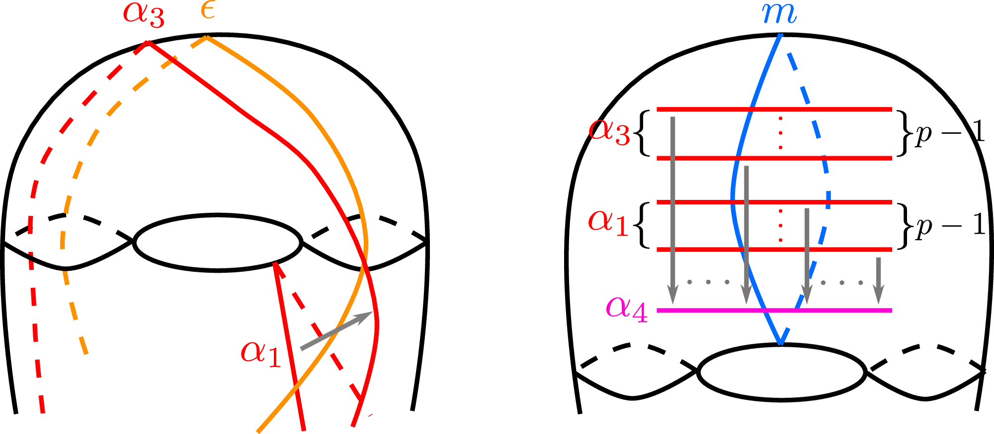
 $p-1$
times each as indicated in the right-hand side of Figure 17 to resolve the intersections of m and both the resulting
 $\alpha_1$
and the resulting
 $\alpha_3$
.
These figures describe how to perform the handle slides in the operation
 $\ast_\alpha$
. In the left-hand figure,
 $\alpha_1$
and
 $\alpha_3$
precisely represent
 $t_{\delta}^{-1}t_{\delta_1^{\beta}}^{p-2}t_{\delta_2^{\beta}}^{-(p-2)}(\alpha_1)$
and
 $t_{\delta}^{-1}(\alpha_3)$
, respectively, for the
 $\alpha$
curves of
 $\mathcal{D}_p$
(i.e.
 $\alpha_1$
and
 $\alpha_3$
in Figure 15 or 19). In the right-hand figure,
 $\alpha_3$
and
 $\alpha_4$
precisely represent
 $t_{\epsilon}^{p-2}t_{\delta}^{-1}(\alpha_3)$
and
 $t_{\epsilon}^{p-2}t_{\delta}^{-1}t_{\delta_1^{\beta}}^{p-2}t_{\delta_2^{\beta}}^{-(p-2)}(\alpha_4)$
, respectively, for the
 $\alpha$
curves of
 $\mathcal{D}_p$
(i.e.
 $\alpha_3$
and
 $\alpha_4$
in Figure 15 or 19). The
 $\alpha_1$
in the right-hand figure precisely represents the curve obtained by performing
 $t_{\epsilon}^{p-2}$
for the curve c obtained by sliding the
 $\alpha_1$
in the left-hand figure over the
 $\alpha_3$
in the left-hand figure as indicated in the left-hand figure. In fact,
 $t_{\epsilon}^{p-2}(c)=c$
since
 $\epsilon$
does not intersect with c due to the slide in the left-hand figure.


Lemma 4·3. The
 $\alpha$
curves
 $(t_{\delta_1^{\beta}}^{p-2}t_{\hat{\delta}}^{-(p-2)}(\alpha_1), \alpha_2, t_{\delta_1^{\beta}}^{p-2}t_{\tilde{\delta}}^{p-2}(\alpha_3), t_{\delta_1^{\beta}}^{p-2}(\alpha_4))$
can be obtained by performing the operation
 $\ast_\alpha$
for the
 $\alpha$
curves of
 $\mathcal{D}_p$
in Figure 15, where
 $\alpha_1$
,
 $\alpha_3$
,
 $\hat{\delta}$
and
 $\tilde{\delta}$
are the curves depicted in Figure 18.
Proof. It is obvious that
 $t_{\delta_1^{\beta}}^{p-2}(\alpha_4)$
is obtained by
 $\ast_\alpha$
since both
 $\delta$
and
 $\epsilon$
do not intersect with
 $\alpha_4$
and
 $\delta_1^{\beta}$
(see Figure 19).
We show firstly the statement for
 $\alpha_1$
. Since
 $\delta_1^{\beta}$
does not intersect with
 $\delta_2^{\beta}$
,
 $\delta$
and
 $\epsilon$
(see Figure 19), the operations in
 $\ast_\alpha$
which deform
 $\alpha_1$
in Figure 15 can be considered as follows: First, perform
 $t_{\delta_2^{\beta}}^{-(p-2)}$
and
 $t_{\delta}^{-1}$
in order. Then, slide the resulting
 $\alpha_1$
over
 $t_{\delta}^{-1}(\alpha_3)$
as indicated in the left-hand side of Figure 17. After that, slide the resulting
 $\alpha_1$
over
 $\alpha_4$
 $p-1$
times as indicated in the right-hand side of Figure 17. Finally, perform
 $t_{\delta_1^{\beta}}^{p-2}$
.
The
 $\alpha$
curves of
 $\mathcal{D}_p$
(Figure 15) and curves
 $\delta$
and
 $\epsilon$
.

Since
 $t_{\delta}^{-1}t_{\delta_2^{\beta}}^{-(p-2)}=t_{t_{\delta}^{-1}(\delta_2^{\beta})}^{-(p-2)}t_{\delta}^{-1}$
, we can take the following operations for
 $\alpha_1$
instead of the above operations: first, perform
 $t_{\delta}^{-1}$
and
 $t_{t_{\delta}^{-1}(\delta_2^{\beta})}^{-(p-2)}$
in order. Then, slide the resulting
 $\alpha_1$
over the resulting
 $\alpha_3$
(i.e.
 $t_{\delta}^{-1}(\alpha_3)$
) as indicated in the left-hand side of Figure 17. After that, slide the resulting
 $\alpha_1$
over
 $\alpha_4$
 $p-1$
times as indicated in the right-hand side of Figure 17. Finally, perform
 $t_{\delta_1^{\beta}}^{p-2}$
.
The first operation
 $t_{\delta}^{-1}$
does not deform
 $\alpha_1$
in Figure 15 since
 $\delta$
does not intersect with
 $\alpha_1$
(see Figure 19). Thus, we can take the following operations: first, perform
 $t_{t_{\delta}^{-1}(\delta_2^{\beta})}^{-(p-2)}$
. Then, slide the resulting
 $\alpha_1$
over
 $t_{\delta}^{-1}(\alpha_3)$
as indicated in the left-hand side of Figure 17. After that, slide the resulting
 $\alpha_1$
over
 $\alpha_4$
 $p-1$
times as indicated in the right-hand side of Figure 17. Finally, perform
 $t_{\delta_1^{\beta}}^{p-2}$
.
In these operations, since
 $t_{\delta}^{-1}(\delta_2^{\beta})$
does not intersect with
 $t_{\delta}^{-1}(\alpha_3)$
and
 $\alpha_4$
in Figure 15 or 19, we can change the order in the operations as follows: first, slide the
 $\alpha_1$
over
 $t_{\delta}^{-1}(\alpha_3)$
and
 $\alpha_4$
once each as indicated in the left-hand side of Figure 17 and right-hand side of Figure 17, respectively. Then, perform
 $t_{t_{\delta}^{-1}(\delta_2^{\beta})}^{-(p-2)}$
. After that, slide the resulting
 $\alpha_1$
over
 $\alpha_4$
 $p-2$
times as indicated in the right-hand side of Figure 17. Finally, perform
 $t_{\delta_1^{\beta}}^{p-2}$
.
The first operation, namely, handle sliding
 $\alpha_1$
over
 $t_{\delta}^{-1}(\alpha_3)$
and
 $\alpha_4$
, provides us with
 $\alpha_1$
in Figure 18 (a) up to handle slide over
 $\alpha_2$
. Thus, the remaining operations for
 $\alpha_1$
in Figure 18 (a) are as follows: first, perform
 $t_{t_{\delta}^{-1}(\delta_2^{\beta})}^{-(p-2)}$
. After that, slide the resulting
 $\alpha_1$
over
 $\alpha_4$
 $p-2$
times as indicated in the right-hand side of Figure 17. Finally, perform
 $t_{\delta_1^{\beta}}^{p-2}$
.
Since the simple closed curve
 $t_{\delta}^{-1}(\delta_2^{\beta})$
does not intersect with
 $\alpha_4$
and
 $t_{\delta}^{-1}(\delta_2^{\beta})$
intersects with
 $\alpha_1$
in Figure 18 (a) once, the first two operations can be regarded as an operation that performs
 $t_c^{-(p-2)}$
due to Lemma 3·4, where c is the simple closed curve obtained by sliding
 $t_{\delta}^{-1}(\delta_2^{\beta})$
over
 $\alpha_4$
as indicated in the right-hand side of Figure 17. Actually, c is
 $\hat{\delta}$
. Recall that
 $\hat{\delta}$
is the curve depicted in Figure 18 (a). This completes the proof for
 $\alpha_1$
.
Next, we show the statement for
 $\alpha_3$
. In the operation
 $\ast_\alpha$
, the operations which deform
 $\alpha_3$
in Figure 15 are as follows: first, perform
 $t_{\delta}^{-1}$
and
 $t_{\epsilon}^{p-2}$
in order. After that, slide the resulting
 $\alpha_3$
over
 $\alpha_4$
 $p-1$
times as indicated in the right-hand side of Figure 17. Finally, perform
 $t_{\delta_1^{\beta}}^{p-2}$
.
Since
 $\delta$
and
 $\epsilon$
does not intersect with
 $\alpha_4$
, we can regard these operations as the following operations due to Lemma 3·4: perform
 $t_{c_1}^{-1}$
,
 $t_{c_2}^{p-2}$
and
 $t_{\delta_1^{\beta}}^{p-2}$
in order, where
 $c_1$
is the simple closed curve obtained by handle sliding
 $\delta$
over
 $\alpha_4$
once as indicated in the right-hand side of Figure 17 (in Figure 19 explicitly) and
 $c_2$
is the simple closed curve obtained by handle sliding
 $\epsilon$
over
 $\alpha_4$
once as indicated in the right-hand side of Figure 17 (in Figure 19 explicitly). It is obvious that
 $t_{c_1}^{-1}(\alpha_3)$
for
 $\alpha_3$
in Figure 15 is
 $\alpha_3$
in Figure 18 (b) and
 $c_2$
is
 $\tilde{\delta}$
. Recall that
 $\tilde{\delta}$
is the curve depicted in Figure 18 (b). This completes the proof for
 $\alpha_3$
.
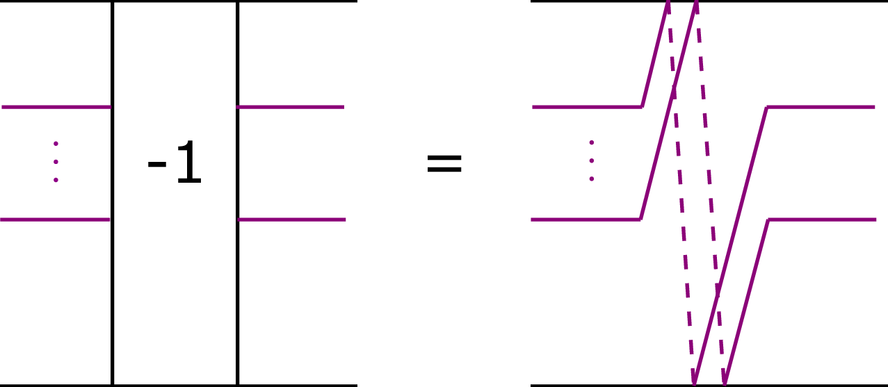
A simple notation for trisection diagrams based on the twist-box notations in Kirby diagrams. This notation simplifies the left-handed Dehn twist.

Lastly, we consider
 $\gamma$
curves obtained by performing
 $t_\epsilon^{p-2}t_\delta^{-1}$
for the
 $\gamma$
curves of
 $\mathcal{D}_p$
(Figure 15 or 22). Recall that the
 $\gamma$
curves of
 $\mathcal{D}_p$
are
 $(t_{\delta_1^{\gamma}}^{p-2}t_{\delta_2^{\gamma}}^{-(p-2)}(\gamma_1), \gamma_2, \gamma_3, t_{\delta_1^{\gamma}}^{p-2}t_{\delta_2^{\gamma}}^{-(p-2)}(\gamma_4))$
for
 $\delta_1^{\gamma}$
and
 $\delta_2^{\gamma}$
in Figure 15 or 22. Before deforming the
 $\gamma$
curves, we define the following operation including the Dehn twists, which we call
 $\ast_\gamma$
: first, slide
 $\delta_1^{\gamma}$
in Figure 15 or 22 over
 $\gamma_3$
of
 $\mathcal{D}_p$
(Figure 22) as indicated in Figure 22. By this handle slide,
 $\delta_1^{\gamma}$
in Figure 21 is obtained. Thus, the
 $\gamma$
curves of
 $\mathcal{D}_p$
can be regarded as
 $(t_{\delta_1^{\gamma}}^{p-2}t_{\delta_2^{\gamma}}^{-(p-2)}(\gamma_1), \gamma_2, \gamma_3, t_{\delta_1^{\gamma}}^{p-2}t_{\delta_2^{\gamma}}^{-(p-2)}(\gamma_4))$
for
 $\delta_1^{\gamma}$
in Figure 21 and
 $\delta_2^{\gamma}$
in Figure 15 or 22 due to Lemma 3·4. Then, perform
 $t_{\delta}^{-1}$
and
 $t_{\epsilon}^{p-2}$
in order for the resulting
 $\gamma$
curves. After that, slide the resulting
 $\gamma_3$
(i.e.
 $t_{\epsilon}^{p-2}t_{\delta}^{-1}(\gamma_3)$
in Figure 22) over the resulting
 $t_{{\delta_1^\gamma}}^{p-2} t_{{\delta_2^\gamma}}^{-(p-2)}(\gamma_4)$
(i.e.
 $t_\epsilon^{p-2}t_\delta^{-1}$
 $t_{{\delta_1^\gamma}}^{p-2} t_{{\delta_2^\gamma}}^{-(p-2)}(\gamma_4)$
in Figure 22, where only
 $\delta_1^\gamma$
is the curve in Figure 21) only once to resolve the intersection with m in Figure 16. The way of performing the handle slide is similar to the last slide in the operation
 $\ast_\alpha$
(see the right-hand side of Figure 17). Note that the resulting
 $t_{{\delta_1^\gamma}}^{p-2} t_{{\delta_2^\gamma}}^{-(p-2)}(\gamma_4)$
intersects with m only once since the equations
 $t_\epsilon^{p-2}t_\delta^{-1} t_{{\delta_1^\gamma}}^{p-2} t_{{\delta_2^\gamma}}^{-(p-2)}(\gamma_4) = t_{{\delta_1^\gamma}}^{p-2} t_{\delta}^{-1}(\gamma_4) = t_{{\delta_1^\gamma}}^{p-2}(\gamma_4)$
hold (see the proof of Lemma 4·4),
 ${\delta_1^\gamma}$
does not intersect with m and
 $\gamma_4$
in Figure 15 or 22 intersects with m once.
Lemma 4·4. The
 $\gamma$
curves
 $(t_{{\delta_1^\gamma}}^{p-2}(\gamma_1), \gamma_2, t_{{\delta_1^\gamma}}^{p-2}(\gamma_3), t_{{\delta_1^\gamma}}^{p-2}(\gamma_4))$
can be obtained by performing the operation
 $\ast_\gamma$
for the
 $\gamma$
curves of
 $\mathcal{D}_p$
in Figure 15, where
 $\gamma_1$
,
 $\gamma_3$
, and
 $\delta_1^\gamma$
are the curves depicted in Figure 21.
Proof. We can check from Figure 22 that
 $t_{\delta}(\epsilon)=\delta_2^{\gamma}$
and
 $\delta_1^{\gamma}$
in Figure 21 does not intersect with
 $\delta_2^{\gamma}$
,
 $\delta$
and
 $\epsilon$
. Thus, for
 $\delta_1^{\gamma}$
in Figure 21 and
 $\delta_2^{\gamma}$
,
 $\delta$
and
 $\epsilon$
in Figure 22, we have
A part of the
 $\gamma$
curves obtained by the operation
 $\ast_\gamma$
for the
 $\gamma$
curves of
 $\mathcal{D}_p$
(Figure 15).

The
 $\gamma$
curves of
 $\mathcal{D}_p$
(Figure 15) and curves
 $\delta$
and
 $\epsilon$
.

 \begin{eqnarray*}t_{\epsilon}^{p-2} t_{\delta}^{-1} t_{{\delta_1^\gamma}}^{p-2} t_{{\delta_2^\gamma}}^{-(p-2)}&=& t_{{\delta_1^\gamma}}^{p-2} t_{\epsilon}^{p-2} t_{\delta}^{-1} t_{{\delta_2^\gamma}}^{-(p-2)}\\&=& t_{{\delta_1^\gamma}}^{p-2} t_{\delta}^{-1} t_{t_{\delta}(\epsilon)}^{p-2} t_{{\delta_2^\gamma}}^{-(p-2)}\\&=& t_{{\delta_1^\gamma}}^{p-2} t_{\delta}^{-1} t_{{\delta_2^\gamma}}^{p-2} t_{{\delta_2^\gamma}}^{-(p-2)}\\&=& t_{{\delta_1^\gamma}}^{p-2} t_{\delta}^{-1}.\end{eqnarray*}
Therefore, the statement for
 $\gamma_1$
,
 $\gamma_2$
and
 $\gamma_4$
obviously holds since
 $\delta$
does not intersect with
 $\gamma_1$
,
 $\gamma_2$
and
 $\gamma_4$
in Figure 22.
For
 $\gamma_3$
, we may consider the following operations: first, perform
 $t_{\delta}^{-1}$
and
 $t_{{\delta_1^\gamma}}^{p-2}$
in order. Then, slide the resulting
 $\gamma_3$
(i.e.
 $t_{{\delta_1^\gamma}}^{p-2}t_{\delta}^{-1}(\gamma_3)$
) over
 $t_{{\delta_1^\gamma}}^{p-2}(\gamma_4)$
 $(= t_{{\delta_1^\gamma}}^{p-2}t_{\delta}^{-1}(\gamma_4) )$
as indicated in the right-hand side of Figure 17.
We can take the following operations instead of the above operations: first, perform
 $t_{\delta}^{-1}$
. Then, slide the resulting
 $\gamma_3$
(i.e.
 $t_{\delta}^{-1}(\gamma_3)$
) over
 $\gamma_4$
 $(= t_{\delta}^{-1}(\gamma_3) )$
as indicated in the right-hand side of Figure 17. After that, perform
 $t_{{\delta_1^\gamma}}^{p-2}$
.
We see that the simple closed curve obtained by handle sliding
 $t_{\delta}^{-1}(\gamma_3)$
in Figure 15 (or Figure 22) over
 $\gamma_4$
as indicated in the right-hand side of Figure 17 is
 $\gamma_3$
in Figure 21. This completes the proof.
So, due to Lemmas 4·2, 4·3 and 4·4, we now have the trisection diagram
 $(\Sigma;\; \alpha, \beta, \gamma)$
of the Gluck twisted 4-manifold
 $\Sigma_{S(T(p+1,p))}(S^4)$
, where
 $\alpha = (t_{\delta_1^{\beta}}^{p-2}t_{\hat{\delta}}^{-(p-2)}(\alpha_1), \alpha_2, t_{\delta_1^{\beta}}^{p-2}t_{\tilde{\delta}}^{p-2}(\alpha_3), t_{\delta_1^{\beta}}^{p-2}(\alpha_4))$
,
 $\beta = (t_{\delta_1^{\beta}}^{p-2}(m'), \beta_2, \beta_3, \beta_4=m)$
and
 $\gamma = (t_{{\delta_1^\gamma}}^{p-2}(\gamma_1), \gamma_2, t_{{\delta_1^\gamma}}^{p-2}(\gamma_3), t_{{\delta_1^\gamma}}^{p-2}(\gamma_4))$
(see Figures 18, 16 and 21, respectively). Recall that
 $\hat{\delta}$
and
 $\tilde{\delta}$
are the curves depicted in Figure 18. Then,
 $\beta_4 = m$
intersects both
 $\alpha_4$
and
 $\gamma_4$
only once. By handle sliding
 $\alpha_4$
and
 $\gamma_4$
over
 $\alpha_2$
and
 $\gamma_2$
, respectively, as indicated in Figure 23,
 $\alpha_4$
and
 $\gamma_4$
can be parallel. Moreover,
 $\delta_1^{\beta}$
and
 $\delta_1^{\gamma}$
can be parallel by the same handle slide (Figure 23). Thus,
 $t_{\delta_1^{\beta}}^{p-2}(\alpha_4)$
and
 $t_{{\delta_1^\gamma}}^{p-2}(\gamma_4)$
can be parallel (slide other curves if necessary), and we can destabilise the trisection diagram for
 $t_{\delta_1^{\beta}}^{p-2}(\alpha_4)$
,
 $\beta_4$
and
 $t_{{\delta_1^\gamma}}^{p-2}(\gamma_4)$
due to Lemma 3·4. Note that this destabilisation is based on Naylor’s method (Lemma 8 in [
Reference Naylor18
]). By this destabilisation, we now have the trisection diagram
 $(\Sigma;\; \alpha, \beta, \gamma)$
depicted in Figure 24, where
 $\alpha = (t_{\delta_1^{\beta}}^{p-2}t_{\hat{\delta}}^{-(p-2)}(\alpha_1), \alpha_2, t_{\delta_1^{\beta}}^{p-2}t_{\tilde{\delta}}^{p-2}(\alpha_3))$
,
 $\beta = (t_{\delta_1^{\beta}}^{p-2}(\beta_1), \beta_2, \beta_3)$
and
 $\gamma = (t_{{\delta_1^\gamma}}^{p-2}(\gamma_1), \gamma_2, t_{{\delta_1^\gamma}}^{p-2}(\gamma_3))$
.


The trisection diagram obtained by the destabilisation in the step 1, where
 $\alpha=(t_{\delta_1^{\beta}}^{p-2} t_{\hat{\delta}}^{-(p-2)} (\alpha_1), \alpha_2, t_{\delta_1^{\beta}}^{p-2} t_{\tilde{\delta}}^{p-2} (\alpha_3))$
,
 $\beta=(t_{\delta_1^{\beta}}^{p-2}(\beta_1), \beta_2, \beta_3)$
and
 $\gamma=(t_{\delta_1^{\gamma}}^{p-2} (\gamma_1), \gamma_2, t_{\delta_1^{\gamma}}^{p-2} (\gamma_3))$
.

Step 2. Reduce the destabilised trisection diagram to the stabilisation of the genus-0 trisection diagram.
We make some preparations to adapt the seesaw lemma (Lemma 4·6). In Figure 24, slide
 $\gamma_3$
over
 $\gamma_1$
as indicated in Figure 24 (labeled 1), perform
 $t_{\beta_2}$
for the entire diagram and slide
 $\alpha_1$
over
 $\alpha_2$
as indicated in Figure 24. Then, the trisection diagram
 $(\Sigma;\; \alpha, \beta, \gamma)$
depicted in Figure 25, where
 $\alpha = (t_{\delta_1^{\beta}}^{p-2}t_{\hat{\delta}}^{-(p-2)}(\alpha_1), \alpha_2, t_{\delta_1^{\beta}}^{p-2}t_{\tilde{\delta}}^{p-2}(\alpha_3))$
,
 $\beta = (t_{\delta_1^{\gamma}}^{p-2}(\beta_1), \beta_2, \beta_3)$
and
 $\gamma = (t_{{\delta_1^\gamma}}^{p-2}(\gamma_1), \gamma_2, t_{{\delta_1^\gamma}}^{p-2}(\gamma_3))$
, can be obtained. Note that we here slide
 $\delta_1^\beta$
and
 $\delta_1^\gamma$
over
 $\beta_2$
and the new
 $\gamma_3$
(i.e.
 $\gamma_3$
in Figure 25), respectively, as indicated in Figure 24 (Lemma 3·4). Let
 $g(\gamma)$
denotes
 $(g(\gamma_1), g(\gamma_2), g(\gamma_3))$
for a surface diffeomorphism g and a collection of simple closed curves
 $\gamma=(\gamma_1,\gamma_2,\gamma_3)$
.
Lemma 4·5. The trisection diagram
 $(\Sigma;\; \alpha, \beta, \gamma)$
depicted in Figure 26, where
 $\alpha = (\alpha_1, \alpha_2, \alpha_3)$
,
 $\beta = (\beta_1, \beta_2, \beta_3)$
and
 $\gamma = t_{\tilde{\delta}}^{-(p-2)} t_{\hat{\delta}}^{p-2} t_{\delta_1^{\beta}}^{-(p-2)} t_{{\delta_1^\gamma}}^{p-2}(\gamma_1, \gamma_2, \gamma_3)$
, can be obtained from the trisection diagram depicted in Figure 25.
Proof. By performing
 $t_{\tilde{\delta}}^{-(p-2)} t_{\hat{\delta}}^{p-2} t_{\delta_1^{\beta}}^{-(p-2)}$
for the trisection diagram depicted in Figure 25, we have the trisection diagram
 \[(\Sigma;\; \alpha, t_{\tilde{\delta}}^{-(p-2)} t_{\hat{\delta}}^{p-2} t_{\delta_1^{\beta}}^{-(p-2)}t_{{\delta_1^\gamma}}^{p-2}(\beta), t_{\tilde{\delta}}^{-(p-2)} t_{\hat{\delta}}^{p-2} t_{\delta_1^{\beta}}^{-(p-2)}t_{{\delta_1^\gamma}}^{p-2}(\gamma)),\]
where
 $\alpha = (\alpha_1,\alpha_2,\alpha_3)$
,
 $\beta= (\beta_1,\beta_2,\beta_3)$
and
 $\gamma = (\gamma_1,\gamma_2,\gamma_3)$
in Figure 25 and
 $\tilde{\delta}$
,
 $\hat{\delta}$
,
 $\delta_1^{\beta}$
and
 $\delta_1^{\gamma}$
are the curves in Figure 25. By sliding
 $\alpha_3$
over
 $\alpha_1$
as indicated in Figure 25, we have the
 $\alpha$
curves in Figure 26. By sliding
 $\hat{\delta}$
and
 $\delta_1^{\beta}$
over
 $\beta_2$
as indicated in Figures 25 and 24 (b), respectively,
 $\hat{\delta}$
and
 $\delta_1^{\beta}$
can be parallel to
 $\tilde{\delta}$
and
 ${\delta_1^\gamma}$
, respectively. Thus,
 $t_{\tilde{\delta}}^{-(p-2)} t_{\hat{\delta}}^{p-2} t_{\delta_1^{\beta}}^{-(p-2)}t_{{\delta_1^\gamma}}^{p-2}(\beta_1,\beta_2,\beta_3)$
can be regarded as the
 $\beta$
curves
 $(\beta_1,\beta_2,\beta_3)$
in Figure 26 due to Lemma 3·4. In the
 $\gamma$
curves,
 $\tilde{\delta}$
and
 $\hat{\delta}$
in Figure 26 is obtained by sliding
 $\tilde{\delta}$
and
 $\hat{\delta}$
in Figure 25 over
 $\gamma_2$
as indicated in Figure 25 (Lemma 3·4). This completes the proof.
In Figure 26,
 $\hat{\delta} = t_{m}^{-1}(\delta_1^{\beta})$
and
 $\tilde{\delta} = t_{m}^{-1}(\delta_1^{\gamma})$
. Thus,
 $t_{\tilde{\delta}}^{-(p-2)} t_{\hat{\delta}}^{p-2} t_{\delta_1^{\beta}}^{-(p-2)} t_{{\delta_1^\gamma}}^{p-2} = t_{m}^{-1} t_{f_{p-2}(m)}$
, where
 $f_{p-2}= t_{\delta_1^{\beta}}^{-(p-2)} t_{{\delta_1^\gamma}}^{p-2} = {(t_{\delta_1^{\beta}}^{-1} t_{{\delta_1^\gamma}})}^{p-2}$
. Here, the trisection diagram
 $(\Sigma;\; \alpha, \beta, t_{m}^{-1} t_{f_{p-2}(m)}(\gamma))$
is obtained from Lemma 4·5. Then,
 $(\Sigma;\; \alpha, \beta, t_{f_{p-2}(m)}(\gamma))$
is obtained by performing
 $t_m$
for the trisection diagram
 $(\Sigma;\; \alpha, \beta, t_{m}^{-1} t_{f_{p-2}(m)}(\gamma))$
. For this trisection diagram
 $(\Sigma;\; \alpha, \beta, t_{f_{p-2}(m)}(\gamma))$
, the following key lemma holds, which we call the seesaw lemma.
The trisection diagram obtained from Figure 24 after some handle slides and Dehn twists, where
 $\alpha = (t_{\delta_1^{\beta}}^{p-2}t_{\hat{\delta}}^{-(p-2)}(\alpha_1), \alpha_2, t_{\delta_1^{\beta}}^{p-2}t_{\tilde{\delta}}^{p-2}(\alpha_3))$
,
 $\beta = (t_{\delta_1^{\gamma}}^{p-2}(\beta_1), \beta_2, \beta_3)$
and
 $\gamma = (t_{{\delta_1^\gamma}}^{p-2}(\gamma_1), \gamma_2, t_{{\delta_1^\gamma}}^{p-2}(\gamma_3))$
. In the figure of the
 $\beta$
curves, a part of
 $\hat{\delta}$
in the figure of the
 $\alpha$
curves is depicted. In the figure of the
 $\gamma$
curves, parts of
 $\tilde{\delta}$
and
 $\hat{\delta}$
in the figure of the
 $\alpha$
curves are depicted.

Lemma 4·6 (The seesaw lemma). Let
 $\alpha=(\alpha_1,\alpha_2,\alpha_3)$
,
 $\beta=(\beta_1,\beta_2,\beta_3)$
and
 $\gamma=(\gamma_1,\gamma_2,\gamma_3)$
in Figure 26. Then, the trisection diagrams
 $(\Sigma;\; \alpha, \beta, t_{f_{p-2}(m)}(\gamma))$
and
 $(\Sigma;\; \alpha, t_{m'}(\beta), t_{f_{p-3}(m)}(\gamma))$
are related by surface diffeomorphisms and handle slides.
The trisection diagram obtained in Lemma 4·4, where
 $\alpha=(\alpha_1,\alpha_2,\alpha_3)$
,
 $\beta=(\beta_1,\beta_2,\beta_3)$
,
 $\gamma=t_{f_{p-2}(m)}(\gamma_1,\gamma_2,\gamma_3)$
and
 $f_{p-2}= t_{\delta_1^{\beta}}^{-(p-2)} t_{{\delta_1^\gamma}}^{p-2} = {(t_{\delta_1^{\beta}}^{-1} t_{{\delta_1^\gamma}})}^{p-2}$
.

Proof. We focus on the simple closed curve
 $f_{p-2}(m)$
. By performing
 $t_{f_{p-2}(m)}^{-1}$
for
 $(\Sigma;\; \alpha, \beta, t_{f_{p-2}(m)}(\gamma))$
,
 $(\Sigma;\; t_{f_{p-2}(m)}^{-1}(\alpha), t_{f_{p-2}(m)}^{-1}(\beta), \gamma)$
is obtained. Then, since
 $f_{p-2}(m)$
can be parallel to m by sliding
 $f_{p-2}(m)$
over
 $\beta_2$
 $p-2$
times as indicated in Figure 24 (b),
 $(\Sigma;\; t_{f_{p-2}(m)}^{-1}(\alpha), \beta, \gamma)$
is obtained from
 $(\Sigma;\; t_{f_{p-2}(m)}^{-1}(\alpha), t_{f_{p-2}(m)}^{-1}(\beta), \gamma)$
by the handle slides due to Lemma 3·4. In the
 $\alpha$
curves,
 $f_{p-2}(m')$
is obtained by sliding
 $f_{p-2}(m)$
over
 $\alpha_2$
as indicated in Figure 23 (a). Thus,
 $(\Sigma;\; t_{f_{p-2}(m')}^{-1}(\alpha), \beta, \gamma)$
is obtained from
 $(\Sigma;\; t_{f_{p-2}(m)}^{-1}(\alpha), \beta, \gamma)$
by the handle slide due to Lemma 3·4. By performing
 $t_{f_{p-2}(m')}$
for
 $(\Sigma;\; t_{f_{p-2}(m')}^{-1}(\alpha), \beta, \gamma)$
,
 $(\Sigma;\; \alpha, t_{f_{p-2}(m')}(\beta), t_{f_{p-2}(m')}(\gamma))$
is obtained. In the
 $\beta$
curves, since
 $f_{p-2}(m')$
can be parallel to m
′ by sliding
 $f_{p-2}(m')$
over
 $\beta_2$
 $p-2$
times as indicated in Figure 25,
 $(\Sigma;\; \alpha, t_{m'}(\beta), t_{f_{p-2}(m')}(\gamma))$
is obtained from
 $(\Sigma;\; \alpha, t_{f_{p-2}(m')}(\beta), t_{f_{p-2}(m')}(\gamma))$
by the handle slides due to Lemma 3·4. Moreover, in the
 $\gamma$
curves,
 $f_{p-2}(m')$
can be parallel to
 $f_{p-3}(m)$
by sliding
 $f_{p-2}(m')$
over
 $\gamma_2$
as indicated in
 $\hat{\delta}$
of Figure 25 since
 $f_1(m')$
can be parallel to m by sliding
 $f_1(m')$
over
 $\gamma_2$
as indicated in
 $\hat{\delta}$
of Figure 25. Thus,
 $(\Sigma;\; \alpha, t_{m'}(\beta), t_{f_{p-3}(m)}(\gamma))$
is obtained from
 $(\Sigma;\; \alpha, t_{m'}(\beta), t_{f_{p-2}(m')}(\gamma))$
by the handle slide due to Lemma 3·4. This completes the proof.
We can use the seesaw lemma iterately since in the proof of the seesaw lemma, we only consider handle sliding
 $f_i(m)$
over
 $\alpha_2$
,
 $\beta_2$
and
 $\gamma_2$
. Using the seesaw lemma
 $p-2$
times for
 $(\Sigma;\; \alpha, \beta, t_{f_{p-2}(m)}(\gamma))$
, we have
 $(\Sigma;\; \alpha, t_{m'}^{p-2}(\beta), t_{m}(\gamma))$
(Figure 26). By performing
 $t_{m'}^{-(p-2)} t_{m}^{-1}$
for this trisection diagram and sliding
 $\alpha_2$
over
 $\alpha_3$
,
 $\beta_2$
over
 $\beta_1$
and
 $\gamma_2$
over
 $\gamma_1$
as indicated in Figure 26, we have the trisection diagram
 $(\Sigma;\; \alpha,\beta,\gamma)$
depicted in Figure 27, which is just the stabilisation of the genus-0 trisection diagram of
 $S^4$
. This completes the proof of Theorem 4·1.
The stabilisation of the genus-0 trisection diagram of
 $S^4$
.

5. Further remarks and questions
In [ Reference Kim and Miller13 ], Kim and Miller introduced a new technique called a boundary-stabilisation to construct a relative trisection of the complement of a surface-knot and gave an algorithm for constructing its diagram. Then, they submitted the following question.
Question 5·1 [
Reference Kim and Miller13
, question 6.2]. Let S be a
 $P^2$
-knot in
 $S^4$
and
 $\Sigma_S(S^4)$
the Price twisted homotopy 4-sphere. We consider the case that
 $\Sigma_S(S^4)$
is diffeomorphic to
 $S^4$
. Is a trisection diagram of
 $\Sigma_S(S^4)$
obtained from the algorithm standard?
Note that a
 $P^2$
-knot is an embedded real projective plane and the Price twist is a cutting and pasting operation along a
 $P^2$
-knot. The Price twist for
 $S^4$
on a
 $P^2$
-knot S provides us with at most three 4-manifolds up to diffeomorphism, namely,
 $S^4$
, a homotopy 4-sphere
 $\Sigma_S(S^4)$
and
 $\tau_S(S^4)$
which is not simply-connected.
It is known that for the unknotted
 $P^2$
-knot P and any 2-knot K,
 $\Sigma_{P\#K}(S^4)$
is diffeomorphic to the Gluck twisted 4-manifold on K [
Reference Katanaga, Saeki, Teragaito and Yamada12
]. Naylor [
Reference Naylor18
] showed that the trisection diagram in Question 5·1 is related to the trisection diagram of the Gluck twisted 4-manifold on K given in [
Reference Gay and Meier6
] without stabilisations. Therefore, Theorem 4·1 also answers affirmatively in the case of
 $S=P\#S(T(p+1,p))$
(and the doubly-pointed trisection diagram). Note that a
 $P^2$
-knot
 $P\#K$
is called of Kinoshita type. It is not yet known whether any
 $P^2$
-knot is of Kinoshita type.
The author and Ogawa [
Reference Isoshima and Ogawa11
] explicitly depicted the trisection diagram appearing in Question 1·1 in the case of the spun
 $(2n+1,2)$
-torus knot, where
 $n \ge 1$
, and showed that the trisection diagram is standard when
 $n=1$
. (Recall that this result corresponds to the case of
 $p=2$
in this paper.) However, we have yet to detect whether the trisection diagram is standard when
 $n \ge 2$
. So, we submit the following question:
Question 5·2. Is the trisection diagram of
 $\Sigma_{S(T(2n+1,2))}(S^4)$
in [
Reference Isoshima and Ogawa11
] standard when
 $n \ge 2$
?
Acknowledgement
The author would like to express sincere gratitude to his supervisor, Hisaaki Endo, for his helpful comments. He would also like to thank the anonymous referee for their many valuable and insightful comments. This work was partially supported by Grant-in-Aid for JSPS Research Fellow from JSPS KAKENHI Grant Number JP23KJ0888.