


1. INTRODUCTION
We study the extreme properties of the so-called speckle patterns of optically smoothed laser beams, in the context of laser-plasma interaction. Laser speckles are the small-scale structures in the intensity pattern in the focal volume of the laser beam. For a certain class of smoothing techniques, these speckles are coherent structures of homogeneous size with statistically distributed peak intensities. The most frequently used method for spatial smoothing is the so-called random phase plate (RPP) technique, which produces on the focal plane an intensity pattern consisting of a large number of small-size “speckles,” also called “hot spots” (Ohtsubo & Asakura, Reference Ohtsubo and Asakura1977; Kato et al., Reference Kato, Mima, Miyanaga, Arinaga, Kitagawa, Nakatsuka and Yamanaka1984; Obenschain et al., Reference Obenschain, Grun, Herbst, Kearney, Manka, McLean, Mostovych, Stamper, Whitlock, Bodner, Gardner and Lehmberg1986).
We aim to describe the statistical properties of the most intense speckles. These extreme properties, in particular, the fluctuation of intensity maxima are an important issue for nonlinear mechanisms, which affect the beam propagation, like filamentation, or scattering instabilities (Rose & DuBois, Reference Rose and DuBois1994; Hüller et al., Reference Hüller, Mounaix and Tikhonchuk1998; Mounaix et al., Reference Mounaix, Divol, Hüller and Tikhonchuk2000).
Such instabilities are particularly sensitive to the features of the “upper tail” of the speckle distribution function, in particular, if they follow threshold like behavior.
As an illustration of the relevance of these extreme properties, we discuss the exemple of the reflectivity value of a parametric instability generated by Stimulated Brillouin Scattering (SBS).
A typical “speckle distribution function” can be characterized by the “body,” namely the interval in the speckle intensity where the probability density for speckles peaks, and by the “tail” of the most intense speckles. The body of the distribution, located around the mean speckle intensity 〈I〉 (Goodman Reference Goodman1984, Reference Goodman1985; Rose & DuBois, 1993a) is generally a well-known function, which can in the case of laser-smoothing easily be deduced from the experimental technique applied (Ohtsubo & Asakura, Reference Ohtsubo and Asakura1977; Kato et al., Reference Kato, Mima, Miyanaga, Arinaga, Kitagawa, Nakatsuka and Yamanaka1984; Obenschain et al., Reference Obenschain, Grun, Herbst, Kearney, Manka, McLean, Mostovych, Stamper, Whitlock, Bodner, Gardner and Lehmberg1986; Goodman, Reference Goodman1984, Reference Goodman1985; Biancalana & Chessa, Reference Biancalana and Chessa1994). The “body” of the speckle distribution function (DF) depends only very weakly on the quality of the light beam incident to the RPP, i.e., whether the beam is close to an ideal beam (e.g., a plane wave) or whether imperfections in the optical path and/or during the amplification deform the intensity profile and the wave phase front. The “tail” of the distribution, however, contains only a small number of intense speckles (for a finite-size speckle pattern), and hence, statistically, depends delicately on the beam quality and on the information in the RPP mask. The tail may therefore exhibit considerable fluctuations with respect to changes in the phase mask and/or in the optical path.
Theoretical modeling of laser-plasma interaction experiments under conditions, relevant to laser fusion, had been very difficult before single hot-spot experiments providing well-defined laser beam conditions were achieved at the end of the 1990s (Montgomery et al., Reference Montgomery, Johnson, Cobble, Fernandez, Lindman, Rose and Estabrook1999; Kline & Montgomery, Reference Kline and Montgomery2005), with the exception of regimes with very strong beam self-focusing (Malka et al., Reference Malka, Renard, Hüller, Pesme, Amiranoff, Baton, Modena, Mounaix, Rousseaux and Salvati2000). “Generic” high-power laser beams, without any sophisticated phase front correction, did not allow to incorporate reliably the necessary phase information in theoretical models. In contrast to this, the application of theoretical models incorporating optical smoothing methods (Rose & DuBois, 1993a), has already been very successful earlier (Tikhonchuk et al., Reference Tikhonchuk, Labaune and Baldis1996, Reference Tikhonchuk, Hüller and Mounaix1997, Reference Tikhonchuk, Fuchs, Labaune, Depierreux, Hüller, Myatt and Baldis2001; Hüller et al., Reference Hüller, Mounaix and Tikhonchuk1998, Mounaix et al., Reference Mounaix, Divol, Hüller and Tikhonchuk2000; Myatt et al., Reference Myatt, Pesme, Hüller, Maximov, Rozmus and Capjack2001; Pesme et al., Reference Pesme, Hüller, Myatt, Riconda, Maximov, Tikhonchuk, Labaune, Fuchs, Depierreux and Baldis2002; Weber et al., Reference Weber, Riazuelo, Michel, Loubère, Walraet, Tikhonchuk, Malka, Ovadia and Bonnaud2004; Masson et al., Reference Masson-Laborde, Hüller, Pesme, Casanova and Loiseau2006). The applicability of optically smoothed beams in laser-plasma theory is a consequence of the fact that each of the numerous speckles is no longer affected by imperfections originating from the laser itself. Ideally, the phase information of a speckle can be assumed to be known. From this point of view, it is relatively irrelevant to the statistics and modeling of the speckle pattern in the focal plane, whether the “generic” laser beam, before entering into smoothing optical element, is well controlled in its phase or not. This is the reason why good agreement between theory and experimental results has been found using RPP-smoothed beams where the physics was governed by contributions from speckles in the body of the DF.
For processes, however, with critical dependence on high intensities (Rose & DuBois, Reference Rose and DuBois1994), potentially situated in the tail of the speckle DF, theoretical modeling is often difficult because of the incomplete information from experiments. A statistical treatment of the fluctuations in the tail of the speckle DF is therefore necessary, and the study of extreme properties in the tail of the DF is very valuable for such critical processes.
As we have shown in recent work (Porzio & Hüller, Reference Porzio and Hüller2010), the statistics of the most intense speckle in a speckle pattern of a smoothed laser beam is essentially governed by the ratio between the focal volume V foc, in which the considered speckle pattern is defined, and the specific volume of a single speckle, V sp. For the method of RPP beams, the specific speckle volume is, in priciple, the same for all speckles, so that the ratio V foc/V sp simply indicates the number of potential speckles in V foc. While there are other smoothing techniques where this feature does not necessarily apply, we restrict ourselves in this work to the case of a unique size/volume of speckles.
The paper is organized as follows: In Section 2, we develop the theory for the most intense speckle and the successive orders. These results are in good agreement with numerical simulations, which also confirm that the spacing in intensity between succssive orders can be used to define a histogram for the speckle maxima abundance of the most intense speckles. By means of numerical simulations using the properties of optically smoothed beams, we show in Section 3 that the theoretical results on order statistics allow to compute the impact of the most intense speckles to critical nonlinear processes like stimulated scattering. We discuss the limit of the model and aspects going beyond the scope of this work in Section 4.
2. ORDER STATISTICS
While the “body” of the speckle distribution function shows almost no fluctuations from one realization to another, the most intense speckles in a pattern show fluctuations in their peak intensity value from one to another realization for which one wants to quantify the relevant intensity interval. Let us explain the meaning of “realisation” in this context: a realization of a speckle pattern corresponds either to a numerically generated pattern by simulations, or by a speckle pattern associated with an experimental setup that may vary the properties due to fluctuations in the optical path, and which cannot be reproduced identically from one laser shot to another.
It is intuitive that the fluctuations of intense speckles should decrease successively and inversely with the order (the most intense being the first maximum). For a speckle field pattern of a smoothed laser beam, it is however interesting to investigate the joint occurence of the first k successive maxima following the most intense one.
We do this in the following by looking for the asymptotic behavior of the joint probability distribution of the most intense, the second, up to the k-th maximum, each maximum—this has to be underlined—being the maximum of a number of local intensities mesured in a box approximately of the size of a speckle.
The method used here to determine the successive orders M 1 > … M k−1 > M k > M k+1 of maxima consists in dividing the considered focal volume V foc in a number of n sp sub-cells and to find the maxima in each sub-cell. The number n sp indicates the number of potential speckles to be found in the considered volume.
Note that to order the maxima M k does not mean that we are ordering the strict intensity maxima of the field! Ordering the maxima of different boxes has the meaning of ordering the power contained in different speckles. Of course, in the pure “Gaussian” case, where individual speckles do not exhibit secondary peaks, these two approaches, namely ordering the maxima and ordering the intensity peaks of the field, coincide.
For this reason, the correlation properties inside an individual speckle, depending on the method generating the pattern, are important. Several techniques to generate RPP speckle patterns are known, each giving rise to more or less oscillatory stucture of the speckle field, both along and across the propagation axis. However, we are interested in the speckle maxima so that subsidiary maxima of the same speckle have to be excluded when considering speckle statistics. For this reason, the characteristic dimensions of speckles have to be determined from the speckle correlation functions, as done in Appendix B. An unsuitable choice of typical speckle dimensions can henceforth lead to the wrong number of the V foc/V sp ratio. However, the knowledge of the correct value of V foc/V sp is of particular importance, as we see in the following, to establish an order statistics of the most intense speckles, because one uses a method to sub-divide the speckle pattern in sub-volumes of the size of an individual speckle.
2.1. The Principal Maximum M 1
Before determining the order statistics, we first recall the notion for the extreme statistics of the highest intensity of a speckle field, which is the first order maximum M 1 (Embrechts et al., Reference Embrechts, Kluppelberg and Mikosch1997; Porzio & Hüller, Reference Porzio and Hüller2010): let us denote with F() the common probability distribution function for the sequence {I}n ≡ I 1,…, I n of intensity values in a speckle pattern. Then F(u n) is the probability P() that an intensity value I j, being one among the sequence {I}n of n known intensity values, can be found below the level u n, namely P(I j < u n). Knowing that F(u n) is common for all values in {I}n, the mean number of exceedences of the level u n by all n values in {I}n is given by n(1 − F(u n)). If the value of n(1 − F(u n)) stabilizes toward a positive real value τ for n → ∞, a limit law exists that can describe the extreme properties of speckle maxima (Embrechts et al., Reference Embrechts, Kluppelberg and Mikosch1997). We first assume that this is the case, limn→∞n (1 − F(u n)) = τ, and approximate F(u n) by F(u n) = 1 − τ/n + o(1/n) with a residual error o(1/n) converging faster than 1/n. The latter allows to calculate the probability that the maximum M 1 of all n values of {I}n stays below u n, which is given by

under the condition that all values of {I}n are statistically independent. With the above approximation for F(u n), one thus obtains P(M 1 < u n) → e −τ for n → ∞. In the case of speckle fields generated by RPP smoothing techniques, the probability distribution is generally an exponential, such that F(u) ≡ 1 − exp{−u}, with u being the intensity normalized to the mean intensity. Therefore, the probability that the maximum M 1 is found below the level u n finally reads

with τ → n(1 − F(u n)) = ne −u n. This is a double exponential distribution, identical to the so-called Gumbel distribution with the tranform u n = a n + b nx and the scaling factors a n = b n ln n and b n = 〈I〉, the latter being 〈I〉 ≡ 1 for intensities normalized to the mean value. The above mentioned condition for the stabilization toward a limit law H() can only be met if this tranform between a finite value n and n → ∞ exists such that H(u n) ≡ limn→∞P(M 1 < u n) is equivalent to H(x) ≡ limn→∞P([M 1−a n]/b n < x) = exp{− e −x}. The tranform between the level x and u n corresponds to a translation of the probability distribution in the intensity axis, which has an important physical meaning.
The Gumbel limit law, as deduced above, strictly applies only to independent values in the set {I}n = I 1 … I n. If among the n values only a portion θ < 1 meets this criterion, the limit law reads

This means that a fraction 1 − θ of the evaluated points is “clustered,” so that the shift of the distribution is limited to ln (n/θ) instead of ln n for a completely unclustered set {I}n (which is usually the case for a resolution with a number of points n smaller than the number of potential speckles). To determine the intensity maximum of a speckle field, the number of points required is naturally considerably higher than the number of potentially independent values, which is in fact the number of speckles n sp in a volume. The shift has consequently a strict physical meaning, and the probability distribution centers around the normalized intensity equal to ln (n/θ) = ln n sp. This is intuitive because the more speckles that are found in a volume, the more likely it is to find a high-intensity maximum in the pattern.
The number n sp is an important parameter, also in what follows later. It depends on the specific speckle volume V sp that can be derived from the speckle correlation function. Characteristic sizes are deduced from the method generating the speckle pattern. This is done in Appendix B. Table 1 lists the typical speckle volumes for different generating algorithms for RPP. It is also related to the spatial dimension (d = 2 or 3 for 2D or 3D) in which numerical simulations of speckle pattern are performed. The dimension d therefore naturally enters in the ratio between the focal volume and the specific speckle volume.
Summary of specific volume of speckles in a RPP pattern, generated by different methods in the near field. The quantities f #, q, and λ0 are the optical f-number, the corresponding cutoff-wavenumber (q ≡ 2π/λ0f #), and the laser wavelength in vacuum, respectively

2.2. The Higher Order Maxima M k < M 1
We now proceed beyond this feature of a Gumbel law for the principal intensity maximum M 1 in a volume, by investigating the order statistics properties of the next intense maxima denoted as M k< M k−1… < M 1 for k > 1. To obtain an adequate formulation for the probability distribution of the order statistics, one has to define the manner on how the maxima are determined.
Since a speckle itself has a correlated structure, the points in the neighborhood of a speckle maximum do consequently not form a set of independent intensity values. As discussed above, the number of independent points is hence limited by the number n sp of speckles in the volume, of which we seek the maximum values and sort them in intensity. The most efficient method, which also can be adequately described by a probabilistic procedure, is to divide the volume into sub-cells of the size of a specific speckle volume, V sp (see Appendix B), and to determine the maximum of each sub-cell. Such a method is of course not free of errors that have to be handled so that the number of incorrectly taken maxima stays small with respect to the ensemble of n sp maxima. For the details of the quite technical procedures choosing, the maxima we refer to Appendix A.
We proceed in the way that the focal volume with the speckle pattern, evaluated at n mesh points, is sub-divided n s sub-cells, J 1,…J n s. We take n s = n sp sub-cells each containing m = [n/n sp] elements (=evaluated intensity values), where n is the total number of points of the mesh. Then, if we choose m such as each sub-cell contains a number of points n going to infinity when also n → ∞, if also the sub-cells are disjoint and sufficiently separated for large values of n, we can consider that the maxima of the sub-cells are independent, and distributed following the Gumbel law with the shift parameter θ, where θ is the shift parameter found in the above mentioned limit law Eq. (2) of a sequences of “clustering” exponential intensities.
Based on the work developed by Leadbetter et al. (Reference Leadbetter, Lindgren and Rootzen1982), Leadbetter (Reference Leadbetter1983), and Embrechts et al. (Reference Embrechts, Kluppelberg and Mikosch1997), we find that M mk, denoting the maximum of the k-th cell, follows a Gumbel law with the “clustering” parameter θ (Middleton, Reference Middleton1960; Leadbetter, 1982, Reference Leadbetter1983)

For M m1, … , M mk, … M mn s being the maxima on the J 1,…J n s (asymptotically) independent sub-cells, the law for the joint probability, that the maxima M mk stay below the level u n = a mk + b mkx for several maxima at the same time, is given by

because of the asymptotic independence of maxima in disjoints boxes.
We turn now to the order statistics of the maxima in the boxes. The result of Eq. (4) below is motivated by the following argument: We know that the exceedence of the level u n by the sequence M 1, … M n occurs with probability  , if F is the common distribution function of the independent sequence M 1, … M n, this time of the maxima, with n = n s. If the mean number of exceedences, i.e.,
 , tends to τ, then the number S n s of exceedences of the level u n s by the sequence M 1, … M n has limit distribution
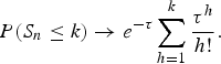
Indeed, S n = S n s is binomial with parameters (n,  (u n)), so that the result is just the Poisson limit for binomial distribution when n (u n) → τ.
We denote by M k,n the k-th maximum in the ordered sample of the maxima. Now, to evaluate the probability that P(M k,n ≤ u n) = P(S n ≤ k) we use Eq. (4) where the the explicit value for τ is taken as τ = −lnH θ. Indeed, by ordering the ensemble of maxima corresponding to the n s sub-cells,  denotes the order statistics of the sample (pattern), and we readily obtain from Eq. (4)

where Γn(x) = (n − 1)! e −x∑k=0n−1(x k/k!) is the incomplete Gamma function, and H θ(x) ≡ exp(−θexp(−x)) is the Gumbel (double exponential) law with the parameters a n = 1 (or a n → 1) and b n = ln n, and θ as the (clustering) shift parameter.
The joint distribution of several large maxima concerns the simultaneous exceedence of multiple hierarchic levels  by the sequence M 1,…M n s. Again, searching for the number S k n of the exceedences of the level u k,n s by the sequence, we obtain, see below, Eq. (6).
In fact, under the same hypothesis, it is possible to write down the joint law of the maxima between order 1 and k among the n s maxima, in decreasing order of intensity (Leadbetter, 1982, Reference Leadbetter1983; Embrechts et al., Reference Embrechts, Kluppelberg and Mikosch1997). With  and
 denoting k-th most intense maximum, and
 , following
 , one obtains for the joint probability for the k most intense maxima

Let us explicitely express the result of F (k)(x 1,…x k) for the first two maxima:

This allows us to evaluate the joint level of occurrence of the two most intense speckles, M n s,1 = M 1 and M n s,2 = M 2, which is the probability P[M n,1< M 1, M n,2 < M 2] ≡ F (2)(M 1, M 2), where of course M 1 ≥ M 2: Figure 1 shows the joint distribution for the two largest maxima,

expressing hence the (joint) probability that, at the same time, the most intense maximum is smaller than M 1, and that the second maximum is found below the value of M 2 (<M 1). We know that the marginal probability distribution for the second maximum F 2(M 2) is given by

which is a consequence of the fact that for sufficiently high values of M 1, say for M 1 > 2a n, the value of the most intense speckle is found most likely in the interval 0 < I < M 1. For this reason, the cut in Figure 1 (see also Fig. 2), at high M 1 values (M 1 ≃ 10 ≃ 2a n), approximately depicts the behavior of F 2(M 2).
(Color online) Joint distribution of the first two intensity maxima, M 1 > M 2, with ln n sp ≃ 5.29. Intensities are normalized to the mean intensity. The steepest gradient of the distribution in M 2 is asymptotically, for M 1≫ln n sp, found at M 2 = M 1 − ln 2 ≃ 4.6. (a) surface 3D graphics representation, (b): contours (in reduced interval).

(Color online) Derivative ∂M 2F (2)(M 1, M 2), with respect to M 2, of the joint distribution F (2)(M 1, M 2) of the first two intensity extrema, M 1 > M 2, corresponding to what is shown in Figure 1. Superposed to the contours is the curve following the steepest gradient of ∂M 2F (2).

Figure 3 shows the marginal probability density of the possible intensity values of several k-order maxima, which become more and more peaked (narrower) with order than the one for the most intense speckle.
(Color online) (a) Marginal probability distribution function, F(M k) and (b) the corresponding marginal probability density d F k/d M k of the 1st, 2nd, 3rd, and 5th (k = 1, 2, 3, and 5) most intense speckle as a function of their intensity M k. Dots display simulation results based on 1600 realisations of an RPP speckle pattern, the lines correpond to the model expressed by Eqs. (10) and (3). The simulation volume contains 2048 laser wavelengths in both directions, containing about n sp ≡ V foc/V sp = 1330 potential laser speckles such that the shift in the distribution is ln n sp ≃ 7.2.

2.3. Spacing in Intensity Between Maxima of Successive Order
The marginal probability for the k-order maximum (decreasing in intensity with increasing order) is equivalently the limit of Eq. (6) for all M 1 … M k−1 → ∞ (Embrechts et al., Reference Embrechts, Kluppelberg and Mikosch1997),

with x k = (M k − a n)/b n, which allows us to evaluate the distribution and the probability density of all higher order maxima as a function of their intensity,

In particular, by searching the expectation value in intensity,  k, with respect to the probability density of the k-th order maximum (Fig. 3)

with the function Ψ(k) standing for the Di-Gamma function (also call Poly-Gamma function of 0-th order and Γ(k) = k! for integers k). From this expression, one can determine the spacing  in M, given by the recursion identity Ψ(k) − Ψ(k + 1) = 1/k. Between the successive orders of speckle maxima, we have consequently the relation (in dimensionless units after normalization to the mean intensity of the overall speckle pattern <I >) k = 1 − ∑j=1k−11/j, which is 1 = ln n sp + γ (with γ ≃ 0.5772 being the Euler Gamma constant) for the principal maximum, k = 1. All higher orders, k > 1, can nicely be approximated by

with the expectation value of the most intense speckles of the order k = 2, 3 ,4, 5, and 6 yielding 2 = ln n sp + γ− 1 (≃ln n sp − 1/2), 3 = ln n sp + γ − 3/2 (≃ ln n sp − .94), 4 = ln n sp + γ− 11/6 (≃ ln n sp − 1.26), 5 = ln n sp + γ− 25/12 (≃ ln n sp − 1.51), 6 + ln n sp + γ− 137/60 (≃ ln n sp − 1.71), where the approximate values from Eq. (13) are given in the parentheses.
The spacing between the expectation values for first maxima is hence different from the spacing between the peak values, M k(peak), of d F k(M k)/dM k, which can be found from Embrechts et al. (Reference Embrechts, Kluppelberg and Mikosch1997) M k(peak) = ln n sp − ln k, (M k(peak) − M k−1(peak)) = ln[(k − 1)/k]. The histograms corresponding to either the peak or the expectation values can be written in the form

as illustrated in Figure 5. In comparison to the spacing of the expectation values k, the spacing of the peak values evidently yields an exponential decrease in the tail of the equivalent histogram f p(M k(peak)), whereas f e(k) has a slower decrease for the intense maxima and then comes close to an exponential one as well. This can be explained by the fact that the shape of the marginal probability densities (as a function of the speckle intensity) for the first order maxima is quite asymmetric around its peak, while for higher order maxima the shape becomes more and more symmetric. Figure 4 shows the comparison between peak values and expectation values as a function of the inverse of the speckle order, 1/k. In a similar way, we depict this difference between peak and expectation values in the form of an abundance histogram, indicating how many speckles, namely ≤k is equal to the order of speckle maxima k in average, with maximum intensity M being found in the interval M ≥ k.
(Color online) Dots: spacing between the expectation values for the intensity of the k-th order maximum, (k − k−1)/〈I〉 as a function of 1/k. Solid line: spacing between the peak values, (M (peak)k – M (peak)k−1)//〈I〉, of the probability density of maxima of successive order, following ln [(k + 1)/k], as a function of 1/k.

Histogram constructed by plotting the order k of the speckle maximum as a function of its peak (dotted line) and expectation values (dotted line with markers), M (peak) and k (from Eqs. (12) and (5)), respectively, as well as of the mean values in intensity (asterisks) for each speckle maximum from numerical simulations. Two series of simulations are shown with the corresponding values k ~ exp − M (peak) and k ≡ eq. (15), with (a) ln n sp = 8.3 (left group), and (b) ln n sp = 9.75 (right group). The simulations are based on about 1200 realisations of speckle patterns with identical optical properties, but different random distributions of the phase mask. The histogram corresponding to the peak values follows an exponential decrease ∝ e −M k, while the histogram corresponding to the expectation values and to the simulations follows a slower decrease in intensity according to Eqs. (12) and (15).

The histogram established via the numerical simulations shows very good agreement with the histogram, k = n spf e(k), where one associates the k-order maximum with its expectation value k in intensity, see Figure 5. We are therefore led to consider that the order of the maximum k determines, in an ensemble average over numerous realisations, the number of speckles with a peak intensity M greater or equal to the expectation value of the k-th order maximum, i.e., M ≥ k. (Note that the “peak intensity” of individual speckles M has to be distinguished from the “peak value” M k(peak)) of the marginal probability density of the k-th order maximum). We can hence use the inverse of Eq. (12),

represented in Figure 5. This equivalence allows us, hence, to use Eq. (5) as an expression for the “tail” of the distribution for high-intensity speckle maxima. The fact that we start counting, due to the order statistics, from the most intense speckle toward the less intense ones, has the consequence that the “body” of the speckle maxima distribution corresponds to very high orders k ~ e −1n sp.
2.4. Computing the Response from Independent Speckles
In the frame of the “independent hot spot model” (Rose & DuBois, Reference Rose and DuBois1994), it is of interest to compute response of a speckle (or “hot spot”) pattern to a nonlinear physical process. For the purpose, to compute the response  to such a process from the ensemble of speckles in a plasma, the assumption of independent “hot spots” means that one can sum over the contributions to the response from each speckle,
 , i.e.,
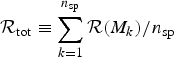 , where the response of the speckles (numbered from k = 1 to n sp) is a function of the speckle peak intensity M k. The validity criteria for such an approach are (1) that the process considered (e.g., stimulated scattering) can be expressed by either a stationary or an instantaneous response function, and (2) that the contributions of adjacent layers in the speckle pattern do not give rise to subsequent re-amplification. In practice, this means for the case of stimulated scattering in speckles, that the light scattered off different layers with respect to the laser propagation, originating from the (sub-) ensemble of speckles in each layer, can be considered as an incoherent superposition of the individual contributions.
We shall consider the particular case of stimulated scattering, for which the above mentioned criteria can be explicited for an inhomogeneous plasma (Tikhonchuk, 1997): (1) the stimulated scattering process is in a convective amplification regime where the plasma waves, off which electromagnetic wave are scattered, are strongly damped; (2) the plasma is inhomogeneous with a three-wave-coupling interaction length ℓint that is shorter than the longitudinal speckle length 2l z (see Appendix B), but longer than the speckle width 2l ⊥. For a plasma wave damping rate νa/ωa and a plasma inhomogeneity length L ∇, the latter condition can be expressed by 2l ⊥ < ℓint = (νa/ωa)L ∇ < 2l z.
For a layer of the length of a speckle, ~2l z (see Appendix B for the equivalence between l z, the Rayleigh length, and the length  ), the response function for the backscattered light flux produced due to parametric scattering instabilities, such as stimulated Brillouin and raman scattering (SBS and SRS, respectively), can be written as
 . With R sp( ) we denote the single speckle reflectivity, i.e., the portion of light—with respect to the incident light flux—that is backscattered off a single speckle. A speckle having M k times the mean intensity 〈I〉 of the incident beam, contributes hence with R sp (M k) M k to the total backscatter response.
Following the above-mentioned argument that the contributions of adjacent layers of the length of a speckle do not give rise to re-amplification, the total backscatter response can be expressed consequently by the double sum

where n sp, j denotes the number of speckles in each of the j z = [L foc/2l z] layers of length 2l z, and where the contribution from each of the n sp,j speckles, M k jR sp(M k j), is evaluated in the j-th sub-layer around z = z j with 0 < j = [z j/2l z] < L foc/2l z. The sub-division into sub-layers is necessary in case that the response in each of the j z layers depends on the local plasma quantities like density, damping etc., and/or in case of pump depletion of the local laser power (see model in Tikhonchuk et al., Reference Tikhonchuk, Hüller and Mounaix1997) such that 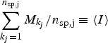 is no longer constant, but diminishes along the propagation axis.
Under the condition that the spatial dependence of the local contributions on z is negligible, so that R sp(M k,j) does not considerably vary over L foc along the propagation axis, this expression simplifies to

for the entire speckle pattern with n sp = ∑jn sp,j. In this sum, the order of the contributing speckles does not matter. In the ensemble average over many realizations, one can use the values of the successive orders k in intensity of the speckle maxima M k, as developed above.
For a single realization of a speckle pattern, as for a concrete speckle pattern, Eq. (16) can easily be determined. In many cases, only the optical properties of a speckle pattern are known, but not the details of the pattern, and therefore a single realization is statistically not representative for the high-intensity tail of the speckle distribution. For the ensemble average over many realizations of speckle patterns, the computation of the response requires an integration over the joint probability distributions F (k)(M 1 … M k), which is pratically a very tough procedure. We can, however, make use of the quite general feature seen in Figure 2: for the example of the joint probability density for M 1 and M 2, it can be seen that the joint probability density in M k+1 already tends, as a function of M k quite rapidly toward its asymptotic form corresponding to the marginal probability density.
For this reason, the model developed in Section 2.3 can yield a good estimate of Eq. (16) by evaluating R sp(M k) at the expectation value k of the k-th maximum, yielding

The latter is a good approximation provided that the change of the response function R sp in the interval around M k = k determined by the variance σk of the marginal probability density Eq. (11), namely  , is small compared to R sp(k).
Using Eq. (12), the sum applies to discrete values of k. In contrast to our discrete approach, the distribution of speckle maxima as a function of their peak intensities has been expressed by a continuous expression (Garnier, Reference Garnier1999). It might therefore be useful to express the sum of Eq. (17) in the form of an integral

with df e(M) ≡ (df e(M)/dM) dM, knowing that 
 . This approximation is, however, not very precise for orders k < 3, because we took interpolated values when performing the partial integration. The latter expression yields, in the continuous limit,
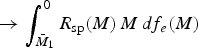 . We can here use the fact that the values of k can be approximated in a continuous manner, using Eq. (13), such that the inversion of Eq. (5) readily yields a nice approximate explicit expression of the speckle maxima abundance f e(k), namely with the function

which is normalized to the total number of speckle maxima, namely n s = n sp = exp{a n} = exp{ln n sp}.
2.5. Numerical Simulations of Order Statistics
We have performed numerical simulations in order to determine the order statistics from speckle patterns generated by a RPP. For this purpose, we have solved the stationary paraxial equation for a forward-going laser pulse

where the wave number k 0 and and the frequency ω are chosen such that ω2/c 2 − k 02 ≡ 0, because of the dispersion in a homogeneous medium or vacuum. The corresponding solution of a light field composed by speckles can be written as the superposition of an ensemble of complex fields a m, all with the same propagator e ik 0ζ−iωt, but with distinct values in the transverse direction. The field describes, in paraxial approximation, the propagation from the so-called “near field,” where the speckle-generating RPP is situated, ∑ma me iφm, toward the “far field” E(x, z) in the focal plane. How concrete realizations of RPP beams can be done is explained in more detail in Appendix B.
Our simulations are performed on a highly resolved mesh over a large lateral size and over many characteristic lengths, namely Rayleigh lengths of speckles in the propagation direction, with typical number of speckles of 2000, thus ln n sp ~ 7.5. The total number of mesh points (8 to 16 × 1016) is considerably higher than n sp such that a great number of points inside a speckle are clustered and the shift ln n sp on the intensity axis applies. From the simulations we have determined the most intense speckle maxima, starting with M 1, up to order 6 in the case presented here. To determine the highest intensity value M 1, being a local maximum at the same time, follows a straightforward procedure. The next maxima following in order, M n < M n−1 < … M 3 < M 2 < M 1 have to be determined with caution because the error in ordering the maxima increases with the order. The algorithm chosen may therefore modify considerably the result. We have therefore devoted Appendix A to explain the searching procedure for the maxima. Let us just mention that the most efficient method is to divide the volume in sub-cells of the size of a individual speckle, in respecting the typical sizes due to the manner how the speckle pattern is generated with the RPP. For the different cases of RPP masks in the “near field,” we have listed the specific speckle volume in Table 1. The maximum of each sub-cell is retained, and all maxima are sorted in magnitude, however, to reduce errors, a discriminating filter can be applied, see Appendix A. In order to establish the probability distribution numerically, we have computed a large number of realizations of RPP masks with identical optical properties: that means that the focusing optics, the size of the overall phase plate, and the size of the phase plate elements is the same in each realization, whereas the phase shift φm(j) in each individual element m follows a random value sequence from realization j to realization j + 1. It is unimportant whether φm(j) randomly jumps between the values 0 and π/2 or whether the values of φm(j) have homogeneous distribution in the interval (0,π/2). The order statistics can be determined in registering the intensity values of the first k (here 6) most intense maxima. Numerically determined probability distributions for extreme speckles are shown in Figure 5. From the same statistics we have determined the expectation value of the k-th order maximum, which is compared to the values derived from probability theory in Eqs. (13) and (19) above. Both comparisons shown in Figures 5 and 4 show very good agreement between simulations and theory. In Figure 4, the spacing between the expectation values for the successive maxima clearly exhibits a departure from the 1/k law for small k, i.e., for the most intense speckles, giving rise to a simply exponential (exp − M/〈I〉) speckle distribution. The histogram, see Figure 5, counting the number of maxima in the interval M < M k, which represents the upper tail of the speckle distribution, shows hence a decrease that is slower than an exponential for the maxima below order 8, namely for M > 8 ≃ 3〈I〉.
3. BACKSCATTERING FROM EXTREME SPECKLES
Let us show the pertinence of the order statistics developed above for the example of the backscatter reflectivity value of a parametric instability. We will illustrate it for the particular example of SBS by making use of simulation results from the Harmony interaction code (Hüller et al., Reference Hüller, Masson-Laborde, Pesme, Casanova, Detering and Maximov2006) for several realizations of a speckle pattern generated with a RPP. The simulations were carried out in an inhomogeneous plasma with a linear velocity gradient of an exploiding-foil type plasma such that SBS in single speckles should follow that amplification according to Rosenbluth's model (Rosenbluth, Reference Rosenbluth1973). Ion acoustic waves are assumed to be strongly damped.
To compute the SBS reflectivity from the model developed here, we can assume that the contribution to backscattering comes independently from each speckle. The reflectivity can be compute by summing over all speckles with a response function of the reflectivity R(M k) parametrized on the speckle peak intensity M k, as done, e.g., in Hüller et al., Reference Hüller, Mounaix and Tikhonchuk1998 and Tikhonchuk et al., Reference Tikhonchuk, Hüller and Mounaix1997, following an amplification described by Rosenbluth's model (Rosenbluth, Reference Rosenbluth1973). For a concrete speckle pattern, the values of the speckle maxima M k are known. One can hence compute the reflectivity  corresponding to backscattering of the overall speckle pattern by
 from Eq. (17), for all M k being normalized to the mean intensity 〈I〉. The value R(M k) indicates, as mentioned earlier, the fraction of light flux that has been backscattered off an individual speckle. One can assume that the single speckle reflectivity is a result of an exponential amplification with R sp (M) ∝R noiseexp{GM} from a noise level R noise, with G being the SBS gain for an average-intensity speckle, and M standing for the peak intensity value of an individual speckle. For simplicity, here, we limit the single speckle reflectivity by unity once the speckle peak intensity M k exceeds the value of ln(1/R noise)/G. We readily obtain

which can be further evaluated using the approximate expression Eq. (13) for the expectation value k of the succesive orders of the speckle maxima,

It is important to note that, starting from the general expressions (Eq. (17) and (21)), the contribution of the most intense speckles to the total reflectivity R tot yields a non-negligible portion. For the case of a realization yielding a particular pronounced principal maximum such that difference between the first two maxima 1 − 2 is considerably larger that the successive differences k − k−1, the contribution of the principal maximum to  can assume a high percentage.
Figure 6 shows the simulation results for the SBS reflectivity of a speckle pattern with about n sp ~ 1820 speckles. The SBS gain corresponding to these simulation yields for average intensity speckles at 〈I〉 the value of G = 1.1, the noise in the simulations was such that an average reflectivity of R noise ~ 10−5 results in absence of amplification (i.e., for G = 0). Since the gain for an average-intensity speckle (at 〈I〉) is small, only intense speckles can contribute to  . For this reason, each different realization of simulations reaches eventually a different reflectivity level, plotted here as a function of the principal intensity maximum M 1. The dependence of the reflectivity on M 1 brings to evidence the fact that the contribution of the most intense speckles, and their fluctuations in intensity, cannot be neglected if the number of speckles is limited.
Backscatter reflectivity of Stimulated Brillouin Scattering, computed from different realizations of a speckle pattern generated by a RPP. Each point corresponds to a realization for which the reflecitivity is plotted as a function of the peak intensity M 1 in the respective speckle pattern. Simulation parameters: average beam laser intensity 〈I〉 = 2 1014 W/cm2 at the wavelength λ = 1 µm, electron temperature T e = 1 keV, and density n e = 0.1n c, ion wave damping νa/ωa = 0.1, velocity profile inhomogeneity length L ∇v = 150λ, optical f-number f # = 5 resulting in a specific speckle volume of 2l z, RPP × 2l⊥, RPP ≃ 175λ × 4.2λ (see Table 3 of Appendix B for “modified flat top”), and plasma volume L z × L x ⊥ = 500λ × 717λ, equivalent to ln n sp ≃ 6.2.

The evaluation of the average SBS reflectivity corresponds to an ensemble average of many realisations of speckle patterns with each time n sp speckles. Applying Eq. (23) for the current example, this yields a value of R tot ≃ 0.0003. The histogram in Figure 6 shows that the reflectivity assumes this value around the expectation value of the most intense speckle, namely 1 = ln n sp + .5772, being 1 ≃ 8.1 for n sp ≃ 1820, hence in good agreement with the average over the realisations in our simulations.
We have compared our results to previous work on the statistics on speckle maxima, which is shown in Figure 7. In addition to the speckle maxima histogram f e(k) corresponding to our model, see Eqs. (15) and Eqs. (19), we show the corresponding distribution from work done by Garnier (Reference Garnier1999) where f G(M) has a powerlaw-type times exponential dependence in M, f G(M) ~ n sp (c 1M d/2 + c 2M −1+d/2) exp (−M) with c 2 = π/2 + 1 and c 2 = 1 in 2 spatial dimensions, d = 2, and c 1 = 1 and c 2 = −3/10 in 3 spatial dimensions, d = 3. To understand the impact of the differences between the PDFs for f e(k) and f G(M), we have furthermore computed the mean backscatter reflecitivity, as explained above, both from Eq. (refrmean) and by convolving the PDF ∝ f G(M) with the single speckle reflectivity parametrized by the gain value G (of an average-intensity speckle),

here with a noise level R noise = 10−5, and again with df G ≡ (df G/dM)dM. Note that, for practical reasons, the integral is truncated at the lower bound of the mean intensity of the beam (M ≡ 1) because (1), for not too high gain values, speckles with lower intensities do not potentially contribute, and because (2) the speckle maxima distributions, both f e and f G, are usually poorly reliable for lower values, which is a consequence of the fact that a low intensities (with respect to the mean beam intensity), speckles can hardly be distinguished from each other. Let us remark that in the shown example, the gain is entirely proportional to the average (speckle) intensity. The gain can also be changed by varying the speckle size (not the case in our simulations), which would, however, for the same overall volume, change the number of speckles. This has to be taken into account when using Eq. (23).
(Color online) (a) Comparison between the speckle maxima probability distribution computed from Eq. (19) (solid line) and Garnier's results (dashed line) (Garnier, Reference Garnier1999). (b) Mean backscatter reflectivity computed from Eqs. (19) and (21) (solid line) and from Garnier's model (dashed line) with a single speckle reflectivity parametrized with R sp (M k) = min{1, R noise exp(G M k)}. The isolated points show the reflectivity corresponding to simulation results with the code Harmony. The multiple values displayed by points at G = 1.1 correspond to the range of values displayed in Figure 6 for several realisations with the same parameters.

In the past, the speckle maxima distributions due to work by Rose and DuBois (Reference Rose and Dubois1993) and Garnier (Reference Garnier1999) have shown to yield good agreement with numerical simulations (Hüller et al., Reference Hüller, Mounaix and Tikhonchuk1998). In what concerns the regime illustrated here, we observe that for sufficiently high gain, say G ≥ 2, the comparison of our and Garnier's results do not show a particular difference, while the difference is striking for relatively small values 0.3 < G < 2. In particular, our simulation result, which yields an ensemble average reflectivity 〈R〉 ~ 0.0003, is well reproduced by our model computed with Eq. (23). Note that for the shown case, with the number of speckles of the order of ~2000, the most intense speckles will have intensities around eight times the mean intensity, with statistical fluctuations around this value, as illustrated in Figure 6. The variation of the average reflecitivity is hence non-negligible, as indicated by an error bar for the value of G = 1.1 in Figure 7b. Following Garnier's PDF using Eq. (23), equivalent to Eq. (23) for a continuous expression f G(M), the ensemble average reflectivities yield values for 0.7 < G < 2 that are almost by one order of magnitude higher than those of the simulations, thus fairly outside the interval indicated by the error bar.
Just in the mentioned interval of gain, 0.5 < G < 2, the contribution of the (about) 10 most intense speckles to the average reflectivity is of the order of 20% or higher, so that the order statistics of intense speckles, have a strong impact, see Figure 8. At high gain values, the main contribution to the reflectivity is evidently dominated by the numerous speckles in the “body” of the speckle distribution function, usually well-described in previous work (Rose & DuBois, Reference Rose and DuBois1993; Garnier, Reference Garnier1999). Differences in models describing the tail of the speckle distribution function should not be too important in this high-gain regime. In the moderate- and low-gain regime, G ≤ 1, however, a good description of the tail in the speckle maxima distribution is necessary, provided that the gain in the most intense speckles, G k = G k with, say, 1 ≤ k < 20, is sufficiently high, say G 1 ~ ln n spln (1/R noise).
(Color online) Proportion of the sum of backscatter reflectivities from the speckles up to the K-th order to the total reflectivity R tot of all speckles, corresponding to the above-mentioned cases, for three different gain values G = 1.1 (blue dots, intermediate), G = 2 (red dots, upper curve), and G = 3 (green dots, lower curve).

4. DISCUSSION AND CONCLUSIONS
With the help of the theory of extrema, we have derived the order statistics of intense laser speckles in a laser beam generated by RPP. The distribution function for each of the most intense laser speckles, conditioned by the order k of occurence in peak intensity M k in speckle patterns, has been derived from the joint probability distribution F (k)(M 1,…, M k) over k(≥) speckle maxima. The theoretical result is in very good agreement with numerical simulations over numerous realisations of speckle patterns. To establish the order statistics from these simulations, a selection procedure has been applied that is based on the sub-division of the simulation volume in sub-cells having the characteristic size of individual speckles. In a further step, we have established the histogram f e(k) for the high-intensity tail of all speckle maxima via the expectation value in intensity of each order k derived from the marginal probability density, dF k(M k)/dM k, for each speckle maximum.
For the example of SBS from a speckle pattern in the regime where the contribution from “independent” speckles can be approximated by a sum, we have compared our model with numerical simulations, revealing good agreement. The comparison underlines as well that particular importance to the precision of the description in the high-intensity tail of the speckle distribution function has to be given. The fact that our approach is accentuated to this regime, it allows to compute, with higher precision than available from previous work, the contribution from intense speckles to critical nonlinear processes.
In experiments with relevance to laser fusion, the influence of high-intensity speckles is not at all desired. Therefore laser beams are designed to contain as much as ~105 speckles. It is furthermore evident that the experimental parameters have been designed such that speckles that have peak intensities of 2–5 times the mean intensity, should dominate essentially most of the physics processes, as far as they can be entirely controlled. On the other hand, experiments that have been performed with a relatively “small” number of, say ≪104, speckles in the plasma volume, may require a more precise analysis of the speckle distribution, as provided by our model, because the onset of potentially nonlinear processes may be energetically important under such circumstances. Furthermore, processsus with threshold-like behavior for the onset of absolute instabilities, or of laser-beam self-focusing, might be particularly sensitive to the distribution of speckles in the high-intensity tail (even though saturation of such processes may limit their importance).
The theory developed here is based on the assumption of an idealized speckle pattern generated by RPP beams. This means that at least speckles with peak intensities higher than the average intensity of the beam, 〈I〉, can all be characterized by the same characteristic sizes along ( ) and across (ℓ⊥) the laser propagation direction. For speckle patterns generated by the superposition of optically smoothed laser beams, these characteristic sizes can be described by a probability distribution, namely F(
 ), where
 can be either independent of, or coupled to the value of
 . The latter is the case for RPP beams (with
 ).
Nonlinear response of processes like self-focusing in intense speckles, as well as pump-depletion due to strong scattering in speckles, can considerably change the image of the speckle pattern inside the plasma. This is not taken into account in the present work. A calculation including the nonlinear modification of the speckle pattern in a plasma has to be done for such purposes, which can hardly give a universal response to the potentially arising mechanisms. Numerical simulations can partially give an answer to this problem. Starting from simulations, statitics of so-called “plasma-induced smoothing” of laser beams have already been investigated (Hüller, Reference Hüller2003) for the case of “dancing filaments” (Schmitt & Afeyan, Reference Schmitt and Afeyan1998).
To establish the order statistics of speckle patterns with multiple characteristic lengths, or with a statistical distribution of characteristics lengths, ℓ⊥ and  , it is more appropriate to consider boxes of different sizes. Therefore, as above, one has to proceed in the way that the focal volume, containing the speckle pattern, is evaluated at n mesh points, and is sub-divided in n s sub-cells. Each cell contains the number of n k points, for which holds ∑kn k ≤ n. We can still consider that the maxima of the sub-cells are independent, and being distributed following the Gumbel law with the shift parameter θk, if (1) each sub-cell contains in the limit of a very large number of points n k, say n → ∞, and if (2) the sub-cells are disjoint and sufficiently separated for large values of n. Then θk is found from the limit law of a sequences of “clustering” intensities (exponential law) for the fraction of points observed in the k-th sub-cells.
The fact that the superposition of optically smoothed laser beams gives rise to non-homogeneous speckle sizes (characterized by a statistical distribution of them), may lead to a modulation of the limit law for the most intense maxima. This is subject of work in progress.
ACKNOWLEDGMENTS
We wish to thank Ph. Mounaix and B. B. Afeyan for helpful discussions. This work has been partially supported by the Agence Nationale de Recherche, project title “CORPARIN” no. ANR-07-BLAN-0004. Simulations have been performed thanks to access to the computing center IDRIS-CNRS.
APPENDIX A: CHOICE OF SPECKLE MAXIMA IN SUB-CELLS
In order to find an adequate selection procedure for the speckle maxima by sub-division in cells, various problems have to be handled: (1) First of all, the characteristic size of speckles has be chosen adequately, which can be done with the help of the lengths listed in Appendix B, and the specific speckle volume listed in Table 1. An inadequate choice may increase the error in the order statistics with increasing order of the maxima. (2) To locate the sub-cells in the simulation volume, there are essentially two main choices for uniform size cells: (i) the cells regularly are placed in adjacent order starting from one corner of the simulation volume, or (ii) all cells are placed around the cell containing, in its center the principal maximum of the speckle pattern. Once the volume is sub-divided in n sp sub-cells, it is straightforward to determine the principal maximum of each. The resulting n sp values found can be ordered in decreasing order. However, subsidiary of intense maxima that drop into a neighboring cell, because of the vicinity of the principal speckle peak to a cell border. Such subsidiary maxima that may exists depending on the generating method (“flat-top” or “Gaussian,” see Appendix B), are a consequence of the coherent structure inside speckles. They can be considered erroneously as the real peak maximum of the cell and hence falsify the order statistics. Method (ii) avoids this error for the case of the most intense speckle of the entire volume. However, beyond this order, the confusion persists between subsidiary maxima, that are correlated to the main speckle peak, and the real peak value of another speckle. For this reason, a second selection step is necessary: after having established the order between the maxima, all of those ones are eliminated, which are too close to an intenser maximum in a neighboring cell. In practical terms, one can define a distance that should not fall below a length of the order of  and/or
 (see herefore Appendix B). It is preferable to eliminate realisations that are subject to error.
Following the same arguments as in Leadbetter (1982, Reference Leadbetter1983), which we apply to random variables representing speckle intensities, the location and the height of the speckle peaks can be considered as being independent of each other; furthermore, the distribution of the location is uniform, so that we expect that method (i) and (ii) for the choice of subcells give the same results (despite small errors due to problems evoked in 2) provided that simulations are based on a sufficiently high number of realizations and points in space. Nevertheless, for a reasonable choice of simulations, it appears that numerical results for the cells according to method (ii) are the best with respect to our model results.
APPENDIX B: A GUIDE FOR MODELLING SINGLE UND MULTIPLE LASER SPECKLES IN 2D AND 3D
A Gaussian laser beam can be defined by its electric field according to the paraxial solution in the space dimensions ξ along and x ⊥ across the propagation direction

with the width of the beam

at the distance ξ from the focus, involving the width at best focus w and the definition of the Rayleigh length L R. In 2D, we have f 2D(ξ) = W(ξ)−1/2 being a function decreasing slowlier with the distance ξ = z − z 0 in the focal point at z 0 than in 3D (cylindrical) geometry, for which the decrease f 3D(ξ) = W(ξ)−1 to 2−1/2 occurs a the one Rayleigh length ξ = L R. It is important to note that the integrals over the square amplitudes differ decisively from 2D to 3D, namely the integral does not converge in 2D, while the integral converges rapidly in 3D geometry,

for L → ∞.
In the so-called “near field image,” which is principally the Fourier transform of the field in the focal plane (usually called “far field”), we can write the field as

where the function Q(k ⊥) is also a (1) Gaussian Q(k ⊥) ∝ exp(−4 w 2k ⊥2)] for the Gaussian field Eq. (24), and a so-called, (2) “flat-top” for

For both cases, in 2D, the integrals over z in the square amplitude diverge. To remedy the problem of the missing convergence of this integral in 2D, Rose (Reference Rose1997) has suggested a beam called (3) “modified flat-top” by using a function  for
 , and 0 elsewhere. This yields the following shape around the focal point,

which has a converging integral along z.
The cutoff value q of the “flat-top” beams in the transverse wave vector determines the width ∝q −1 in of the beam in the focal plane. In 3D, the shape along the propagation axis (for x ⊥ = 0) is given by

being identical to the one of the cylindrical flat-top speckle, for which the amplitude for z = 0 is given by

For both types of beams, the modified flat-top in 2D and the cylindrical flat-top in 3D, due to the identical behavior in z, the integral 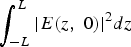 converges for L → ∞ to the same value πq.
For the ordinary “flat-top” speckle, (2), in 2D (i.e., a single transverse dimension), generated by Q(k ⊥) = const in Eq. (25), the shape of the field in the 2D space spanned by the coordinates (x ⊥, z) is hence, along each axes, given by

and

being equivalent to the behaviour of a Fresnel integral as a function of z. From these shapes, we henceforth deduce characteristic lengths, indicating the measure of a typical size of the beams, which eventually allows to determine the specific speckle volume.
In Table 2 we indicate the correlation lengths with respect to the transverse x ⊥ and the longitudinal dimension z, for which we use the following definitions  and
 , used in the tables below. Alternatively, by defining the widths l ⊥ (in x ⊥ or r) and the lengths l z by the distance where the speckle intensity assumes one half of the peak value, one obtains the values (by using a = 2−1/2w) as listed in Tab. 2.
Summary of typical longitudinal and transversal sizes of a single speckle, generated by different methods in the near field

Summary of typical longitudinal and transversal sizes of speckles in a RPP pattern, generated by different methods in the near field

B.1 Case of the equivalent RPP beams
Equivalent to the above definitions one can determine the corresponding beam features when a Random Phase Plate is introduced in the beam path before the focusing lens (Rose & DuBois, 1993b)

where ϕk jumps randomly between the values 0 and π in the intervals in k ⊥. One can evaluate the shape of individual speckles in the focal plane without knowing the explicit distribution of the ϕk-values, with the help of the auto-correlation function defined as

For the particular case of the “modidied flat-top” with a RPP one obtains, we can again use Eq. (25) but with a amplitude function, now going with the square root of the perpendicular wave vector, Q RPP(k ⊥) = | k ⊥/q|1/2 for |k ⊥| < q which is different from the coherent case, (3), discussed above. The expression for the 2D standard flat top, the cylindrical flat top and the Gaussian are immediate from the above definition 28 and are not explicited here.
We list in the following the typical lengths and widths of speckles generated by a RPP corresponding to the generating “near-field” configuration. The corresponding values for the specific volume occupied by a speckle are listed in Table 1 found in the main text. The latter is of particular importance to determine the number of potential speckles in a finite focal volume.
To have equivalence between Gaussian and flat-top description, the following condition has to be satisfied (Rose & DuBois, Reference Rose and DuBois1993) q = k 0/2 f # = π/(f # λ0) yielding in 2D: w RPP2D ≃ 2.1(1.95)/q ≃ 0.64f # λ0 between Gaussian and flat-top (modified flat-top); in 3D: w RPP2D ≃ 2.65/q ≃ 0.84f # λ0.



