Economic historians and macroeconomists have documented in great detail the aggregate behavior of the U.S. economy during the Great Depression. However, much less is known about the distributional consequences of the downturn. Work going back to Kuznets (Reference Kuznets1953), Goldsmith et al. (Reference Goldsmith, Jaszi, Kaitz and Liebenberg1954), and Tucker (Reference Tucker1938) has attempted to measure changes in the distribution of income and to identify which sectors, regions, and individuals were most affected by this unprecedented event. Measuring and explaining these distributional changes is important not just in determining who bore the cost of this event but also for understanding the aggregate dynamics themselves. As Robert Margo (1993, p. 41) wrote, “[D]isaggregation [can reveal] aspects of economic behavior hidden in the time series[.]” For example, a central controversy surrounding the labor market is why real wages were “sticky” in the face of unprecedented levels of unemployment. Solving this puzzle requires understanding the wage-setting behavior of workers and businesses at a disaggregated level. A major problem for economists wanting to take this disaggregated approached has been fragmentary data sources.
Our first contribution is to fill in this gap in the data sources available by constructing an establishment-level dataset consisting of 25 industries from the Census of Manufactures (COM) between 1929 and 1935. We use this dataset to study the effects of the Depression on the distribution of earnings per worker. Our dataset allows us to confirm earlier work that used data disaggregated to the industry (Bernanke and Powell 1986) or regional level (Rosenbloom and Sundstrom 1999). However, we can go beyond earlier work to address questions such as the role of establishment entry and exit on the earnings distribution that is not possible with existing sources. Our dataset, while not covering all of manufacturing, is representative of this sector along many dimensions: geographic, types of products, and scale of production. For each establishment, we observe the earnings of wage earners and of salaried workers, which we refer to as blue- and white-collar workers.Footnote 1 From this, we measure earnings per worker for each skill group.Footnote 2
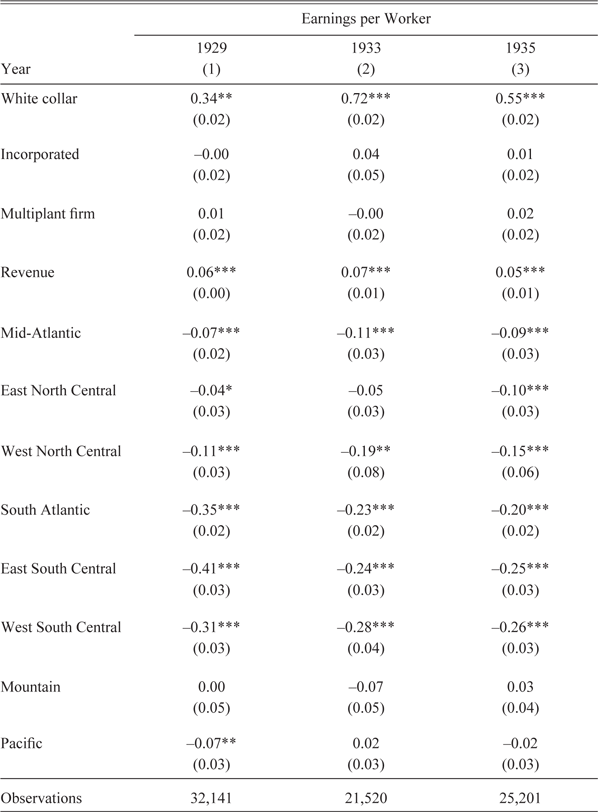
We first characterize the distribution of establishment-level earnings per worker and the observable factors that affect this distribution. Both the differences between the 75th and 25th percentiles and between the 90th and 10th percentiles decline from 1929 to 1933 by around 10 log points. While the 75–25 difference subsequently returns to its 1929 level by 1935, these changes are driven by shrinking gaps between the bottom and median of the distribution offsetting widening gaps between the top of the earnings distribution and the median. In particular, the 90–50 difference increases by 22 log points between 1929 and 1933 before falling 25 log points between 1933 and 1935. Conversely, the 50–10 difference declines 30 log points between 1929 and 1933 before increasing 10 log points between 1933 and 1935. The changes in the overall earnings distribution are almost totally driven by the changes in the blue-collar earnings distribution since the white-collar distribution shows very little change. We next use the decomposition of Juhn, Murphy, and Pierce (JMP) (1993) to account for the changes in the earnings per worker distribution by decomposing the changes into changes in observables, returns to those observables, and unobservables. Changes in the distribution of observables, if anything, act to increase inequality over time, but the magnitude relative to the overall change is quite small. At the same time, changes in the unobservable component play no role over time. Instead, the initial compression in earnings across establishments is driven almost entirely by changes in returns to observables, in particular, regional differences. For example, in the East South Central region, on average, earnings per worker are 41 log points below those in New England in 1929, 24 points lower in 1933, and 25 points lower in 1935, confirming some of the results from Rosenbloom and Sundstrom (1999). On the other hand, changes in the skill premium work in the opposite direction, widening inequality. After controlling for observable establishment characteristics, the gap between earnings per blue- and white-collar worker increases from 34 log points in 1929 to 72 log points in 1933 before declining to 55 log points in 1935.
This latter result qualifies our understanding of the remarkable compression in earnings by skill over the first half of the twentieth century (Goldin and Margo, 1992).Footnote 3 While the patterns in the skill premium we find match those of clerk wages relative to unskilled weekly wages (see their Figure II), we find less evidence to support their claim that “inequality narrowed after 1933, probably because of the minimum wages of the National Industrial Recovery Act” for the simple reason that, for blue-collar employees, the 75–25 differential increased between 1933 to 1935 and the 90–10 differential barely changed. Wright (Reference Wright1997, p. 214) also points to the role of minimum wage particularly in explaining the convergence of the South. However, we find that the convergence happens before 1933, when the minimum wages were implemented in the New Deal. In fact, our results are exactly what would be expected if, as Goldin and Margo claim, “unemployment … was disproportionately borne by the least educated and lesser skilled,” and as the economy recovered from its trough in 1933, less productive and, hence, lower paid workers were hired back.
In light of Goldin and Margo’s claim about the importance of selection, we study the effects of entry and exit of establishments on the evolution of the earnings distribution. This explanation of changes in inequality is connected to one explanation of why real wages were sticky in the Great Depression, and in recessions more generally. That is, the apparent stickiness is an artifact of aggregation (Stockman Reference Stockman1983). This theory posits that the first workers to be fired or to have their hours cut in a recession are the least productive and, hence, paid the least. Furthermore, these workers are the last to be hired back as the economy recovers. All else equal, this shift in the composition of worker quality would lead to a countercyclical aggregate real wage masking procyclical real wages at the level of the worker.Footnote 4 Direct empirical evidence for this theory for the Great Depression is rather limited. Margo (Reference Margo1991, p. 333) finds that the newly unemployed were “drawn disproportionately from the low-wage portion of the labor force,” but this is based on one-time surveys in Buffalo in 1929 and 1930, as well as Michigan and Philadelphia in 1935, and the 1940 Census of Population. In addition, Margo (1993), citing a paper by Lebergott (Reference Lebergott1989), claims that workers who were laid off were less productive and paid less.
While we cannot observe this selection process at the level of the worker, we can examine selection at the establishment-level and the extent to which higher or lower paying establishments differentially exited or entered. We find that, in fact, white-collar workers at both newly entered and exiting establishments had lower earnings of between 3 and 14 log points, depending on the year and specification, than those at continuing establishments. The same penalty is generally present for blue-collar workers at exiting and entered establishments, but overall, these differences are much smaller in magnitude. These findings complement existing work that has studied the role of productivity in determining exit of establishments during the Depression (Bresnahan and Raff 1991; Scott and Ziebarth 2013; Lee Reference Lee2014).
To quantify the effects of entry and exit on changes in inequality, we construct two counterfactuals. The first predicts what earnings per worker would have been for exiting establishments if they had not exited based on changes in earnings of establishments with similar characteristics that did not exit. We calculate inequality measures for this counterfactual earnings distribution, including the continuing establishments and imputed values for the exiting ones. We find that the 75–25 and 90–10 differentials of the exit counterfactual distribution for blue-collar workers are 6 log points higher in 1933, which would explain about one-third of the decline in those statistics over the same period, and are negligibly different in 1935. The second counterfactual simply removes the penalty associated with newly entered establishments in a given year. The counterfactual distribution here is only marginally different than the actual distribution across all years and skill classes. These results show that the exit margin played an important role in the decline in inequality over the first half of the Depression, consistent with a version of Goldin and Margo’s claim and the aggregation bias explanation of sticky wages. However, this effect was asymmetric, with exit playing a very small role in the rise in inequality between 1933 and 1935.
While there are clear strengths of our dataset, it is important to keep in mind its limitations for extrapolating to the overall earnings distribution. First, we lack information on those not employed in manufacturing. Employment in manufacturing only comprised about one-third of total non-farm employment in 1929, but, because of the sharp declines in manufacturing employment between 1929 and 1933, the declines in this industry explain about 43 percent of the total decline in non-farm employment. This makes it particularly important to study manufacturing for understanding the Depression, and its importance is reflected in the long literature that focuses on this sector of the economy (Bernanke Reference Bernanke1986; Bernanke and Parkinson 1991; Bresnahan and Raff 1991; Rosenbloom and Sundstrom 1999). The second limitation is that the changes in the earnings distribution we measure are for the employed. The Great Depression saw a large increase in unemployment, from just over 3 percent in 1929 to a peak of 22.6 percent in 1932 (Darby Reference Darby1978). The earnings of workers who were formerly employed in manufacturing and became unemployed or employed in a different sector are not captured by our sample.
A final limitation is that, with few exceptions, the literature on inequality has used data drawn from household surveys to estimate earnings inequality at the worker level, while we use establishment-level data. The resulting measures of inequality are distinct and the comparison between our results and those in the literature using worker data is a bit more difficult. At the same time, our approach is consistent with a new literature that has emphasized the importance of demand-side factors in determining inequality (Card, Heining, and Kline Reference Card, Heining and Kline2013; Barth et al. Reference Barth, Alex Bryson and Freeman2016; Song et al. Reference Song, David, Guvenen, Bloom and von Wachter2019). This new view that emphasizes firm and establishment characteristics should be contrasted with the older, supply-side view that emphasized worker characteristics such as education or experience. Though our use of labor demand-side information is partially motivated by data availability, our results, particularly those focused on the extensive margin, highlight the importance of this side of the labor market.
There is an existing literature on the Great Depression studying various dimensions of inequality. For example, on the geographic dimension, Hanna (Reference Hanna1954), Schmitz and Fishback (1983), and Creamer and Merwin (Reference Creamer and Merwin1942) all study changes in earnings across states. Mendershausen (Reference Mendershausen1946) uses the Financial Survey of Urban Housing, which contains city-level information about income in 1929 and 1933, to calculate inequality statistics. There are also a handful of papers that focus on the industry dimension, including the classic work by Bernanke (Reference Bernanke1986) cited earlier. He studies a sample of eight industries with information on employment and wages, drawing on data first studied by Beney (Reference Beney1936). Reference HanesHanes (2000), following work by Shister (Reference Shister1944) and Dunlop (Reference Dunlop1944), examines industry characteristics and their relationship to wage rigidity during the Depression and two other downturns in 1893 and 1981. Hausman (Reference Hausman2016) shows that much of the geography of the 1937 recession is explained by industry differences, particularly the sharp decline in the automobile industry. Finally, on the racial dimension of inequality, Sundstrom (Reference Sundstrom1992) finds that black unemployment increased more than did unemployment among whites during the Depression. Unemployment rates were actually close to parity at the start of the downturn, but by 1931, black individuals were 1.5 times more likely to be unemployed.
DATA AND DATA ISSUES
Data Source: COM
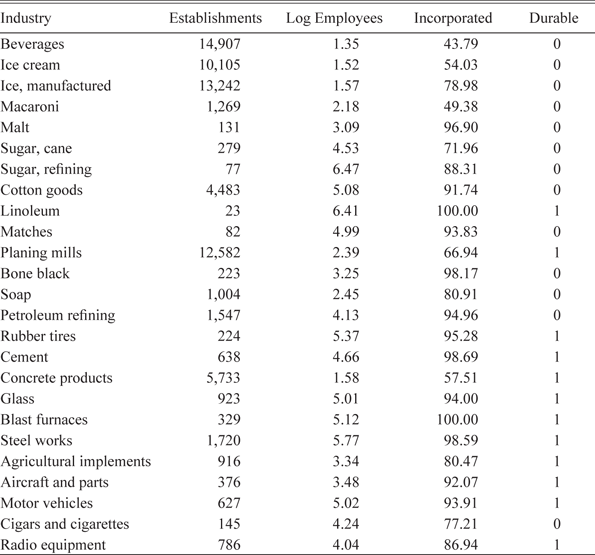
We use the COM, for which the original, establishment-level schedules from 1929, 1931, 1933, and 1935 are available in their original form at the National Archives in Washington, DC.Footnote 5 The COM was collected in other years, including during the Depression, but the establishment-level schedules from the first half of the twentieth century do not exist other than for these four years. The schedules provide a wealth of detail, including a breakdown of outputs and inputs into quantities and values. For our purposes, there is also information on labor use broken down by type of worker, number employed, and total earnings. We draw on a sample of 25 industries summarized in Table 1.Footnote 6 As discussed in the paper by Vickers and Ziebarth (2019), the sample is the work of many different people who collected industries for their own individual purposes.Footnote 7 While not chosen to be representative, these industries cover a wide variety of manufactured products from business durables to consumer non-durables to “high tech” products such as radios, autos, and aircraft. Table 2 shows that our sample comprises about 20 percent of the total value of output in manufacturing, 10 percent of the establishments, and 20 percent of the total wage bill.
SUMMARY STATISTICS FOR THE INDUSTRIES IN OUR SAMPLE

Notes: All statistics are calculated pooling all the census years. The column “Establishments” is the total number of establishments. The column “Log Employees” is the average number of log employees including both white- and blue-collar workers. The column “Incorporated” is the percentage of establishments that are incorporated. We equally weight the establishments in calculating the average size and the percentage. The column “Durable” is whether we coded an industry’s major product as durable.
Sources: Authors’ calculations.
PERCENT OF NATIONAL TOTAL COVERED BY OUR SAMPLE

Notes: All of the national totals are from the 1935 published report on the COM. Besides reporting the values for 1935, it also reported the previous years’ totals.
Sources: Authors’ calculations.
The sample was built in this “curated” way rather than by, for example, randomly sampling some unit such as the establishment for a number of reasons. First, given how the schedules are organized at the National Archives, it is much easier to sample industries than, say, geographic units because the schedules are arranged by industry and then by state within an industry. We also did not sample at the establishment-level since, in our view, this would have limited the value provided by the establishment-level nature of the original schedules. For one, there are a number of important questions about competitive behavior in this period that require complete data from a particular industry. For example, Chicu, Vickers, and Ziebarth (2013) and Vickers and Ziebarth (2014) use the schedules from two industries to study collusion under the National Industrial Recovery Act (NIRA). In addition, one of the benefits of establishment-level data is the ability to follow establishments over time. If we just randomly sampled establishments, for example, this would lead to a very small set of establishments that we observe in multiple years (even ignoring the high rates of turnover). We also did not sample entire industries randomly for the simple fact that we thought certain industries were of more interest than others for the purposes of studying the Depression.
On the balance, we would argue that our sample is fairly representative of manufacturing as a whole. In the Online Appendix, we provide a number of maps showing the geographic coverage of our sample in terms of manufacturing totals at the county level. On county-level demographic and economic characteristics, we show in the Online Appendix that our sample is (slightly) over-representative of counties that grew faster between 1920 and 1930, voted more Democratic in presidential elections, had lower literacy rates, and had more African Americans.Footnote 8 We would argue that these demographic differences reflect the fact that the textile industry, which is part of our sample, dominates southern manufacturing, and so the geographic areas where the coverage of our sample is highest tend to be predominantly from the South. As for economic characteristics, there are only minor differences if we consider bank failure rates or the change in retail sales. Finally, in the Online Appendix, we show that, in 1929, industries that make up our sample are similar to those industries not in our sample in terms of size as measured by employment and revenue, as well as revenue per blue-collar worker and earnings per blue-collar worker.
Similar to the papers by Davis and Haltiwanger (Reference Davis and Haltiwanger1991) and Atack, Bateman, and Margo (ABM) (2004), we will run regressions explaining labor earnings with establishment-level covariates. Davis and Haltiwanger (Reference Davis and Haltiwanger1991), who work with the post-1963 COM, include size as measured by number of employees, age, ownership, energy costs, product specialization, and capital intensity as well as regional and industry fixed effects. ABM (2004), who work with the nineteenth-century COM, include number of employees, capital intensity, use of steam power, as well as regional and industry fixed effects. In the COM data we employ, information about region, industry, and size as measured by total employment (or our preferred measure of revenue) is all available. On the other hand, the information on age is sparse. The form for the 1929 census asks if the plant had begun operation before 1 January 1928, but other than that, there is no information on age. None of the other censuses ask such a question.Footnote 9 We also have information on the incorporation status of an establishment as well as whether the establishment is part of a single-plant or multiplant firm, as used by Davis and Haltiwanger (Reference Davis and Haltiwanger1991).Footnote 10 As for other variables emphasized by Davis and Haltiwanger (Reference Davis and Haltiwanger1991), we have information on energy used for 1929 and 1935 only. The most important limitation of our COM data is the lack of a measure of capital. There are, in some cases, industry-specific measures of physical capital stock; for example, the amount of compression capacity in the manufactured ice industry. However, nothing is systematic enough to use in regressions pooling across industries and years.
Skill Categories and Their Comparability across Years
We now turn to a discussion of how we measure the skill of the workers and their earnings. The forms do not provide any information on, for example, educational attainment of workers. Instead, we will distinguish between wage and salaried employees, or what we will call blue- and white-collar jobs. Blue-collar workers were presumably mainly production workers on the factory floor, but they could also include hourly janitorial staff or workers on the loading dock. White-collar workers in this classification were clerks, administrative officers, and office workers, generally. In the modern COM, the labor force breakdown provided is into production and non-production workers. Dunne, Haltiwanger, and Troske (1997) defend the use of non-production workers as a measure of skilled workers. Our breakdown is quite similar to this.Footnote 11 All of our salaried workers would fall into the modern category of non-production workers. On the other hand, there are surely some hourly workers, such as janitors, that would be classified as non-production workers in the modern taxonomy but are blue-collar wage earners in ours.
For blue-collar workers, in all four censuses, the form asks for the number of wage earners employed in each month.Footnote 12 In computing earnings per blue-collar worker, we divide the total annual wage bill by the average of the monthly employment figures. As noted by Rosenbloom and Sundstrom (1999), the Census Bureau itself cautioned about how to interpret the wage earner employment number. In particular, it listed some possible reasons why the employment numbers are inflated relative to the true number of full-time equivalent employees. First, the establishments might have reported part-time workers as well. Second, workers that were laid off might have stayed on the payroll for a time and still been potentially counted as working at the establishment. The earnings variable is much more straightforward and comes from a question that does not change over the years asking for the “total amount paid to wage earners.”Footnote 13
For the white-collar skill group, the computation of earnings per worker is somewhat more complex. First, we exclude officers and proprietors from the totals since we have no information about their earnings. Next, in 1929, the Census Bureau asked about the number of “managers, superintendents, and other responsible administrative employees; foremen and overseers who devote all or the greater part of their time to supervisory duties; clerks, stenographers, bookkeepers, and other clerical employees on salary,” as well as the total amount that this group was paid. In 1933, this category is split between the managers and clerks, which are reported separately along with their total wage bills, with no mention of foremen.Footnote 14 For 1935, the same three white-collar categories of officers, managers, and clerks are reported, with the total number of clerks being reported for four separate months. Unfortunately, the 1931 census form does not contain any information about the number of or payment to white-collar workers.
Establishment-Level Earnings Measurement
To emphasize, we will be comparing earnings per worker by “collar” color computed by dividing total earnings by total workers in that type of job at an establishment. The establishment-level nature of this measure is different than much of the rest of the literature on inequality that measures worker-level variation in earnings. All earnings are measured in 2015 dollars adjusting for inflation using the consumer price index for urban households (CPI-U). The 1 percent tails are winsorized to limit the role of measurement error. Winsorizing or trimming the tails of the distributions is common in the literature that works with (modern) establishment-level data, e.g., Davis and Haltiwanger Reference Davis and Haltiwanger1991. ABM (2004) also trim the tails in their dataset from the nineteenth-century COM.Footnote 15
To clarify the relationship between the measures at the establishment and worker levels, let y be worker-level earnings and x be an establishment identifier (ignoring the skill dimension for now). Then, the law of total variance states
 $$Var\left( y \right) = Var\left( {E\left[ {y{\rm{|}}x} \right]} \right) + E\left[ {Var\left( {{\rm{|}}x} \right)} \right],$$
where Var(y) is the worker-level variance of earnings,  $Var\left( {E\left[ {y{\rm{|}}x} \right]} \right)$ the variance of average earnings between establishments, and
 $E\left[ {Var\left( {y{\rm{|}}x} \right)} \right]$ the average variance of earnings within an establishment.Footnote 16 What we actually observe is the term $Var\left( {E\left[ {y{\rm{|}}x} \right]} \right)$, the establishment-level variance of earnings per worker. So, our establishment-based measure of inequality will underestimate worker-level inequality because we do not observe the within-establishment term $E\left[ {Var\left( {y{\rm{|}}x} \right)} \right]$, which is strictly positive. Because of this, the levels of our inequality measures are not directly comparable to others in the literature using worker-level data.
The relevant question for us is whether changes in our measure reflect changes in worker-level inequality, which, in turn, depends on the changes in within-establishment inequality. The most plausible theory in our view, based on modern evidence (Solon, Barsky, and Parker 1994) as well as in the Depression where the evidence is much more indirect (Lebergott Reference Lebergott1989; Margo Reference Margo1991; Sundstrom Reference Sundstrom1992), is that the least productive and lowest paid workers within an establishment are the first to be fired, meaning $E\left[ {Var\left( {y{\rm{|}}x} \right)} \right]$ would decline in recessions. This would imply that changes in our measure of inequality $Var\left( {E\left[ {y{\rm{|}}x} \right]} \right)$understate changes in the worker-level measure Var(y).
An additional question in measuring earnings per worker is how to handle establishments that report no employees (and, hence, pay nothing to workers) yet have positive revenue. These make up a non-trivial fraction of establishments in our dataset and presumably are cases where the owner, besides managing the establishment’s operations, also works directly in production. Margo (2015) discusses this same problem in the nineteenth-century COM and its effects on estimates of the returns to scale of the production function. While potentially important for the question of returns to scale and estimating overall labor income shares, it is not obvious what effects these establishments have on earnings inequality of workers, our particular interest. One could construct scenarios where the individuals running these businesses are, on average, more able; therefore, their shadow earnings as an employee are high relative to the mean of the observed earnings distribution. One might also imagine that, because the owner has to perform many different tasks, he is relatively less productive than a worker specialized in doing one task. In this case, the shadow earnings as an employee of a sole proprietor would be low relative to the mean of the observed distribution. While both of these theories would affect the level, it is more difficult to see how they would affect changes in measured inequality. In the end, we have chosen to drop this set of establishments.
CHANGES IN THE EARNINGS DISTRIBUTIONS
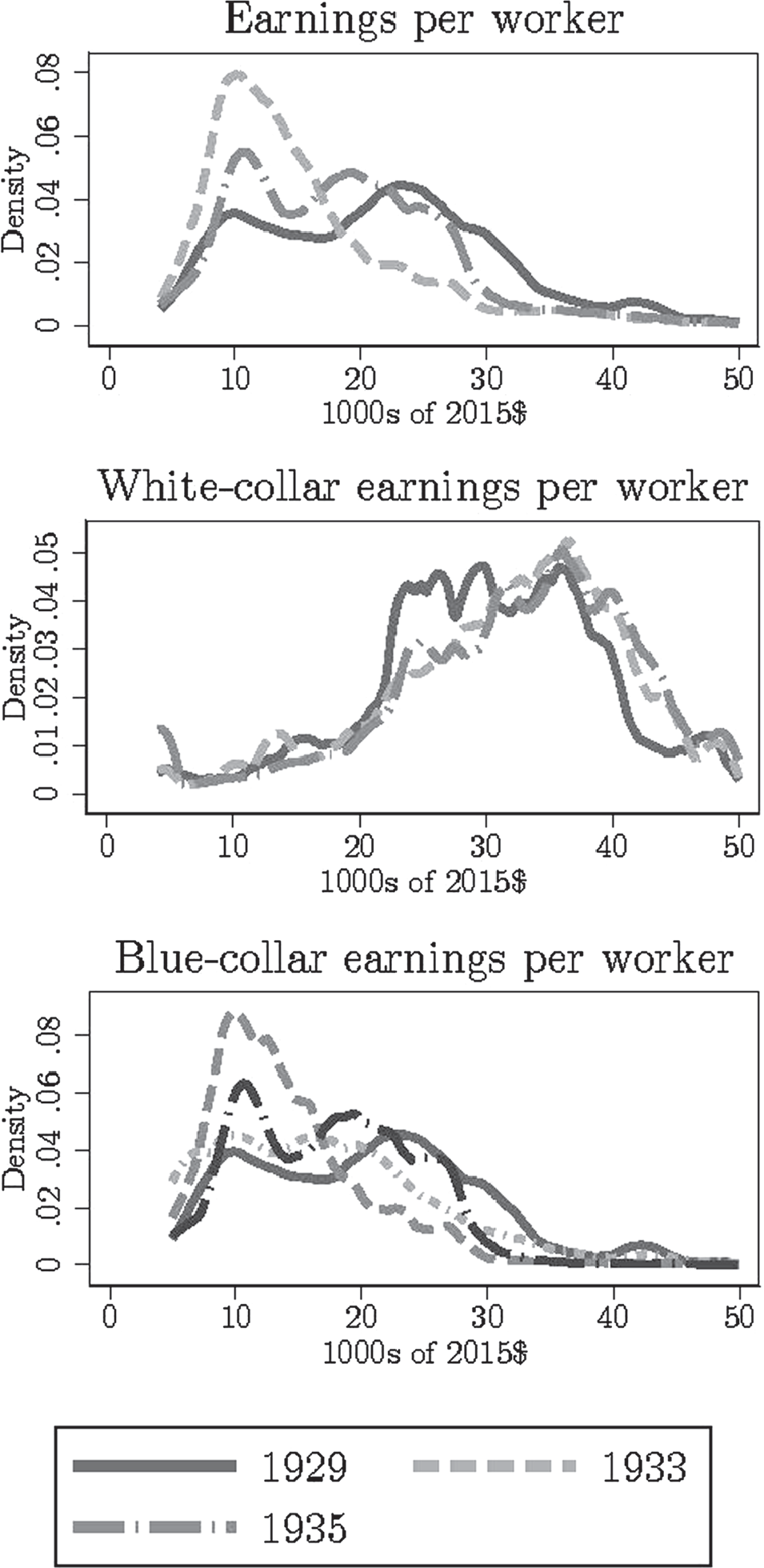
The first panel of Figure 1 shows the overall distribution of earnings pooling blue- and white-collar workers, where each establishment is weighted by the number of workers in that skill group. We emphasize that this distribution is not the true distribution of worker earnings in manufacturing, since we are implicitly treating all workers at a given establishment as earning the same amount. This will surely mask variation in earnings within an establishment and skill group, so the inequality measures based on this distribution will be lower than the measures from the distribution where we observed every individual employee’s earnings. However, the Davis and Haltiwanger (Reference Davis and Haltiwanger1991) decomposition for modern data shows that over half of the variance in manufacturing earnings per hour inequality can be accounted for by between-establishment differences. This suggests that a substantial fraction of changes in the worker-level earnings distribution can be captured using changes in establishment-level earnings distribution.
DISTRIBUTIONS OF EARNINGS PER WORKER

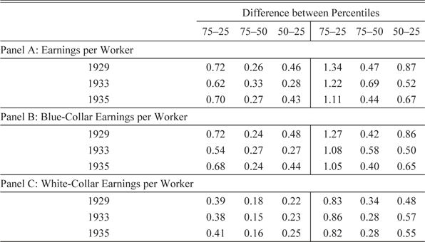
The distribution goes from being bimodal in 1929 to unimodal in 1933 and then back again in 1935. Panel A of Table 3 reports the changes in various differences in percentiles for this distribution. Focusing on the 75–25 measure of inequality, there is a decline in 10 log points between 1929 and 1933. By 1935, the 75–25 differential is nearly back to its pre-Depression 1929 value. We consider this as evidence that the Depression did not have permanent effects on the “bulk” of the manufacturing earnings distribution as reflected in the 75–25 differential. On the other hand, the 90-10 inequality measure shows a decline over this six-year period, though this is almost totally concentrated in the distribution of earnings for blue-collar workers, a point we return to later.
SUMMARY STATISTICS OF EARNINGS VARIABLES

Notes: The statistics correspond to the difference between the two percentiles listed. Each establishment is weighted by the number of workers in the particular color group. All variables are log transformed.
Sources: Authors’ calculations.
These findings need to be qualified since this is the distribution of earnings for those employed and the Depression is a time of large declines in the number of people working.Footnote 17 To think about the effects of changes on this margin, assume that, with probability 1 − p, a person receives 0 income and, with complementary probability, a person receives income w drawn from distribution F with standard deviation σ. We think of this setup as capturing a case where there is a fixed pool of “manufacturing workers” who work in that sector or are unemployed (and receive nothing). Then, the standard deviation of the earnings distribution, including those who are unemployed, is  $SD\left( w \right) = p\sigma $, or, in log differences,
 ${\rm{\Delta }}\log \left( {SD\left( w \right)} \right) = {\rm{\Delta }}\log \left( p \right) + {\rm{\Delta log}}\left( \sigma \right)$. The second term,
 ${\rm{\Delta log}}\left( \sigma \right)$, is what we are estimating here. Note that decreases in p, which are increases in manufacturing unemployment, all else equal, reduce overall inequality. This is because, in our example, all unemployed workers receive earnings of 0. The same logic would apply if those that became unemployed received an income draw from some less dispersed distribution (though the effect on changes in overall inequality would be more muted).
We now decompose the overall earnings into the distributions for blue- and white-collar workers in the other panels of Figure 1. Quite clearly, the qualitative changes in the overall earnings distribution are being inherited from the blue-collar earnings distribution. The 1929 and 1935 distributions for white collar are nearly identical. Panels B and C of Table 3 report the changes in the differences in percentiles for these distributions. As is evident from the figures, the changes in the overall earnings distribution are driven by changes in the blue-collar earnings distribution. This is also due to the fact that blue-collar workers make up the lion’s share of total employment. So, the overall earnings distribution places much more weight on changes in the blue-collar distribution.Footnote 18
DECOMPOSITION OF THE EARNINGS DISTRIBUTION
We now decompose the sources of those changes using the procedure developed by JMP (1993). We write the earnings per worker at establishment i in year t as
 $${y_{it}} = {X_{it}}{\beta _t} + {u_{it}},$$
where yit is log earnings per worker, Xit a vector of observables characteristics, and uit a residual unobserved component. The observable characteristics include establishment-level characteristics as well as whether the earnings correspond to white- or blue-collar workers. The “white-collar” indicator is an estimate of the skill premium in establishment-level earnings per worker. Let F t be the distribution of the residuals, which is potentially time varying.Footnote 19 Then,  ${u_{it}} = F_t^{ - 1}\left( {{\theta _{it}}} \right)$, where θit is the percentile of establishment i in year t in the earnings distribution.
Changes in the earnings distribution can come from three possible sources: (1) changes in average establishment characteristics Xit (“observables” in the language of JMP); (2) changes in the relationship between these characteristics and earnings, represented by βt (“prices”); or (3) changes in the distribution of unobservables Ft (“residuals”). To see this analytically, take 1929 as the base year and define  $\bar \beta = {\hat \beta _{1929}}$ and
 ${\bar F^{ - 1}}\left( {{\theta _{it}}} \right) = \hat F_{1929}^{ - 1}\left( {{\theta _{it}}} \right)$. Now, if the distribution of residuals and the coefficients βt were fixed over time, then earnings would be
 $$y_{it}^1 = {X_{it}}\bar \beta + {\bar F^{ - 1}}\left( {{\theta _{it}}} \right).$$
Changes in the distribution of Yit are those attributable to changes in the observable characteristics of the establishments. Now, if the coefficients β t can change as well as the value of the covariates Xit, then earnings would be
 $$y_{it}^2 = {X_{it}}{\beta _t} + {\bar F^{ - 1}}\left( {{\theta _{it}}} \right).$$
Any additional change in the distribution of  $y_{it}^2$ relative to
 $y_{it}^1$ is due to changes in the returns to observables, what JMP call prices. Finally, if we further allow the distribution of residuals to change, then earnings are given by
 $$y_{it}^3 = {X_{it}}{\beta _t} + F_t^{ - 1}\left( {{\theta _{it}}} \right),$$
which is the actual level of earnings. Any additional changes to  $y_{it}^3 = {y_{it}}$ relative to
 $y_{it}^2$ can be attributable to changes in the residuals.
To understand what we will report in the end, let Yt be a statistic of the earnings distribution in year t such as the interquartile range (d7525) or the 90–10 gap (d9010). Also, let  $Y_t^k$ be the same statistic calculated using the distribution of
 $y_{it}^k$ for k = 1,2,3. Then, we write the following decomposition:
 $${Y_t} - {Y_{1929}} = \left[ {Y_t^1 - Y_{1929}^1} \right] + \left[ {\left( {Y_t^2 - Y_{1929}^2} \right) - \left( {Y_t^1 - Y_{1929}^1} \right)} \right] + \left[ {\left( {Y_t^3 - Y_{1929}^3} \right) - \left( {Y_t^2 - Y_{1929}^2} \right)} \right],$$
where we will refer to the first term on the right-hand side as the “observables” term, the second as the “prices” term, and the third as the “residuals” term, while the term on the left-hand side is what we call the “totals” term. These four terms are what we will report. By construction, each of these terms will be equal to 0 in 1929 and clearly the sum of the three components on the right-hand side will equal the total change in the statistic between year t and 1929.
It is important to remember that this is just an accounting decomposition and should not be interpreted structurally. Besides the original paper by JMP, a number of authors working with manufacturing data have employed this procedure, such as Davis and Haltiwanger (Reference Davis and Haltiwanger1991) using modern COM data and ABM (2004) using the nineteenth-century COM. In estimating the regression and constructing the residuals, we “pool” both blue- and white-collar workers and weight each establishment-“color” group by the number of workers in that group. For the vector of characteristics Xit, we include in the log of revenue a binary variable for whether the establishment is part of an incorporated firm, whether the firm owns multiple establishments or plants, as well controls for Census regions and industry along with the white-collar indicator.Footnote 20
Table 4 shows the results from the regressions for each year pooling both types of workers weighted by the number of employees with robust standard errors.Footnote 21 First, and not surprisingly, we find a large skill premium—more precisely, difference in average earnings between white- and blue-collar workers—of 34 log points in 1929, increasing to 72 points in 1933, and falling back to 55 log points. While Goldin and Margo (1992) report an increase between 1929 and 1933 in the ratio of monthly income for clerks to laborers in the railroad industry of about 21 log points, these numbers are not strictly comparable, as our blue-collar workers are not “unskilled” and white-collar workers include all salaried workers, not clerks only. Qualitatively speaking, the skill premium patterns we identify are consistent with the summary of Goldin and Margo (1992, p. 16): “Although inequality [as measured by the skill premium] widened at the beginning of the 1930s, it narrowed after 1933 […] Most series we have uncovered show little overall change from 1929 to 1939, although the wage structure changed within the decade.”Footnote 22
REGRESSIONS OF EARNINGS PER WORKER

Notes: The earnings per worker variable is log transformed and the 1 percent tails are winsorized. In addition to white-collar status, the set of controls includes log revenue, dummies for incorporation and multiplant status, as well as region and industry fixed effects. An observation is an establishment and each establishment is weighted by the number of employees in a particular color group. The excluded region is New England. Standard errors are robust. *p < 0.1, **p < 0.05, and ***p < 0.01.
Sources: Authors’ calculations.
There is a significant and stable establishment size premium across all three years, with the coefficient on (log) revenue between 0.05 and 0.07.Footnote 23 This positive size premium is consistent with modern literature on this relationship (Davis and Haltiwanger Reference Davis and Haltiwanger1991). On the other hand, this is different from the patterns in the nineteenth century, as estimated by ABM, who broadly speaking find a negative size gradient. They interpret this negative gradient in the context of the Goldin and Katz (1998) model of skill-technology complementarity. A positive relationship is relatively straightforward to explain in a model with differences in productivity, decreasing returns to scale, and rent sharing. Then, higher productivity firms have higher labor demand and, hence, are larger. Furthermore, they share this higher productivity with their workers due to a less than perfectly competitive labor market.
The overall pattern of the regional differences in average earnings (the New England region is the excluded category) is as expected, with a large negative coefficient associated with being located in the South and all regions having lower average earnings than New England. What is striking is the decline between 1929 and 1933 in the penalty for being in the South, which includes the East and West South Central as well as the South Atlantic regions. These findings echo the results of Rosenbloom and Sundstrom (1999), who find that the Depression was comparatively mild in the South after controlling for industry composition (and long-run trends).
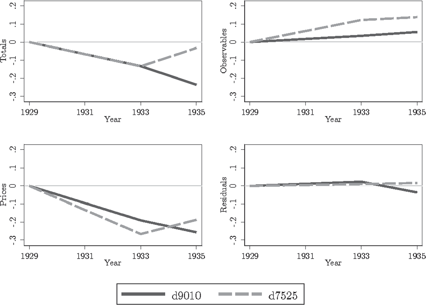
In Figure 2, we show the values from the JMP decomposition for all workers, taking 1929 as the base year and defining changes relative to that year.Footnote 24 We plot the decomposition results for both the difference between the 75th and 25th percentiles (d7525) and the difference between the 90th and 10th percentiles (d9010). The totals figure replicates the pattern observed in the summary statistics of a fanning out of the earnings distribution in 1933 and then a return to the pre-Depression spread by 1935 in the 75–25 differential. Clearly, changes in the residuals play no role, and while changes in observables matter slightly, the vast majority of the changes in inequality, as measured by the 75–25 differential, are driven by changes in prices or the returns to observables. The fact that prices matter is similar to the original paper by JMP, who argue that much of the increase in earnings per week inequality between 1963 and 1989 was due to increases in the returns to skill (though a substantial role is still played by changes in the residuals). On the other hand, ABM find almost no role is played by changes in prices in explaining increasing dispersion in earnings per month during the nineteenth century. Instead, two-thirds of the increase are due to increasing residual dispersion and the rest to changes in observables.Footnote 25
JMP DECOMPOSITION OF EARNINGS PER WORKER

The compression in regional earnings differences is the main reason why changes in the prices component explain much of the changes in inequality. While the convergence of the South with New England is consistent with the findings in Wright (Reference Wright1997, Table 7.7, p. 217), the timing is not consistent with Wright’s explanation. He argues that this convergence was due to the minimum wages imposed by the NIRA, which had a stronger effect in the South because of the region’s relatively lower average wages. However, the NIRA was not passed until June 1933, and furthermore, the minimum wages were set on an industry-by-industry basis in a so-called “Code of Fair Competition.” In addition, many of these codes specified lower minimum wages for establishments operating in the South.
There were other policies beyond the NIRA that may have had regionally heterogeneous effects. During the decline, the responses of the regional Federal Reserve banks to the collapse of the banking industry were quite heterogeneous. The Atlanta Federal Reserve was on one extreme in responding aggressively to limit the fallout from the panics. On the other extreme, the actions of the St. Louis Federal Reserve, at best, abated the panics and, at worst, exacerbated them (Richardson and Troost Reference Richardson and Troost2009). In the recovery period, New Deal spending was allocated in a heterogeneous way across the country with some areas favored for political reasons (Wallis Reference Wallis1998). We leave it to future work to examine the role of these policies on regional convergence.
While changes in regional differences tended to reduce inequality between 1929 and 1933, the increase in the skill premium between 1929 and 1933 worked in the opposite direction. Why might the skill premium change over the business cycle? One reason might be that the elasticity of substitution between high and low skilled labor is not equal to one so that changes in demand lead to changes in relative demand for these two types of labor. Our finding that the skill premium rose is suggestive that, in response to declines in output demand, establishments wanted to substitute away from unskilled labor toward skilled. Another interpretation for the changing skill premium is that there are differing levels of selection on unobserved productivity between these groups. In particular, our results are consistent with establishments first laying off the least productive and lowest paid skilled worker. This would lead to an increase in the average earnings of skilled relative to unskilled. It just so happens in our quantitative results that the changes in the geographic differences dominate the changes in the skill premium and so price changes end up contributing to a decline in inequality.
THE ROLE OF ESTABLISHMENT ENTRY AND EXIT
We now study the role of the extensive margin of establishment entry and exit in driving changes in the earnings distribution in manufacturing. To do this, we exploit the panel structure of our dataset. To get a sense of the importance of the extensive margin for employment, we can decompose the change in total employment between two consecutive censuses ∆Emp into changes due to entry and exit as well as continuing establishments. By definition,
 $${\rm{\Delta }}Em{p_t} = {\rm{\Delta }}Emp_t^{CONT} + Emp_t^{Entered} - Emp_{t - 1}^{Exiting},$$
where  ${\rm{\Delta }}Emp_t^{CONT}$ is change in total employment for continuing establishments between consecutive censuses,
 $Emp_t^{Entered}$ is total employment of newly entered establishments in the current census, and
 $Emp_{t - 1}^{Exiting}$ is total employment of exiting establishments in the preceding census. Between 1929 and 1933, more than 100 percent of the change in blue-collar employment, and 70 percent for white-collar employment, can be explained by exit. This shows the important role played by the extensive margin of establishment entry and exit for total employment.
The fact that the extensive margin played such a large role should not be surprising given the tremendous amount of churn in establishments during this period of time. In particular, in our sample, about 60 percent of the establishments appeared in only a single year. What is perhaps surprising is that this churn is due not just to particularly high rates of exit but also high rates of entry.Footnote 26 Unlike the modern COM, the Census Bureau at this time did not assign unique identifiers to establishments, which would allow for (relatively) error-free linking over time. Instead, our definition of entry and exit is defined as whether we are able to identify a particular establishment over time based on the “sticky” information reported on the schedules. This information includes the name of the establishment and its location. One concern is whether this churn is simply due to measurement error. To the extent that this measurement error is uncorrelated with observable characteristics, it will generate an attenuation bias that obscures differences in earnings between continuing, entered, and exiting establishments.Footnote 27
A number of papers using these data (Chicu, Vickers, and Ziebarth 2013; Ziebarth Reference Ziebarth2015; Hansen and Ziebarth 2017; Vickers and Ziebarth 2019) have examined this issue of linking establishments in a variety of ways, from examining particular industries with external data sources to internal data checks on whether exit is predictable. All of them come to the conclusion that these links reflect real exits and entries. Finally, we note that this rate of churn is not orders of magnitude greater than the rate in the modern COM. For example, Dunne, Roberts, and Samuelson (1989) find five-year exit rates for manufacturing establishments of around 36 percent in the “normal” period of the 1970s.Footnote 28
The relationship between establishment entry and exit and the earnings distribution depends, in part, on whether what drives entry and exit is correlated with earnings. One closely studied driver of establishment survival in this period is productivity. While the literature disagrees about the proper way to measure productivity, whether in terms of physical output or revenue, there is wide agreement that it is an important determinant of exit.Footnote 29 Furthermore, in regressions not reported here, we document a positive relationship between productivity and earnings in the data. So, at least the establishment-level connection between the extensive margin and earnings is a plausible one.Footnote 30
We study skill group earnings across establishments comparing those establishments that enter or exit relative to those that continue. In particular, for skill group s at establishment i observed in COM t,Footnote 31 we estimate cross-sectional regressions for (log) earnings per worker Yit that include dummies for entry and exit:
 $${y_{ist}} = {\beta _1} \cdot Exitin{g_{it}} + {\beta _2} \cdot Entere{d_{it}} + {X_{ist}}\gamma + {\varepsilon_{it}}.$$
Regressions are weighted using employment weights and Xist includes the same set of controls as the JMP regressions. There are a few issues of timing worth noting. First, the exit indicator is defined as whether the establishment exits between COM t and the next COM t + 1. This means that the exit indicator in 1929 is based on whether an establishment exited by 1931, not 1933 when we next have information on blue-collar earnings. On the other hand, the entry indicator is defined as whether the establishment enters between COM t − 1 and COM t. Thus, the entry indicator in 1933 is based on whether the establishment entered between 1931 and 1933, not 1929 and 1933.Footnote 32 Because of this timing convention, we can only include both entry and exit indicators in 1933. For 1929, we do not know the entry status of an establishment, and for 1935, we do not know the exit status.
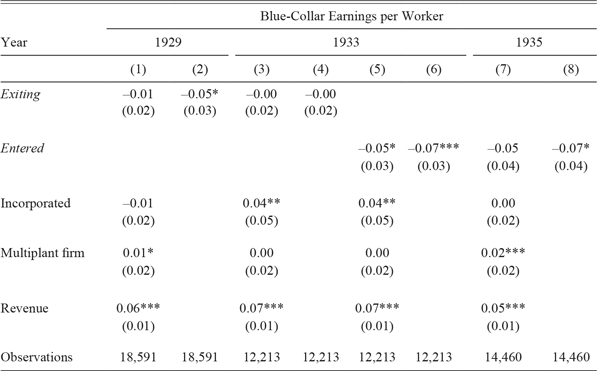
Table 5 reports the results of these regressions for exit and entry for blue-collar workers by year. To make the regressions easier to compare within a year, we hold fixed the set of establishments included, those within a year that are not missing any of the covariates. On the one hand, Columns (1)–(4) of Table 5 show that, in general, exiting establishments pay less than continuing establishments, though this is sensitive to controlling for other observables. The 5 log point penalty in 1929 after controlling for industry and region almost completely disappears with the additional controls, particularly log revenue. On the other hand, Columns (5)–(8) show a very stable penalty associated with entry of between 5 and 7 log points across specifications and years.
THE EXTENSIVE MARGIN AND BLUE-COLLAR EARNINGS PER WORKER

Notes: The earnings per worker variable is log transformed and the 1 percent tails are winsorized. All regressions include region and industry fixed effects. Standard errors are robust and the regression is weighted by employment totals. The variable Exiting is a binary for whether an establishment will exit between the current and next census. The variable Entered is a binary for whether an establishment entered between the current and preceding census. Because of this timing convention, we only observe exit status in 1929 and 1933 and entry status in 1933 and 1935. *p < 0.1, **p < 0.05, and ***p < 0.01.
Sources: Authors’ calculations.
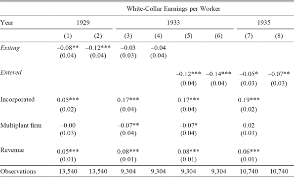
Table 6 reports the same set of regressions for white-collar workers. We find in Columns (1)–(4) that, unlike blue-collar workers, there is a negative relationship between earnings per worker and exit. This penalty of around 3–4 log points is smaller in magnitude in 1933 than in 1929 when it is 8–12 log points. Columns (5)–(8) show that, consistently, across years and specifications, establishments that enter pay less than continuing establishments. These penalties range from 5 log points in the case of 1935 with additional controls to 14 log points in 1933 with no controls. Taken together, these results, which show, on the whole, that earnings per worker are related to the entry and exit of establishments, provide motivating evidence for the role of the extensive margin in contributing to changes in the earnings distribution.
THE EXTENSIVE MARGIN AND WHITE-COLLAR EARNINGS PER WORKER

Notes: The earnings per worker variable is log transformed and the 1 percent tails are winsorized. All regressions include region and industry fixed effects. Standard errors are robust and the regression is weighted by employment totals. The variable Exiting is a binary for whether an establishment will exit between the current and next census. The variable Entered is a binary for whether an establishment entered between the current and preceding census. Because of this timing convention, we only observe exit status in 1929 and 1933 and entry status in 1933 and 1935. *p < 0.1, **p < 0.05, and ***p < 0.01.
Sources: Authors’ calculations.
Quantifying the Effects of the Exit Margin
We now study how changes in exit affect the observed earnings distribution by considering a counterfactual that imputes earnings and employment for exiting establishments. To do this, we first estimate the following specification on the set of surviving establishments between adjacent censuses:
 $${\rm{\Delta }}{y_{it + 1}} = \beta {X_{it}} + {\varepsilon_{it}},$$
where Xit includes log revenue and fixed effects for year, state, and industry.Footnote 33 With these regression results (not reported here), we impute earnings per worker for exiting establishments based on their characteristics as  ${\hat y_{it + 1}} = {y_{it}} + \hat \beta {X_{it}}$. The assumption is that exits are random once we condition on the pre-determined observables Xit. Under this assumption, we can predict the earnings of exiting establishments based on the growth rate of earnings for continuing establishments with similar characteristics. Put differently, we assume that, after conditioning on a set of observables, there are no unobservables that simultaneously determine whether an establishment exits and its employment or earnings growth. This assumption does not imply that the levels of earnings for exiting and continuing establishments are necessarily the same conditional on observables. Instead, our assumption is consistent with an establishment having to pay too high of wages as an explanation for its subsequent exit. Our assumption does require that, in the counterfactual of this establishment not exiting, it would still continue to pay relatively high wages in the next census.
We also assume that there are no general equilibrium effects. That is, the distribution of earnings at continuing establishments would be unaffected in the counterfactual of no exits. To impute counterfactual employment for weighting the distribution, we use the same approach as when imputing earnings. Note that the “actual” distributions in 1933 and 1935 exclude any establishments entering in those years, respectively. This is why the actual distributions here will differ from the actual distributions in the entry counterfactual that we discuss later. So, these figures show how the distribution of earnings would have evolved for establishments in the preceding census if there had been no exit.
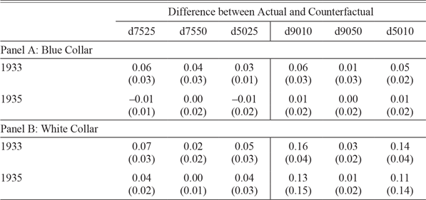
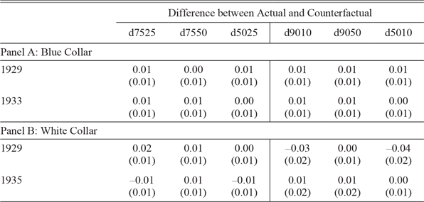
Table 7 shows the difference between the counterfactual and actual measure of inequality over time for the two skill groups.Footnote 34 We calculate standard errors for these statistics using a bootstrap procedure that samples with replacement within the strata of year and industry. We then calculate these statistics using the bootstrap sample and repeat this 50 times. We report the standard deviation of the bootstrap values of each statistic. For the blue-collar distribution in 1933, both the 75–25 and 90–10 differentials would have been 6 log points higher, about one-third of the change (see Panel B of Table 3), if there had been no exit. Based on the bootstrap errors and an assumption of asymptotic normality, this is a statistically significant change. Exit between 1933 and 1935 appears to have no statistically or economically significant effect on inequality. For the white-collar distribution, exit plays a substantial role in compressing inequality. For example, the 90–10 differential would have been 16 log points higher in 1933 if not for exit and 13 points in 1935, though this change is not statistically significant. Given the small changes in the white-collar inequality measures overall (see Table 3), the counterfactual analysis shows that exit masked a large change in inequality for white-collar workers in continuing establishments. In both of these years, the differences are driven mainly by the lower tail of the earnings distribution. Exiting establishments pay white-collar workers less than do continuing establishments, conditional on observables, so removal of these relatively low earning paying firms plays a compressive role. Taken together, these results support the “first out” theory, where the lowest paying establishments, which are perhaps the lowest productivity, are the first to exit in a downturn. These exits lead to a decline in the establishment-level earnings distribution mainly driven by compression in the difference between the median and lowest percentiles. However, this mechanism is not symmetric in that we do not observe the exit margin pushing up inequality during the recovery period of 1933–1935. One possible explanation is that, during periods of rising demand, exits tend to be driven more by “idiosyncratic” shocks.
ROLE OF ESTABLISHMENT EXIT ON THE EARNINGS PER WORKER DISTRIBUTION

Notes: Standard errors are in parentheses and are based on 50 bootstrap replications. Each establishment is weighted by the number of workers in the particular color group. All variables are log transformed. The statistic “d7525” is the difference between the 75th and 25th percentiles, “d7550” the difference between the 75th and 50th percentiles, “d5025” the difference between the 50th and 25th percentiles, “d9010” the difference between the 90th and 10th percentiles, “d9050” the difference between the 90th and 50th percentiles, and “d5010” the difference between the 50th and 10th percentiles.
Sources: Authors’ calculations.
Quantifying the Effects of the Entry Margin
Our next counterfactual considers the extensive margin of entry. The counterfactual we compute removes the earnings differential associated with entrants based on the results in Columns (6) and (8) of Tables 5 and 6. We then recalculate various measures of inequality for the counterfactual distribution of earnings per worker with entrants’ earnings adjusted in this way.Footnote 35 No adjustment is made to incumbent establishments. We calculate standard errors for these statistics using the same bootstrap procedure described above.
Table 8 shows the difference in some measures of inequality between the counterfactual and the actual distribution.Footnote 36 There are only minor differences due to entry for either blue- or white-collar workers in either year. Relative to some of the statistics related to the exit margin, these entry effects are precisely estimated. We conclude that the entry margin does not work like the “opposite” of the exit margin and plays little role in explaining changes in the earnings distribution.
ROLE OF ESTABLISHMENT ENTRY ON THE EARNINGS PER WORKER DISTRIBUTION

Notes: Standard errors are in parentheses and are based on 50 bootstrap replications. Each establishment is weighted by the number of workers in the particular color group. All variables are log transformed. The statistic “d7525” is the difference between the 75th and 25th percentiles, “d7550” the difference between the 75th and 50th percentiles, “d5025” the difference between the 50th and 25th percentiles, “d9010” the difference between the 90th and 10th percentiles, “d9050” the difference between the 90th and 50th percentiles, and “d5010” difference between the 50th and 10th percentiles.
Sources: Authors’ calculations.
CONCLUSION
We introduce a new, detailed, and comprehensive establishment-level dataset covering a sizable fraction of manufacturing during the Great Depression. These data allow us to study distributional changes in earnings per worker between 1929 and 1935 along a number of dimensions: skill, industry, and geography. Using these data, we find that the 75–25 differential of the overall earnings distribution declined between 1929 and 1933 and then recovered by 1935. From an accounting perspective, this was driven by changes in the blue-collar earnings distribution. The distribution of earnings for white-collar workers was little changed. When decomposing these results, we find that changes in the returns to observable characteristics, particularly skill and geography, explain the bulk of the changes in the earnings distribution.
We then examine the role of the extensive margin of establishment entry and exit in explaining these changes. Using a procedure to impute earnings of exiting establishments, we find that this played an important role in reducing inequality between 1929 and 1933 for blue- and white-collar workers, mainly by reducing the gap between the median and bottom percentiles of the earnings distribution. Conversely, exit played a minor role in the increase in inequality between 1933 and 1935. The entry margin was not important for measured earnings inequality in either year or for either type of skill group. Taken together, these results are consistent with a selection mechanism that operates only on the exit margin only in bad times.
Going forward, it would be interesting to extend beyond the mainly descriptive analysis in this paper to identify drivers of these changes. One potential such driver is New Deal relief spending and relief employment. A number of other papers have examined the effects of New Deal relief spending on employment or total labor earnings.Footnote 37 But there is no work that examines the distributional consequence of this spending. This is an interesting question given that Darby (Reference Darby1978) argues that relief jobs provided by the New Deal were better paid than comparable private sector jobs. We leave it for future work to identify how this spending affected not just average earnings or employment but also the distribution of earnings.
There were also a number of other labor market interventions during this period that would presumably have direct distributional consequences. Taylor (Reference Taylor2011) studies one such policy: work sharing under the President’s Reemployment Agreement of 1933. Using industry-level data from the NBER Macrohistory database, he finds that employment in terms of bodies increased under this program, but there was not much effect on aggregate hours worked. Unsurprisingly, these changes are reflected in declines in pay per worker. A larger labor market policy was the NIRA and its myriad of labor provisions, including the minimum wage and maximum workweek. If one took the view that its effects were mainly through its impacts on the workweek and were largely orthogonal to the earnings distribution, then this policy prevented regional convergence in earnings per worker from happening more quickly than it would have otherwise by artificially suppressing the length of the workweek in the lower wage South. These effects have to be set against the possible effects the NIRA had on reducing regional disparities in hourly wages themselves through minimum wages. We leave disentangling these possible effects of policy-induced changes in inequality for future work.