2. Preliminaries

For an absolutely continuous random variable $Z$, we denote the probability density function (pdf) by $f_Z(\cdot )$, the cumulative distribution function (cdf) by $F_Z(\cdot )$, the reliability/survival function (sf) by $\bar F_Z(\cdot )$, the hazard/failure rate function by $r_Z(\cdot )$, and the reverse hazard/failure rate function by $\tilde {r}_Z(\cdot )$; here $\bar F_Z(\cdot )\equiv 1-F_Z(\cdot )$, $r_Z(\cdot )=f_Z(\cdot )/\bar F_Z(\cdot )$, and $\tilde r_Z(\cdot )=f_Z(\cdot )/F_Z(\cdot )$.

Copula is a very useful notion in describing the dependency structure between components of a random vector. It builds a bridge between a multivariate distribution function and its corresponding one-dimensional marginal distribution functions. The joint cdf of a random vector $\boldsymbol {X}=(X_1,X_2, \ldots,X_n)$ can be written, in terms of a copula, as

\begin{align*} {F}_{\boldsymbol{X}}(x_1,x_2,\ldots, x_n)& =P(X_1\leq x_1,X_2\leq x_2,\ldots,X_n\leq x_n )\\ & =C( F_{X_1}(x_1), F_{X_2}(x_2),\ldots, F_{X_n}(x_n)), \end{align*}

where $C(\cdot )$ is a copula. Similarly, the joint reliability function of $\boldsymbol {X}$ can be represented as

\begin{align*} \bar{F}_{\boldsymbol{X}}(x_1,x_2,\ldots, x_n)& =P(X_1> x_1,X_2> x_2,\ldots,X_n> x_n ) \\ & =\bar C(\bar F_{X_1}(x_1),\bar F_{X_2}(x_2),\ldots,\bar F_{X_n}(x_n)), \end{align*}

where $\bar C(\cdot )$ is a survival copula. In the literature, different types of survival copulas have been introduced to describe different dependency structures between components of a random vector. The commonly used copulas are the Farlie–Gumbel–Morgenstern (FGM) copula, the extreme-value copulas, the family of Archimedean copulas, the Clayton–Oakes (CO) copula, etc. Among all these copulas, the family of Archimedean copulas is the one that has paid more attention from the researchers due to its wide range of capturing the dependency structures. Moreover, these are mathematically tractable, and there is a large number of results available in the literature which can be used on a ready-made basis in different problems. More information on this topic could be found in the monograph written by Nelsen [Reference Nelsen42]. In what follows, we give the definition of the Archimedean copula (see [Reference McNeil and Nĕslehová33]).

Definition 2.1 Let $\phi : [0, +\infty ]\longrightarrow [0,1]$ be a decreasing continuous function such that $\phi (0)=1$ and $\phi (+\infty )=0$, and let $\psi \equiv \phi ^{-1}$ be the pseudo-inverse of $\phi$. Then,

(2.1)\begin{equation} C(u_1,u_2,\ldots,u_n)=\phi\left(\psi(u_1)+\psi(u_2)+\cdots +\psi(u_n)\right),\quad \text{for }(u_1,u_2,\ldots,u_n)\in [0,1]^{n}, \end{equation}

is called the Archimedean copula with generator $\phi$ if $(-1)^{k}\phi ^{(k)}(x)\geq 0$, for $k=0,1,\ldots,n-2$, and $(-1)^{n-2}\phi ^{(n-2)}(x)$ is decreasing and convex in $x\geq 0$.

Stochastic orders are frequently used to compare two random variables/vectors. In the last seven decades, it has widely been used in various disciplines of science and engineering including actuarial science, econometrics, finance, risk management, and reliability theory. In the literature, different types of stochastic orders (namely, usual stochastic order, hazard rate order, dispersive order, Lorenz order, etc.) have been developed to study different kinds of problems. This topic is explicitly covered in the book written by Shaked and Shanthikumar [Reference Shaked and Shanthikumar49]. Below we give the definitions of stochastic orders that are used in this paper (see [Reference Razaei, Gholizadeh and Izadkhah44,Reference Sengupta and Deshpande47,Reference Shaked and Shanthikumar49]).

Like stochastic orders, the notion of stochastic agings is another important concept in reliability theory. Stochastic agings largely describe how a system behaves as time progresses. There are three types of agings, namely, positive aging, negative aging, and no aging. A system has the positive aging property if its residual lifetime decreases in some stochastic sense as time progresses. On the other hand, negative aging describes the scenario where the residual lifetime of a system increases in some stochastic sense as the system ages. No aging means that the system does not age over time. A variety of positive and negative aging classes (namely, IFR, IFRA, DFR, DLR, etc.) have been introduced in the literature to describe different aging characteristics of a system (see [Reference Barlow and Proschan5,Reference Lai and Xie29], and the references therein). For the sake of completeness, we give the following definitions of aging classes that are used in this paper.

Throughout the paper, we use the words “increasing” and “decreasing” to mean “nondecreasing” and “nonincreasing”, respectively. Furthermore, the words “positive” and “negative” mean “nonnegative” and “nonpositive”, respectively. By $a\stackrel {\text {def.}}=b$, we mean that $a$ is defined as $b$. For a twice differentiable function $u(\cdot )$, we write $u'(t)$ and $u''(t)$ to mean the first and the second derivatives of $u(t)$ with respect to $t$. We use the acronyms “i.i.d.” and “d.i.d.” to mean “independent and identically distributed” and “dependent and identically distributed”, respectively. All random variables considered in this paper are assumed to be absolutely continuous with nonnegative supports.

3. Main results

In this section, we first discuss some stochastic comparisons results for series, parallel, and general $r$-out-of-$n$ systems. Then, we study whether a system of used components performs better than a used system with respect to different stochastic orders. Lastly, the closure properties of different aging classes under formations of different systems have been studied.

Let $\tau ^{\phi _1}_{r|n}(\boldsymbol {X})$ and $\tau ^{\phi _2}_{r|n}(\boldsymbol {Y})$ be the lifetimes of two $r$-out-of-$n$ systems formed by two different sets of $n$ d.i.d. components with the lifetime vectors $\boldsymbol {X}=(X_1,X_2,\ldots,X_n)$ and $\boldsymbol {Y}=(Y_1,Y_2,\ldots,Y_n)$, respectively, where the distributions of $\boldsymbol {X}$ and $\boldsymbol {Y}$ are described by the Archimedean copulas with generators $\phi _1(\cdot )$ and $\phi _2(\cdot )$, respectively. Furthermore, let $X_i\stackrel {d}=X$ and $Y_i\stackrel {d}=Y$, $i=1,2,\ldots,n$, for some nonnegative random variables $X$ and $Y$; here $\stackrel {d}=$ stands for equality in distribution. In what follows, we introduce some notation:

\begin{align*} H_i(u)=\frac{u\phi_i'(u)}{1-\phi_i(u)},\quad R_i(u)=\frac{u\phi_i'(u)}{\phi_i(u)},\quad \text{and} \quad G_i(u)=\frac{u\phi_i''(u)}{\phi_i'(u)},\quad u>0, \ i=1,2. \end{align*}

Since $\phi _i(\cdot )$, $i=1,2$, are decreasing convex functions, it follows that $H_i(\cdot )$, $R_i(\cdot )$, and $G_i(\cdot )$ are all negative-valued functions. Furthermore, we write $\tau ^{\phi _1}_{r|n}=\tau ^{\phi _2}_{r|n}=\tau ^{\phi }_{r|n}$ (say), $H_1(\cdot )=H_2(\cdot )=H(\cdot )$ (say), $R_1(\cdot )=R_2(\cdot )=R(\cdot )$ (say), and $G_1(\cdot )=G_2(\cdot )=G(\cdot )$ (say) whenever the distributions of both $\boldsymbol {X}$ and $\boldsymbol {Y}$ are described by the same Archimedean copula with generator $\phi _1(\cdot )=\phi _2(\cdot )=\phi (\cdot )$ (say). Furthermore, we introduce a few more notations as follows:

\begin{align*} & C(u)=\left(\frac{u\phi''(u)}{\phi'(u)}+\frac{u\phi'(u)}{1-\phi(u)}+1\right)=\frac{uH'(u)}{H(u)},\quad u>0,\\ & C_{r,n}^{j}=\left({-}1\right)^{j-r}\binom{j-1}{r-1}\binom{n}{j},\quad 1\leq r\leq j\leq n,\\ & P_{r,n}^{j}(u)=\frac{C_{r,n}^{j}\phi\left(ju\right)}{\sum_{j=r}^{n} C_{r,n}^{j}\phi\left(ju\right)},\quad Q_{r,n}^{j}(u)=\frac{C_{r,n}^{j}\left(1-\phi\left(ju\right)\right)}{1-\sum_{j=r}^{n} C_{r,n}^{j}\phi\left(ju\right)},\quad u>0,\;1\leq r\leq j\leq n,\\ & K_j(u)=\frac{R\left(ju\right)}{R(u)},\quad L_j(u)=\frac{H\left(ju\right)}{H(u)},\quad u>0,\ 1\leq j\leq n. \end{align*}

4. Examples

In this section, we give some examples to illustrate the sufficient conditions used in the previous section. Here, we specifically consider the copulas that are frequently used in practice, namely, the Clayton copula $C(\boldsymbol {u}) =(\prod _{i=1}^{n} u_i^{-\theta } - n + 1)^{-1/\theta }$ with the generator $\phi (t) = (\theta t + 1)^{-1/\theta }$, for $\theta \geq 0$, the Ali-Mikhail-Haq (AMH) copula $C(\boldsymbol {u}) =((1 - \theta )\prod _{i=1}^{n} u_i)/(\prod _{i=1}^{n}(1- \theta +\theta u_i) -\theta \prod _{i=1}^{n} u_i)$ with the generator $\phi (t) = (1 - \theta )/(e^{t}-\theta )$, for $\theta \in [0, 1)$, etc.

We begin with the following example that demonstrates the conditions given in Theorem 3.1(b) and (c), and Theorem 3.6.

Example 4.1 Consider the Archimedean copula with generator

$$\phi(u)=\frac{1-\alpha_{1}}{e^{u}-\alpha_{1}},\quad \alpha_{1} \in[{-}1,1), \ u>0.$$

Then,

$$k_1(u)\stackrel{\text{def.}}=\sum_{j=2}^{3}P_{2,3}^{j}(u)K_j(u)= \frac{(e^{u}-\alpha_{1})\left(\frac{6e^{u}}{(e^{2u}-\alpha_{1})^{2}}-\frac{6e^{2u}}{\left(e^{3u}-\alpha_{1}\right)^{2}}\right)}{\left(\frac{3}{e^{2u}-\alpha_{1}}-\frac{2}{e^{3u}-\alpha_{1}}\right)},\quad u>0,$$

and

$$k_2(u)\stackrel{\text{def.}}=\sum_{j=2}^{3}Q_{2,3}^{j}(u)L_j(u) =\frac{(e^{u}-\alpha_{1})(e^{u}-1)\left(\frac{6e^{u}}{(e^{2u}-\alpha_{1})^{2}}- \frac{6e^{2u}}{(e^{3u}-\alpha_{1})^{2}}\right)}{1-(1-\alpha_1) \left(\frac{3}{e^{2u}-\alpha_{1}}-\frac{2}{e^{3u}-\alpha_{1}}\right)},\quad u>0.$$

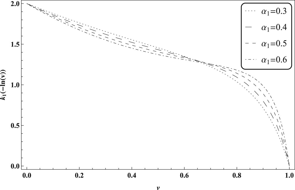
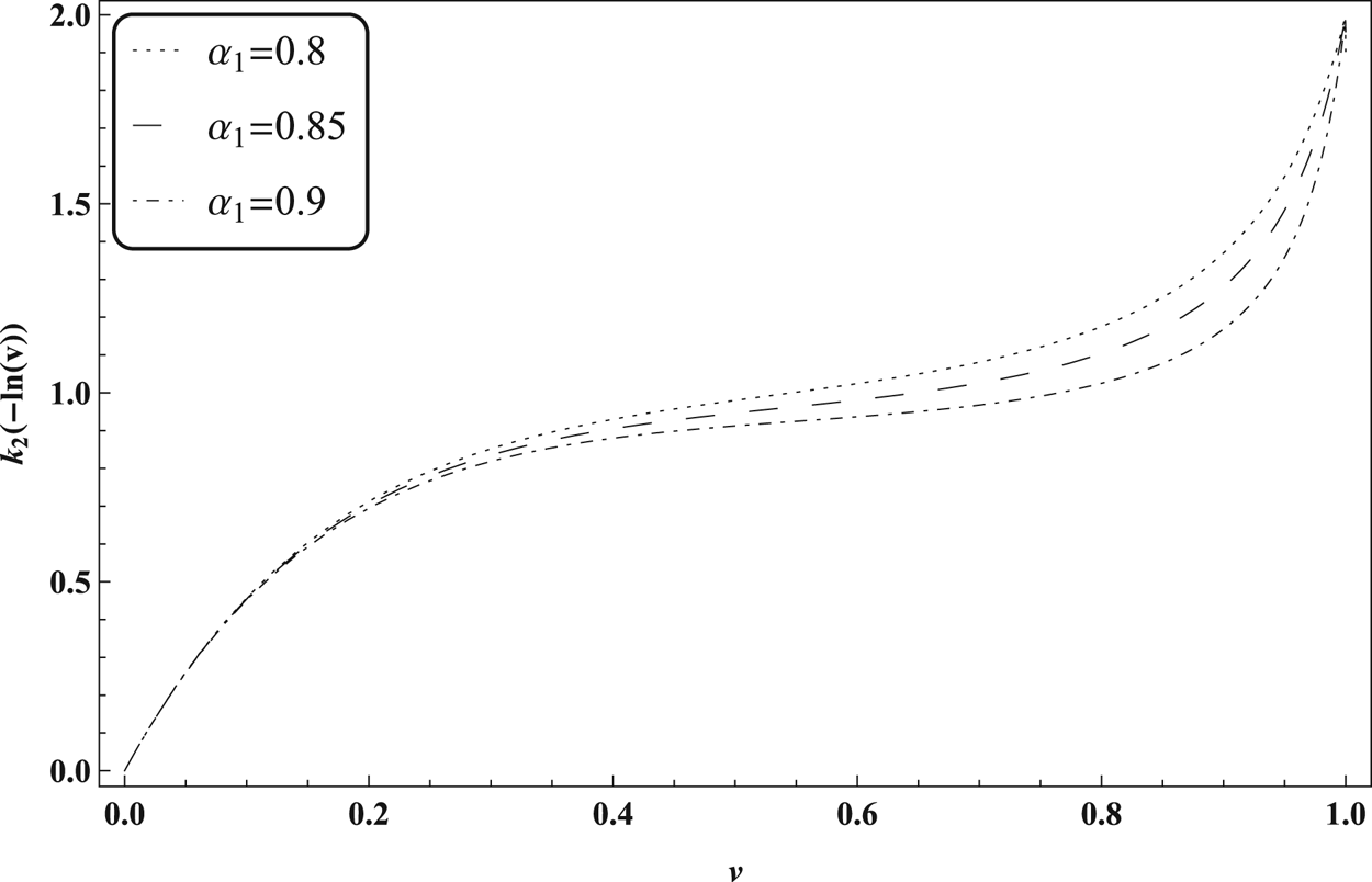
In Figure 1, we plot $k_{1}(-\ln (v))$ against $v\in (0,1]$, for fixed $\alpha _{1}=0.3$, $0.4$, $0.5$, and $0.6$. This shows that $k_{1}(-\ln (v))$ is decreasing in $v\in (0,1]$ and hence, $k_{1}(u)$ is increasing in $u>0$. Furthermore, we plot $k_{2}(-\ln (v))$ against $v\in (0,1]$, for fixed $\alpha _{1}=0.8$, $0.85$, and $0.9$. From Figure 2, we see that $k_{2}(-\ln (v))$ is increasing in $v\in (0,1]$ and hence, $k_{2}(u)$ is decreasing in $u>0$. Thus, the required conditions are satisfied.

Figure 1.

Plot of $k_{1}(-\ln (v))$ against $v\in (0,1]$.

Figure 2.

Plot of $k_{2}(-\ln (v))$ against $v\in (0,1]$.

The following example demonstrates the condition given in Corollary 3.1(c) and (d), Theorem 3.5(c) and (d), Corollary 3.2(a) and (d), and Theorem 3.7(b).

Example 4.2 Consider the Archimedean copula with generator

$$\phi(u)=e^{1-(1+u)^{{1}/{\beta_1}}},\quad \beta_{1} \in(0,\infty), \ u>0.$$

From this, we have

$$R(u)={-}\frac{1}{\beta_1}u(1+u)^{{1}/{\beta_1}-1},\quad \text{for all } u>0,$$

and

$$l_1(u)\stackrel{\text{def.}}=\frac{uR'(u)}{R(u)}=1+\left(\frac{1}{\beta_1}-1\right)\frac{u}{u+1},\quad \text{for all }u>0.$$

It can be easily shown that $l_{1}(u)$ is positive and increasing in $u>0$, for all $\beta _1 \in (0, 1)$. Thus, the required condition holds.

The next example illustrates the condition given in Theorems 3.2(a), 3.5(f), and 3.7(a).

Example 4.3 Consider the Archimedean copula with generator

$$\phi(u)=e^{({1}/{\gamma_1})(1-e^{u})}, \quad \gamma_1 \in(0,1],\ u>0.$$

Then

$$l_2(u)\stackrel{\text{def.}}=\frac{uG'(u)}{G(u)}=\frac{\gamma_1-e^{u}-ue^{u}}{\gamma_1-e^{u}}\quad \text{and} \quad l_3(u)\stackrel{\text{def.}}=\frac{G(u)}{R(u)}=1-\frac{\gamma_1}{e^{u}}, \quad u>0.$$

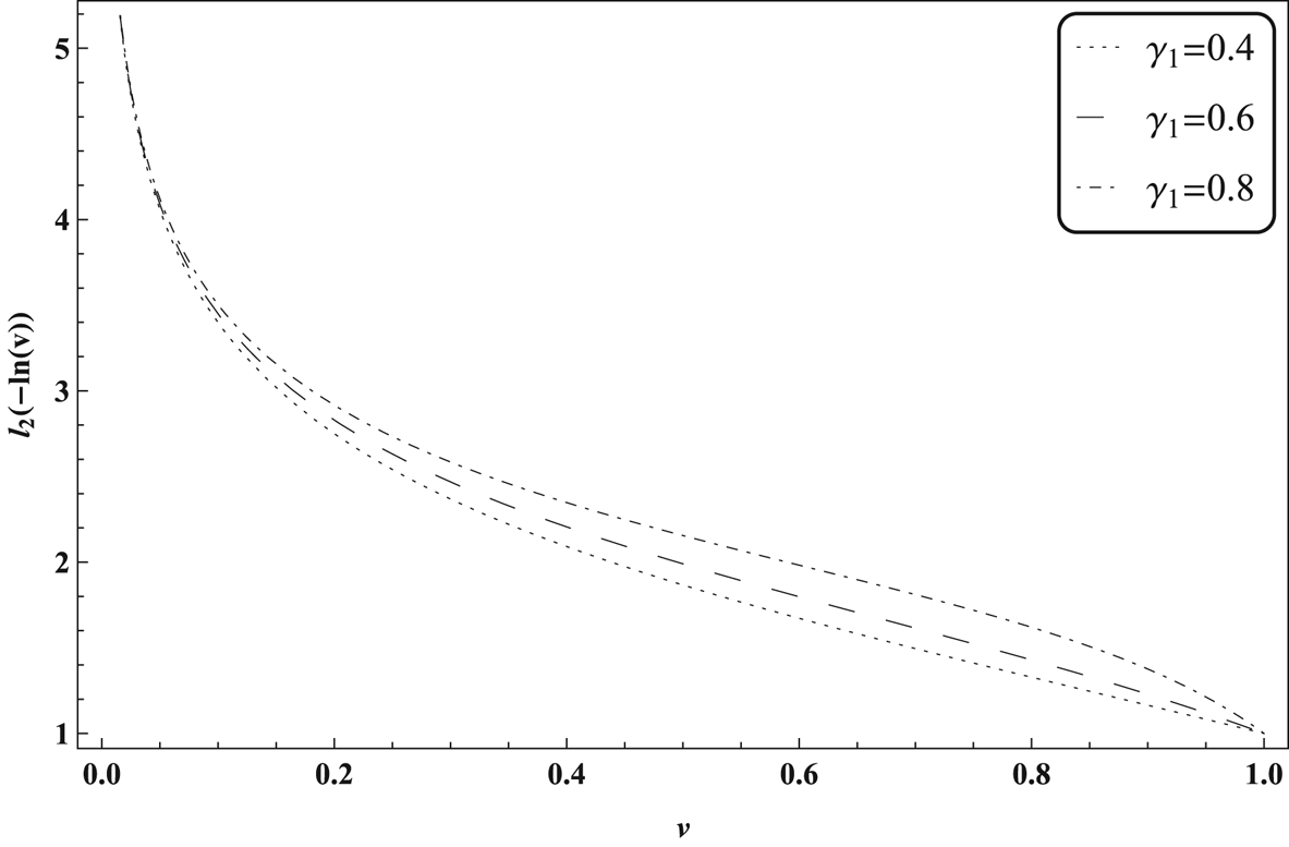
Let us fix $\gamma _1=0.4$, $0.6$, and $0.8.$ In Figure 3, we plot $l_2(-\ln (v))$ against $v\in (0,1]$. This shows that $l_2(-\ln (v))$ is positive and decreasing in $v\in (0,1]$ and hence, $l_2(u)$ is positive and increasing in $u>0$. Furthermore, it can easily be checked that $l_3(u)$ is increasing in $u>0$. Thus, the required condition holds from Remark 3.1.

Figure 3.

Plot of $l_2(-\ln (v))$ against $v\in (0,1]$.

Below we cite an example that illustrates the condition given in Theorem 3.2(b) and (c), and Theorem 3.5(g).

Example 4.4 Consider the Archimedean copula with generator

$$\phi(u)=e^{{-}u^{{1}/{\alpha_2}}},\quad \alpha_2 \in[1,\infty), \; u>0,$$

which gives

$$R(u)={-}\frac{1}{\alpha_2}u^{{1}/{\alpha_2}}\quad \text{and}\quad C(u)=\frac{1}{\alpha_2}-\frac{u^{{1}/{\alpha_2}}e^{{-}u^{{1}/{\alpha_2}}}}{\alpha_2\left(1-e^{{-}u^{{1}/{\alpha_2}}}\right)}-\frac{1}{\alpha_2}u^{{1}/{\alpha_2}},\quad u>0.$$

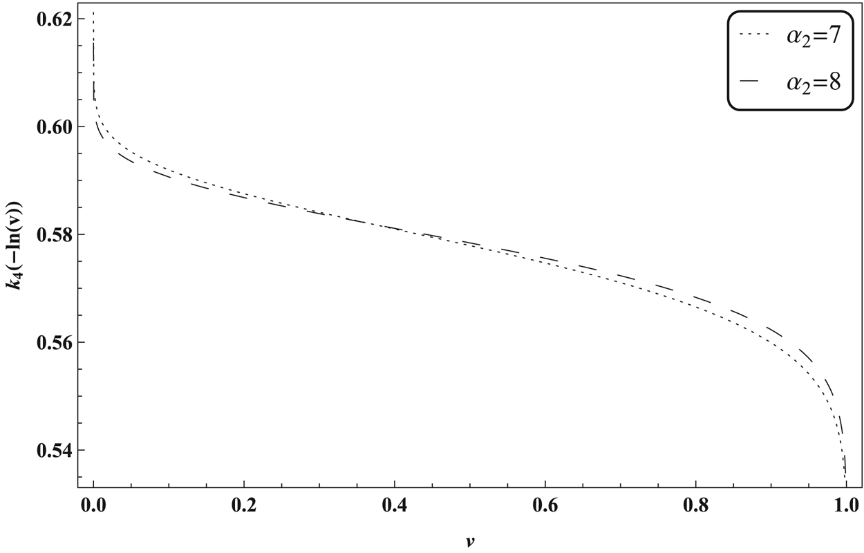
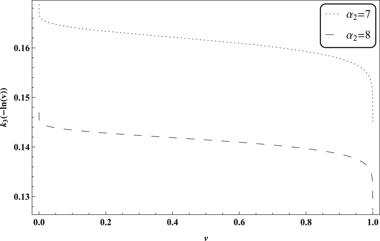
Let us fix $\alpha _2=7$ and $8$. Furthermore, let $k_{3}(u)=uC'(u)/C(u)$ and $k_{4}(u)=C(u)/R(u),$ for $u>0$. From Figures 4 and 5, we see that both $k_{3}(-\ln (v))$ and $k_{4}(-\ln (v))$ are decreasing and positive for all $v\in (0,1]$. Hence, both $k_{3}(u)$ and $k_{4}(u)$ are increasing and positive for all $u>0$. Thus, the required conditions hold from Remark 3.1.

Figure 4.

Plot of $k_{3}(-\ln (v))$ against $v\in (0,1]$.

Figure 5.

Plot of $k_{4}(-\ln (v))$ against $v\in (0,1]$.

The next example demonstrates the condition given in Theorem 3.3(b). Furthermore, this may also be used to illustrate the condition given in Corollary 3.1(b) and (e), Theorem 3.5(b) and (e), and Corollary 3.2(b) and (c).

Example 4.5 Consider two parallel systems $\tau ^{\phi _1}_{1|n}(\boldsymbol {X})$ and $\tau ^{\phi _2}_{1|n}(\boldsymbol {Y})$, where $X\le _{\textrm {hr}}Y$. Consider the Archimedean copulas with generators

$$\phi_1(u)=1-(1-e^{{-}u})^{{1}/{\beta_2}},\quad\beta_2 \in[1,\infty),\ t>0,$$

and

$$\phi_2(u)=\frac{1-\gamma_2}{e^{t}-\gamma_2},\quad\gamma_2 \in[{-}1,1),\ t>0,$$

respectively. Consequently,

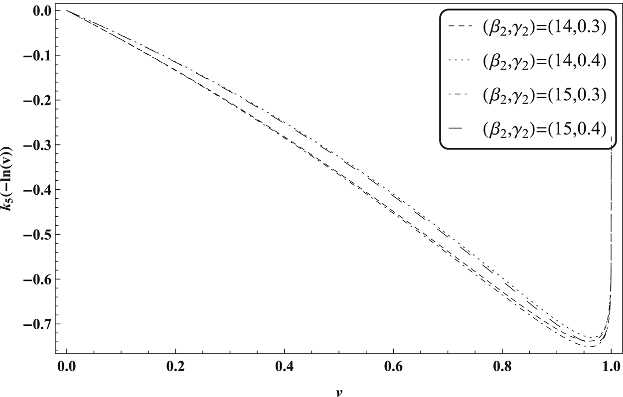
$$k_5(u)\stackrel{\text{def.}}=\phi_1(u)-\phi_2(u)=(1-(1-e^{{-}u})^{{1}/{\beta_2}})-\left(\frac{1-\gamma_2}{e^{u}-\gamma_2}\right), \quad u>0.$$

Let us fix $(\beta _2,\gamma _2)=(14, 0.3),(14,0.4),(15,0.3)$, and $(15,0.4)$. Figure 6 shows that $k_5\left (-\ln \left (v\right )\right )$ is negative for all $v\in (0,1]$ and hence, $k_5(u)$ is negative for all $u>0$. Thus, $\phi _1(u)\leq \phi _2(u)$, for all $u>0$, which, by Remark 3.2, gives $\psi _1(w) \leq \psi _2(v)$, for all $0\leq v\leq w\leq 1$. Again,

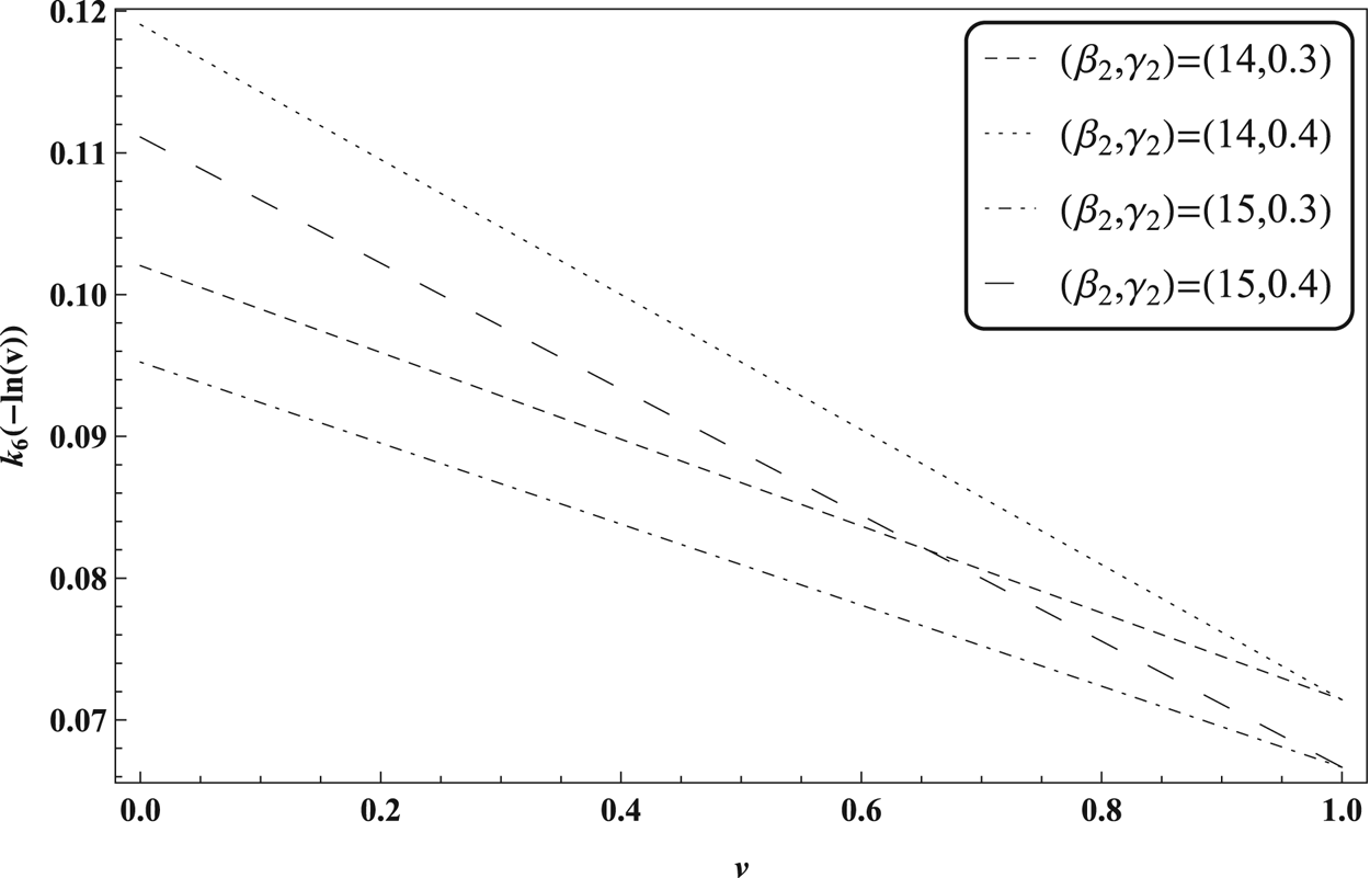
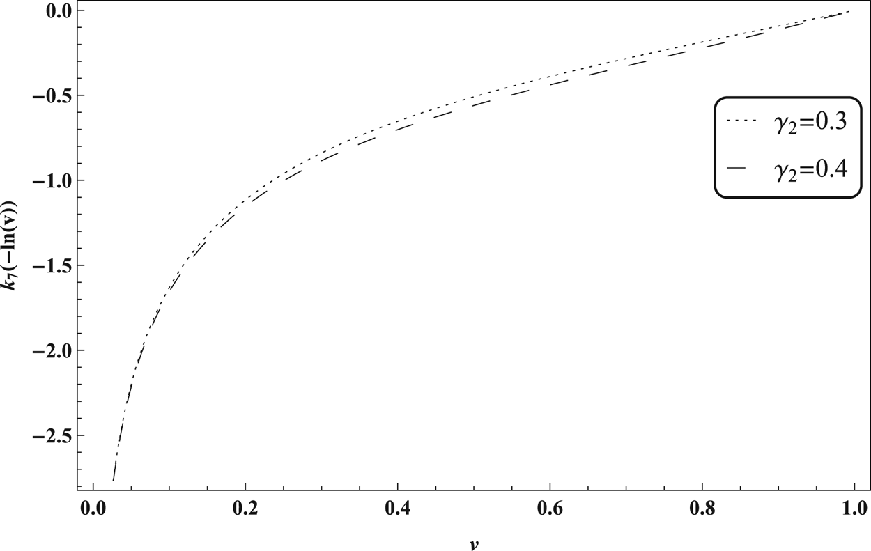
\begin{align*} & k_6(u)\stackrel{\text{def.}}=\frac{H_1(u)}{H_2(u)}=\frac{e^{u}-\gamma_2}{\beta_2\left(1-\gamma_2\right)e^{u}}\\ \text{and}\quad & k_7(u)\stackrel{\text{def.}}=\frac{uH_2'(u)}{H_2(u)}={-}\frac{ue^{u}}{e^{u}-\gamma_2}-\frac{ue^{u}}{e^{u}-1}+1+u,\quad u>0. \end{align*}

From Figure 7, we see that $k_6(-\ln (v))$ is decreasing in $v\in (0,1]$, whereas Figure 8 shows that $k_7(-\ln (v))$ is increasing and negative for all $v\in (0,1]$. Hence, $k_6(u)$ is increasing in $u>0$, and $k_7(u)$ is decreasing and negative for all $u>0$. Thus, the condition of Theorem 3.3(b) holds.

Figure 6.

Plot of $k_5\left (-\ln \left (v\right )\right )$ against $v \in \left (0,1\right ].$

Figure 7.

Plot of $k_6(-\ln (v))$ against $v \in \left (0,1\right ]$.

Figure 8.

Plot of $k_7(-\ln (v))$ against $v \in \left (0,1\right ]$.

Below we give an example that illustrates the condition given in Theorem 3.4(a).

Example 4.6 Consider the Archimedean copulas with generators

$$\phi_1(u)={-}\frac{1}{\alpha_3}\ln(e^{{-}u}(e^{-\alpha_3}-1)),\quad\alpha_3 \in(-\infty,\infty)\setminus \{0\},\ u>0,$$

and

$$\phi_2(u)=(1+\beta_3 u)^{-{1}/{\beta_3}},\quad \beta_3 \in[0,\infty),\ u>0,$$

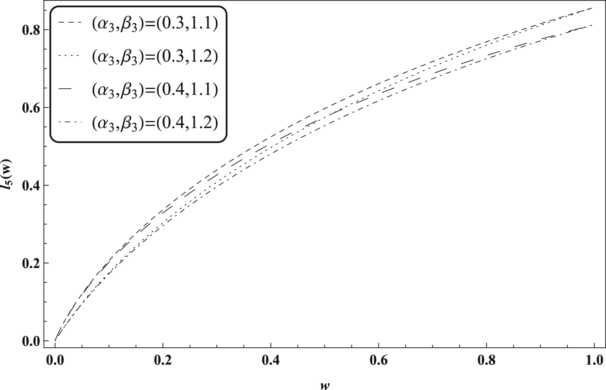
respectively. By writing $l_{5}(w)=\phi _1^{-1}(w)/\phi _2^{-1}(w)$, we have

$$l_{5}(w)=\beta_3\frac{\ln(e^{-\alpha_3}-1)-\ln(e^{-\beta_3 w}+1)}{(w^{-\beta_3}-1)},\quad w\in(0,1].$$

In Figure 9, we plot $l_5(w)$ against $w\in (0,1]$, for fixed $(\alpha _3,\beta _3)=(0.3, 1.1),(0.3, 1.2),(0.4, 1.1)$, and $(0.4, 1.2)$. This shows that $l_5(w)$ is increasing in $w\in (0,1]$, and hence, the condition of Theorem 3.4(a) is satisfied.

Figure 9.

Plot of $l_{5}(w)$ against $w\in (0,1]$.

The following example demonstrates the conditions given in Theorem 3.4(b).

Example 4.7 Consider the Archimedean copulas with generators

$$\phi_1(u)=\frac{1}{1+u^{{1}/{\alpha_4}}},\quad\alpha_4 \in[1,\infty),\ u>0,$$

and

$$\phi_2(u)=e^{{-}u^{{1}/{\beta_4}}},\quad\beta_4 \in[1,\infty), \ u>0,$$

respectively. Consequently,

$$l_{6}(u)\stackrel{\text{def.}}=\phi_1(u)-\phi_2(u)=\frac{1}{1+u^{{1}/{\alpha_4}}}-e^{{-}u^{{1}/{\beta_4}}},\quad u>0.$$

Let us fix $(\alpha _4,\beta _4)=(3.8, 13),(3.8,16),(4.9,13)$, and $(4.9,16)$. In Figure 10, we plot $l_{6}\left (-\ln \left (v\right )\right )$ against $v\in (0,1]$. This shows that $l_{6}\left (-\ln \left (v\right )\right )$ is positive for all $v\in (0,1]$ and hence, $l_{6}(t)$ is positive for all $u>0$. Thus, $\phi _1(u)\geq \phi _2(u)$, for all $u>0$, which, by Remark 3.2, gives $\psi _1(w)\geq \psi _2(v)$, for all $0\leq w\leq v\leq 1$. Again,

$$l_{7}(u)\stackrel{\text{def.}}=\frac{R_1(u)}{R_2(u)}=\frac{\beta_4t^{{1}/{\alpha_4}}}{\alpha_4(1+u^{{1}/{\alpha_4}})u^{{1}/{\beta_4}}} \quad \text{and}\quad \frac{uR_2'(u)}{R_2(u)}=\frac{1}{\beta_4}, \quad u>0.$$

In Figure 11, we plot $l_{7}(-\ln (v))$ against $v\in (0,1]$. This shows that $l_{7}(-\ln (v))$ is decreasing in $v\in (0,1]$ and hence, $l_{7}(u)$ is increasing in $u>0$. Furthermore, it is trivially true that ${uR_2'(u)}/{R_2(u)}$ is increasing in $u>0$. Thus, the required conditions are satisfied.

Figure 10.

Plot of $l_{6}\left (-\ln \left (v\right )\right )$ against $v\in \left (0,1\right ]$.

Figure 11.

Plot of $l_{7}(-\ln (v))$ against $v\in \left (0,1\right ]$.

The following example demonstrates the condition given in Theorem 3.7(c).

Example 4.8 Consider the Archimedean copula with generator

$$\phi(u)=\frac{\gamma_3}{\ln(u+e^{\gamma_3})},\quad \gamma_{3} \in(0,\infty),\ u>0,$$

which gives

$$H(u)={-}\frac{\gamma_3u}{(u+e^{\gamma_3})(\ln(u+e^{\gamma_3})-\gamma_3)\ln(u+e^{\gamma_3})},\quad \text{for all } u>0.$$

Let us fix $\gamma _{3}=3$, $4$, and $5$. By writing $l_{8}(u)=H(u)/(\ln \left (1-\phi (u)\right )),$ $u>0$, we plot $l_{8}(-\ln (v))$ against $v\in (0,1]$. From Figure 12, we see that $l_{8}(-\ln (v))$ is decreasing in $v\in (0,1]$ and hence, $l_{8}(u)$ is increasing in $u>0$. Thus, the required condition is satisfied.

Figure 12.

Plot of $l_{8}(-\ln (v))$ against $v\in (0,1]$.

5. Concluding remarks

In this paper, we consider different coherent systems (especially, series, parallel, and general $r$-out-of-$n$ systems) formed by d.i.d. components, where the dependency structures are described by Archimedean copulas. We provide some sufficient conditions (in terms of the generators of Archimedean copulas) to show that one system performs better than another one with respect to the usual stochastic order, the hazard rate order, the reversed hazard rate order, the likelihood ratio order, and the aging faster orders in terms of the failure rate and the reversed failure rate. In the same spirit, we compare a used system and a system made by used components with respect to different stochastic orders. Furthermore, we study the closure properties of different aeing classes (namely, IFR, DFR, DRFR, ILR, DLR, IFRA and DFRA) under the formation of $r$-out-of-$n$ systems. Moreover, we illustrate the proposed results through various examples.

As we discussed, the main idea of this paper is to consider the dependency structure between components of a system by an Archimedean copula. Most of the systems used in real life have inter-dependency structures between their components, and hence, the assumption of “independent components” sometimes oversimplifies the actual scenario. Thus, we consider the coherent systems that are formed by dependent components governed by the Archimedean copula. As mentioned in the Introduction section, Archimedean copulas are extensively used in the literature due to their wide spectrum of capturing the dependency structures. Furthermore, Archimedean copulas enjoy nice mathematical properties which make them popular. Thus, our study based on the Archimedean copulas may be useful in different practical scenarios where systems with dependent components are considered.

Even though we derived a large number of results in this paper, there remains ample scope to develop further results for systems with dependent components under the Archimedean copula. Here, we only consider the systems with dependent and identically distributed components. The same study for the systems with dependent and nonidentically distributed components may be considered in future.