What is already known?

• • Meta-analysis is central to empirical science.

• • Advanced methods are often out of reach for researchers and students with limited programming skills.

What is new?

• • We implemented a comprehensive set of standard and advanced meta-analytic methods through the Meta-Analysis module in JASP, an open-source statistical software program.

Potential impact for RSM readers

• • The JASP graphical user interface enables users across technical backgrounds to run state-of-the-art meta-analyses with only a couple of mouse actions.

• • This manuscript provides an overview of the meta-analysis tools available in the Meta-Analysis module.

3.1. Effect size computation

We begin by loading the csv dataset (available from https://osf.io/mb56t/) into JASP via the “ $\equiv $ ” button in the top left corner of the application and the “Open” option. Once the dataset is loaded into JASP, we proceed by computing effect size estimates and their standard errors from the case counts. This is done in the “Effect Size Computation” menu underneath the “Meta-Analysis” module heading (Figure 1). In the left input panel, the “Design,” “Measurement,” and “Effect size” dropdowns determine which effect size is computed, and the variable inputs (e.g., “Group 1/Outcome +” and “Group 1/Outcome -”) map dataset columns to the calculations. The right output panel then shows how many effect sizes were computed successfully. Notice that the output panel dynamically updates as the options are selected; “run” or “execute” commands are usually not needed in JASP.

Figure 1.

Effect size computation menu in JASP.

Figure 1. Long description

The interface is divided into two main vertical panels.

Left Panel: Effect Size Computation Menu.

- Top Section: Design is set to Independent groups, Measurement to Binary, and Effect size to R R.

- Variable Selection: A list of variables including trial, author, year, tpos, tneg, cpos, and cneg is on the left. Arrows point to assigned fields on the right. Group 1/Outcome + (Events) is assigned to tpos. Group 1/Outcome - (Non-Events) is assigned to tneg. Group 2/Outcome + (Events) is assigned to cpos. Group 2/Outcome - (Non-Events) is assigned to cneg.

- Frequency/event cell adjustment: Add 0.5 to Only zero is selected. Drop studies with no cases/events is set to No.

- Options: Show metafor R code is checked. Computed Columns Names are defined as computed effect size, computed standard error, and computed effect size type.

Right Panel: Results Preview.

- Title: Bacillus Calmette-Guerin (B C G) Vaccines.

- Summary Table: Shows Step 1, Effect Size R R, Computed 13, Total Computed 13. A note states effect sizes were successfully computed and added to the dataset.

- Metafor R Code: Displays the R script using the escalc function with arguments including ai = tpos, bi = tneg, ci = cpos, di = cneg, add = 0.5, to = ‘only0’, measure = ‘R R’, and data = dataset.

Behind the scenes, “Effect Size Computation” calls the metafor::escalc function. As such, the analysis supports a wide range of effect sizes suitable for many different settings. The corresponding R code can be generated using the “Show metafor R code” option in the “Options” section. Furthermore, the analysis allows for the chaining of multiple calculations with the green “+” button and can restrict computations to subsets of rows via the corresponding “Subset” variable input. Details about the available effect sizes and the required variable input are available through the “(i)” help button in the top-right of the input section.

3.2. Funnel plot

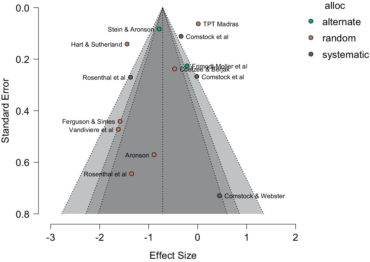
Next, the data are visualized with a funnel plot. Funnel plots are a useful tool for visual inspection of the data before proceeding with the analyses; for instance, funnel plots can help identify odd patterns, incorrectly extracted information (e.g., standard errors mistaken for standard deviations), and are used to examine the data for “small-study effects.”

The funnel plot is created using the “Funnel Plot” menu. The analysis requires specification of the computed “Effect Size” and “Effect Size Standard Error” variable inputs. By default, JASP shows a scatterplot of the effect sizes against their standard errors with a funnel that reflects the sampling distribution centered at the random-effects estimate (Figure 2; a second funnel under the null hypothesis can be created via the “ $\mathcal {H}_0$ ” checkbox). In the “Estimates Mapping” subsection, the “Study Label” option is set to the “author” variable and the “Color” option is set to the “allocation” variable, which extends the funnel plot with the author labels and allocation color coding. The figure can be exported in various file formats via the small triangle just above the plot.

Figure 2.

Funnel plot created in JASP.

Figure 2. Long description

The X axis represents Effect Size ranging from negative 3 to 2. The Y axis represents Standard Error on an inverted scale from 0.0 at the top to 0.8 at the bottom. A central vertical dotted line is positioned at an effect size of approximately negative 0.7. A large triangular shaded region, or funnel, originates from the top center and widens toward the bottom. This funnel is divided into three nested layers of increasing transparency, representing different confidence intervals.

Data points are scattered within and around the funnel, labeled with study names. A legend in the top right titled ‘alloc’ identifies three categories:

* alternate (teal circles): includes Stein & Aronson near the apex and Frimodt-Moller et al on the right slope.

* random (orange circles): includes T P T Madras at the top right, Hart & Sutherland on the left, and several others like Ferguson & Simes, Vandiviere et al, Aronson, and Rosenthal et al distributed down the left side.

* systematic (dark grey circles): includes Comstock et al near the top, Coetzee & Berjak, another Comstock et al entry, and Comstock & Webster at the bottom right.

Most studies with lower standard error are clustered near the top apex, while studies with higher standard error spread wider at the base.

Additional options include incorporating heterogeneity into the sampling distribution, displaying power enhancement (“power bands”),Reference Kossmeier, Tran and Voracek ²³ and creating separate funnels for subsets of data. Related statistical tests are in the “Publication Bias/Sensitivity Analyses” section, including funnel plot asymmetry tests,Reference Egger, Smith, Schneider and Minder ^{24 ,} Reference Begg and Mazumdar ²⁵ trim-and-fill,Reference Duval and Tweedie ²⁶ and fail-safe N variants.Reference Rosenthal ^{27 –} Reference Rosenberg ²⁹

3.3. Meta-analysis

We proceed by estimating a random-effects model via the “Meta-Analysis” menu in the “Classical” part of the “Meta-Analysis.” The user interface contains several sections separating it into easy-to-navigate option groups. In the pre-opened data input section, we specify the required “Effect Size” and “Effect Size Standard Error” variable inputs. Default settings follow metafor recommendations, including the “REML” random-effects estimator and the “Knapp and Hartung” adjustment for the fixed-effects test.Reference Knapp and Hartung ³⁰

With the variable input set as in the left panel of Figure 3, the “Meta-Analytic Tests” and “Meta-Analytic Estimates” tables appear in the “Model Summary” output section (right output panel of Figure 3). In this example, the tests reject the null hypothesis that the pooled effect is zero and the null hypothesis of no between-study heterogeneity. Estimates are by default reported on the input scale (i.e., the log risk ratio). To present pooled estimates and confidence/prediction intervals on the risk ratio scale instead, we set the “Exponential” option in the “Transform effect size” dropdown located in the “Statistics” section. This transformation propagates to all effect size estimates in the forest plot, bubble plots, and EMMs.

Figure 3.

Random-effects meta-analysis with forest plot.

Figure 3. Long description

The interface is divided into two main sections.

On the left is a configuration sidebar titled Meta-Analysis and Forest Plot. It contains drag-and-drop variable selection fields for trial, author, year, and effect size. Below this are collapsible menus for Model, Statistics, and Estimated Marginal Means and Contrasts. A Forest Plot settings section at the bottom shows selected variables including label, ablat, cpos, cneg, tpos, and tneg.

On the right is the results output pane.

1. Model Summary: Contains a Meta-Analytic Tests table showing Heterogeneity Q sub (12) = 152.23, p < .001 and Pooled effect t sub (12) = minus 3.95, p = .002. A Meta-Analytic Estimates table lists the Pooled effect estimate as 0.489 with a 95% C I of 0.330 to 0.726.

2. Forest Plot: A graphical representation of 13 studies including Aronson (1948) and Comstock et al (1976). Data columns list Latitude, Contr (+), Contr (-), Treat (+), and Treat (-). The plot shows individual study effect sizes as black squares with horizontal error bars. A vertical dashed line represents the null effect at 1. At the bottom, two diamonds represent the Fixed effect estimate and the Pooled effect on a logarithmic Risk Ratio scale ranging from 0.033 to 3.

3. Metafor R Code: A code block at the bottom shows the underlying script using the rma function with method = ‘REML’ and test = ‘knha’.

Options within the “Statistics” section allow users to obtain additional information about the fitted model, such as relative heterogeneity measures I² and H², fit measures (e.g., log likelihood, AIC, and BIC), and confidence and prediction intervals of different levels. In addition, the “Diagnostics” section presents comprehensive model diagnostics, including casewise diagnostics,Reference Viechtbauer and Cheung ^{31 ,} Reference Viechtbauer, Schmid, Stijnen and White ³² a profile likelihood plot,Reference Raue, Kreutz and Maiwald ³³ the Baujat plot,Reference Baujat, Mahe, Pignon and Hill ³⁴ and the residual funnel plot. Finally, the “Advanced” section contains additional settings that allow advanced users to fully control the metafor::rma.uni function by changing the optimization settings, fixing between-study heterogeneity, extending the R function call directly, and applying permutation tests.Reference Follmann and Proschan ^{35 ,} Reference Good ³⁶ Importantly, the “Advanced” section also allows the R code that corresponds to the fitted model to be generated via the “Generate metafor R code” option. The resulting output, shown at the bottom of Figure 3, can be especially helpful when teaching users of various levels or when attempting a graceful transition to R.

3.4. Forest plot

Forest plots are the most commonly used visualization in meta-analyses and can be created in the “Forest Plot” section. The forest plot can include three components that are toggled independently: “Study information,” “Estimated Marginal Means,” and “Model Information.” To produce the forest plot shown in Figure 3, we select the “Study information” component and specify “Selected Variables” to define study information to be shown on the left side of the study information panel (including information about column titles, centering, etc.). We also select the “Model Information” panel and specify the desired information to be included in the panel (e.g., heterogeneity estimates, fixed-effect estimate, etc.). Final styling, such as modifying the relative width of the left, middle, and right sides of the figure (automatic width adjustment is not always perfect), setting the x-axis label, or the addition of vertical line(s), is controlled in the “Settings” subsection.

Other notable options in the “Study Information” panel include the ability to show predicted effects based on the estimated model, and the ability to aggregate effect size estimates according to a grouping variable, which is especially useful when individual studies contribute multiple effect sizes. The “Settings” subsection controls the details of the output, such as the number of decimals, whether hypothesis tests and/or estimates are reported on the right or left side of the figure, mapping variables to the effect size estimates' color and shape, and additional behavior when a subgroup analysis is specified.

3.5. Subgroup analysis

The first example is completed by performing a subgroup analysis based on the type of treatment allocation. The subgroup analysis is specified via the “Subgroup” variable input. Assigning the allocation variable into the variable input stratifies all previous outputs (tests, estimates, and forest plot) based on the treatment allocation. Furthermore, a new row called “Subgroup differences” is added to the “Meta-Analytic Tests” table with results of a null hypothesis of no differences in the pooled effect across the subgroups. Here, we cannot reject the null hypothesis of no difference between the subgroups ( $p = 0.361$ , not shown).

In the case of binary or person-time outcomes, the Mantel–HaenszelReference Mantel and Haenszel ³⁷ and PetoReference Yusuf, Peto, Lewis, Collins and Sleight ³⁸ methods with equivalent input and output options are available under the “Mantel–Haenszel/Peto” menu of the Meta-Analysis module.

4.1. Meta-regression

Meta-regression examines how study-level predictors (moderators, such as the length of the intervention) relate to the effect size while adjusting for other predictors (e.g., whether participants received feedback). In contrast to subgroup analysis, common between-study heterogeneity is estimated from the full dataset after covariate adjustment (unless, as showcased later, a location-scale model is applied).

After setting the required “Effect Size” and “Effect Size Standard Error” variables in the “Meta-Analysis” menu, the meta-regression specification is completed by assigning the intervention “length” and “feedback” variables to the “Predictors” variable input. Continuous and categorical moderators are handled differently by the analysis, and therefore it is important to verify the variable icons: three intersecting circles indicate a categorical variable, whereas the ruler icon indicates a continuous variable. The complete input for our example is shown on the left side of Figure 4.

Figure 4.

Meta-regression with estimated marginal means and bubble plot.

Figure 4. Long description

The image is a screenshot of a statistical software interface divided into two main sections.

Left Section: Classical Meta-Analysis Control Panel.

* Top area: Variable selection list including id, author, year, grade, and minutes.

* Middle area: Input fields for Effect Size (y i), Standard Error (s e i), Method (Restricted M L), and Predictors (feedback and length).

* Bottom area: Estimated Marginal Means and Contrasts settings with length and feedback selected.

Right Section: Statistical Output.

* Meta-Regression Summary: A table for Terms Tests shows feedback with F equals 0.024 and length with F equals 3.499. A Coefficients table lists estimates for Intercept (0.073), feedback (0.016), and length (0.015).

* Estimated Marginal Means and Contrasts Summary: A table for feedback levels ‘no’ and ‘yes’ shows estimates of 0.216 and 0.232 respectively.

* Bubble Plot: A scatter plot at the bottom right. The Y-axis represents Effect Size from negative 0.5 to 1.5. The X-axis represents length from 0 to 25. Data points are represented by circles of varying sizes, with a solid black regression line and a light gray shaded confidence interval band showing a slight positive linear trend.

The corresponding output shows a “Meta-Regression Summary” output section that contains the “Meta-Regression Terms Tests” table. For categorical predictors, the term-specific omnibus test evaluates whether all $p-1$ coefficients equal zero (i.e., a null hypothesis of no differences among the moderator levels). For continuous predictors, the test corresponds to a test of the slope coefficient (i.e., a null hypothesis of zero slope). In our example, neither null hypothesis is rejected at the $\alpha =0.05$ level. The “Meta-Regression Coefficients” table then lists the individual meta-regression coefficients.

The omnibus moderation test of all moderators simultaneously is added to the main “Model Summary” output section (not visible in Figure 4). Moderator interaction terms can be added via the “Model” section by selecting multiple “Available Components” while holding the shift key and assigning them to the “Model Terms” variable input.

Missing values in moderators, effect sizes, or standard errors result in list-wise deletion (complete-case analysis). The number of omitted observations (three in our example) is reported below the “Meta-Analytic Estimates” table in the “Model Summary” output section. The JASP Team is currently working on implementing multiple imputation via the mice R packageReference van Buuren and Groothuis-Oudshoorn ⁴⁰ across all analyses in JASP.

4.2. Estimated marginal means and contrasts

The interpretation of meta-regression can be aided by the “Estimated Marginal Means and Contrasts” section. EMMs are the model-predicted effects at each level of the moderator of interest, with every other moderator held fixed at a representative value: a continuous moderator is set to its mean, and a categorical moderator is averaged over its levels (each level weighted equally). For example, the EMMs for the categorical moderator “feedback” are the predicted effects at its two levels (“no” and “yes”), each evaluated at the mean of the continuous moderator “length.” If a second categorical moderator were present, for example, “subject” with levels “Math,” “Social Studies,” and “Biology,” then the “feedback” EMMs would still be evaluated at the mean of “length,” but would additionally be averaged across the three “subject” levels, so that they reflect no single subject in particular.

Returning to the current example with “feedback” and “length” moderators, Figure 4 shows the “Estimated Marginal Means” output table for the “feedback” moderator at levels “no” and “yes.” Furthermore, the EMMs allow users to test whether the predicted effect for each level differs from zero (or any other value of interest). The level-specific estimates can be tested against a null hypothesis of no effect via the “Test against” option with the following value input set to “0” in the left input panel. We find that the estimated effect size at both levels of the moderator is significantly different from zero.

Pairwise differences between the EMMs can be obtained by selecting the “Contrasts” option. Compared to raw meta-regression coefficients, EMMs and their contrasts incorporate moderator interactionsFootnote ² and avoid re-leveling of categorical variables. EMMs can also be shown in the “Forest plot” via its corresponding subsection. When a continuous moderator is added to the “Selected Variables” input field, predictions are produced at $\pm $ 1 standard deviation from the moderator’s mean.

The “Estimated Marginal Means and Contrasts” section also provides an “Adjusted estimate” option which calculates the effect for the unweighted average across the moderator levels. This differs from the pooled effect in the “Model Summary” output, which is based on the weighted average across the moderator levels.

4.3. Bubble plot

The “Bubble Plot” section (not shown in Figure 4) allows users to visualize moderator values against observed effect size estimates as bubbles, with larger bubbles indicating higher precision, together with the estimated meta-regression trend. The bottom-right panel of Figure 4 shows a bubble plot of intervention length with a positive, although not statistically significant, increase in the effect size estimate in studies with longer interventions. The trend reflects predictions over the “Selected Variable” input, averaging across the remaining moderators as in EMMs. Specifying “Separate Lines” and “Separate Plots” variables allows users to visualize predicted trends at different levels of other moderators, which is particularly helpful in the presence of interaction effects. The darker band around the regression line depicts the confidence interval for the mean effect; the lighter band depicts the prediction interval for true study effects.

The JASP bubble plots also enable visualization of categorical moderators; instead of a regression line, vertical “box plots” with confidence and prediction intervals are displayed alongside the jittered effect size estimate bubbles.

4.4. Location-scale models

We conclude the second example by extending the analysis to a location-scale model.Reference Viechtbauer and López-López ⁹ Location-scale models relax the assumption of a common between-study heterogeneity by including a meta-regression model for the heterogeneity parameter. In other words, standard meta-analysis and meta-regression models assume that the between-study heterogeneity $\tau $ is constant. Location-scale models allow the between-study heterogeneity to vary as a function of the moderators. The scale part of the model (with the location part corresponding to the standard regression on the effect size) is specified in the “Heterogeneity Model (Scale)” subsection of the “Model” section.

The previously estimated “location” meta-regression can be extended to a location-scale meta-regression by assigning the study length moderator to the corresponding (“Heterogeneity Model (Scale)”) “Model Terms” variable input. The previous output is extended with appropriate “Meta-regression Terms Tests” and “Meta-regression Coefficients Table” for the scale (Heterogeneity) term. Although the moderation effect on heterogeneity is not statistically significant at the $\alpha = 0.05$ level, the corresponding bubble plot would show slightly wider prediction intervals for longer interventions.

As with the pooled effect (computed at the weighted average of observed moderator values), the heterogeneity estimates from the location-scale model are also computed at the weighted average of observed moderator values. The adjusted heterogeneity at the unweighted average of moderator levels can be obtained with the “Adjusted estimate” option in the “Heterogeneity” subsection of the “Estimated Marginal Means and Contrasts” section. This section also provides estimated marginal means and contrasts for the heterogeneity regression itself, parallel to those for the effect size regression.

5.1. Multilevel models

If individual effect size estimates are not independent, a simple random-effects model can inflate the precision of the effect size estimate, resulting in overly optimistic p-values and poor confidence interval coverage. One source of dependence is that estimates within the same study tend to be more similar than estimates across studies (e.g., due to shared populations, manipulations, or measures). For instance, in the current example, each study provides multiple estimates of recidivism; a study with samples from a population with an extensive criminal history will lead to systematically different recidivism estimates than a study with samples from a population with a short criminal history. Multilevel models can account for this dependence by introducing separate heterogeneity components for each “level” (i.e., study-level and estimate-level) to account for the estimates-within-studies nesting dependency.Reference Konstantopoulos ^{8 ,} Reference Nakagawa and Santos ⁴²

After assigning the usual “Effect Size” and “Effect Size Standard Error” variables, the multilevel model is specified by setting the “Nested (multilevel)” component in the “Random Effects/Model Components” section. In the “Specification” subsection depicted in the left panel of Figure 5, we define “Level 1” as the higher nesting level (study) and “Level 2” as the lower nesting level (estimates). After completing the model specification this way, the output is then extended with a “Random Effects/Model Structure Summary” section shown in the upper right output panel of Figure 5, which reports the study-level ( $\tau _{\text {study}}$ ) and estimate-level ( $\tau _{\text {study/esid}}$ ) heterogeneity estimates; note that these estimates are no longer summarized in the “Model Summary” section. Confidence intervals for the heterogeneity components, often requiring additional extensive calculation, can be requested via the “Confidence intervals” option in the “Random Effects/Model Components” subsection of the “Statistics” section.

Figure 5.

Multilevel meta-analysis and heterogeneity components inclusion tests.

Figure 5. Long description

The interface is divided into two main vertical sections.

On the left is a configuration sidebar with several collapsible menus. The Random Effects / Model Components section is open, showing Component 1 set to Nested (multilevel). A specification box allows dragging variables into levels. Level 1 is assigned to ‘study’ and Level 2 is assigned to ‘esid’. Below this, the Statistics menu is open with checkboxes selected for Confidence intervals, Test inclusion, and Prediction intervals.

On the right is the Model Summary output pane containing five tables.

1. Meta-Analytic Tests: Shows Heterogeneity Q sub e (99) = 809.46, p < .001 and Pooled effect t(99) = 3.60, p < .001.

2. Meta-Analytic Estimates: Lists a pooled effect estimate of 0.427 with 95% C I (0.192 to 0.662) and 95% P I (-0.685 to 1.538).

3. Random Effects / Model Structure Summary: Provides variance (sigma squared) and standard deviation (sigma) for ‘study’ (0.188, 0.433) and ‘study/esid’ (0.112, 0.335).

4. Confidence Intervals: Breaks down the 95% C I for the variance components.

5. Inclusion Tests: Contains two tables. The Component Inclusion Test shows a Likelihood Ratio Test (L R T) of 540.402, p < .001 for Component 1. The Level Inclusion Test shows L R T values for ‘study’ (62.802, p < .001) and ‘esid’ (81.867, p < .001).

The “Test inclusion” option in the “Statistics” subsection assesses whether the specified random-effects structure improves model fit, and it does so at two levels of granularity. A model may contain one or more random-effects components (the terms listed in the “Random Effects/Model Components” section), and a nested component may in turn span several levels (here, “study” and “estimate”). At a coarse level of granularity, the “Component Inclusion Test” table compares the full model against a model with one entire component removed (or their combinations); when several components are specified, each is dropped in turn so that its contribution can be judged on its own, which is where this test is most informative. In the present example, only a single nested component is specified, so removing it leaves a fixed-effect model. The test rejects the null hypothesis of equivalent fit, suggesting that a random-effects structure is preferred over a model without one.

At a finer level of granularity, and only when a nested component spans multiple levels, the “Component 1: Level Inclusion Test” table compares the full model against models in which individual levels (or their combinations) are dropped. In our example, dropping either the study-level or the estimate-level significantly worsens the fit, so both nesting levels are warranted: the two-level structure is preferred over the simpler single-level alternatives that retain only estimate-level or only study-level random effects.

The “Random Effects/Model Structure Summary” section allows the specification of a wide range of random effects available through the metafor::rma.mv function, including random slopes, structured, autoregressive, and spatial random effects, as well as phylogenetic models, some of which are showcased in the JASP Data Library or under the “Specifying Random Effects” heading at https://wviechtb.github.io/metafor/reference/rma.mv.

5.2. Multivariate models

Another source of dependence is that repeated assessments on the same participants (across time points or measures) produce correlated estimates that do not contribute fully independent information. For instance, the current example features measures of recidivism in different types of delinquent behavior (e.g., aggression, bullying, and stealing)Footnote ³ from the same groups of participants. Ignoring this multivariate dependency can again result in overly optimistic p-values and poor confidence interval coverage.Reference Kalaian and Raudenbush ^{43 ,} Reference van Houwelingen, Arends and Stijnen ⁴⁴

Multivariate models are generally used to account for this particular dependence. For their application, these models require the specification of the between-estimate dependencies via the effect-size variance–covariance matrix. This can be done in the “Effect Size Variance–Covariance Matrix” section (see the left input panel of Figure 6), which uses the metafor::vcalc function in the background.

Figure 6.

Multilevel and multivariate meta-analysis with cluster-robust standard errors.

Figure 6. Long description

The interface is divided into two main vertical sections.

On the left is the Effect Size Variance-Covariance Matrix configuration panel. Under Type, Constructs, groups, and times is selected. A list of variables includes id, y i, s e i, pubstatus, and year. These are mapped to fields including Construct (e s i d), Construct Type (deltype), and Cluster (study). Below this, the Construct Correlation Matrix is set to a common correlation of 0.7, and the Construct Type Correlation Matrix is set to 0.5.

On the right is the output pane.

1. Meta-Analytic Tests table shows Heterogeneity Q w (99) = 840.94, p < .001 and Pooled effect t (14.34) = 3.86, p = .002.

2. Meta-Analytic Estimates table shows a Pooled effect estimate of 0.362 with a 95% C I of 0.161 to 0.563 and a 95% P I of -0.665 to 1.388.

3. Random Effects / Model Structure Summary table lists estimates for study (sigma-squared 0.070, 17 levels) and study/esid (sigma-squared 0.151, 100 levels).

4. Metafor R Code section displays the underlying script using functions vcalc, rma dot m v, and robust to perform the cluster-robust meta-analysis.

In our example, the variance–covariance matrix is built from three variable inputs. The “Cluster” input identifies sets of estimates that may be correlated; estimates in different clusters are assumed independent, and here each study forms its own cluster because studies report on different participants. Within a cluster, the “Construct” input identifies the individual measurements (recidivism in different delinquent behaviors, such as aggression, bullying, and stealing), and the “Construct Type” input groups those measurements into broader categories (here, overt and covert behavior). Specifying both inputs is useful when measurements of the same type are expected to correlate more strongly than measurements of different types: aggression (overt) and bullying (overt) recidivism should correlate more strongly than aggression (overt) and stealing (covert) recidivism. The strength of these correlations is supplied by the user rather than estimated from the data through the “Construct Correlation Matrix” option for measurements sharing a “Construct Type” ( $r = 0.70$ in our example) and the “Construct Type Correlation Matrix” option for measurements of different “Construct Type” ( $r = 0.50$ ).

Once these inputs are set, the output updates to reflect the multivariate adjustment (the right panel of Figure 6, which also includes the cluster-robust standard errors described next). In our example, the adjustment reduces the study-level heterogeneity estimate but increases the estimate-level heterogeneity estimate: part of the within-study dependence is now attributed to the assumed correlation between sampling errors, so less of it needs to be absorbed by the study-level random-effects variances.

The specification of the variance–covariance matrix can be challenging and error-prone, and therefore we recommend users consult the metafor::vcalc documentation at https://wviechtb.github.io/metafor/reference/vcalc.html and then use “Show Metafor R Code” in the “Advanced” section to verify the matrix specification. The interface also supports per-level correlation matrices for all “Construct” or “Construct Type” pairs (see the JASP Help File for formatting) and allows dependencies from repeated measures across time or from a shared comparison group via the corresponding variable inputs. Alternatively, correlations between two variables can be supplied directly via the “Correlation matrix” option, or the entire variance–covariance structure can be provided via the “Precomputed” option. Finally, a computed variance–covariance matrix can be saved using the “Save computed variance–covariance matrix” option, manually edited, and reloaded via the “Precomputed” option.

5.3. Cluster-robust standard errors

The example concludes with an adjustment that yields cluster-robust standard errors.Reference Tipton and Pustejovsky ⁴⁵ Cluster-robust standard errors are obtained by assigning the study indicator to the “Clustering” input in the data input section (the first, pre-opened section), a separate input from the “Cluster” variable used to build the variance–covariance matrix. After the “Clustering” variable is set, the output in the right panel of Figure 6 incorporates the adjustment. With the multilevel, multivariate, and cluster-robust adjustments all in place, a statistically significant difference in recidivism between juveniles with and without mental health disorders remains: the pooled effect size estimate is d = 0.36, 95% CI [0.16, 0.56], t(14.34) = 3.86, p = 0.002.

By default, cluster-robust standard errors use the small-sample adjustment from the clubSandwich Reference Pustejovsky ⁴⁶ R package. The cluster-robust standard errors settings can be further modified in the “Advanced” section.