3.1 Quasi-monochromatic wavepackets

We introduce the slow variables $X$ , $Y$ and $Z$ describing the translation of the wavepacket at the group velocity, $\boldsymbol{c}_{g}\equiv (c_{gx},0,c_{gz})=N(k_{z}^{2},0,-k_{x}k_{z})/|\boldsymbol{k}|^{3}$ :

in which the small bandwidth parameters based on the spatial scales of variation of the amplitude envelope are defined as $\unicode[STIX]{x1D700}_{x}\equiv 1/(k_{x}\unicode[STIX]{x1D70E}_{x})$ , $\unicode[STIX]{x1D700}_{y}\equiv 1/(k_{x}\unicode[STIX]{x1D70E}_{y})$ and $\unicode[STIX]{x1D700}_{z}\equiv 1/(k_{x}\unicode[STIX]{x1D70E}_{z})$ . Dispersion of the group occurs on the slow time scale $T$ , which is understood to be much slower than that which drives the wave-induced flow. Effectively, dispersion is ignored. Formally, we define $\unicode[STIX]{x1D700}\equiv \max \{\unicode[STIX]{x1D700}_{x},\unicode[STIX]{x1D700}_{y},\unicode[STIX]{x1D700}_{z}\}$ and $T\equiv \unicode[STIX]{x1D700}^{2}t$ . As a consequence, time derivatives on the right-hand side of (2.3), which act upon the amplitude envelope and not the waves themselves, can be represented at leading order by spatial derivatives on the envelope scale denoting the translation of the wavepacket:

Table 1.

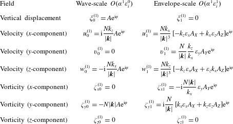
Expressions for different linear (in  $\unicode[STIX]{x1D6FC}$ ) fields (first column) at the scale of the waves (second column) and with small corrections (third column). This last column accounts for the finite but relatively large extent of the wavepacket in the $x$ , $y$ and $z$ directions, as prescribed through the values of $\unicode[STIX]{x1D700}_{x}$ , $\unicode[STIX]{x1D700}_{y}$ and $\unicode[STIX]{x1D700}_{z}$ , respectively (captured by $\unicode[STIX]{x1D700}_{i}$ in the column name). Values are given in terms of the amplitude envelope $A$ of the vertical displacement field, as found through the linearized equations for internal waves propagating in the $x$ – $z$ plane. It is understood that the actual fields are the real parts of the tabulated expressions, and the phase is given by $\unicode[STIX]{x1D711}=k_{x}x+k_{z}z-\unicode[STIX]{x1D714}t$ .

We introduce a second small parameter $\unicode[STIX]{x1D6FC}=|k_{x}|A_{0}$ , in which $A_{0}$ is the amplitude of vertical displacements at the centre of the group. At first order in $\unicode[STIX]{x1D6FC}$ , the vertical displacement field is given by

in which the superscript denotes the order in $\unicode[STIX]{x1D6FC}$ and the subscript denotes the order in the bandwidth parameters $\unicode[STIX]{x1D700}_{x}$ , $\unicode[STIX]{x1D700}_{y}$ and $\unicode[STIX]{x1D700}_{z}$ . As $\unicode[STIX]{x1D700}_{x}$ , $\unicode[STIX]{x1D700}_{y}$ and $\unicode[STIX]{x1D700}_{z}$ can be of different orders depending on the aspect ratio of the wavepacket that we later choose, we emphasize that the subscript does not play the role of a formal ordering parameter, but simply denotes the leading-order correction for the packet structure of the waves. The operator $\text{Re}[~]$ denotes taking the real part of the enclosed expression. For the vertical displacement field, we set higher-order terms in the bandwidth parameters to be zero without loss of generality. The second column of table 1 reports the usual polarization relationships for plane periodic internal waves, and the third column gives the next-order corrections accounting for the finite size of the wavepacket, which can be obtained from solving the linearized (in  $\unicode[STIX]{x1D6FC}$ ) governing equations (2.1).

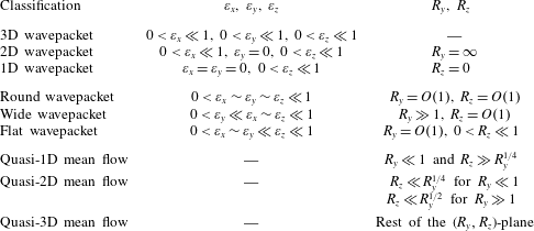
We also define the aspect ratios $R_{y}\equiv \unicode[STIX]{x1D70E}_{y}/\unicode[STIX]{x1D70E}_{x}$ and $R_{z}\equiv \unicode[STIX]{x1D70E}_{z}/\unicode[STIX]{x1D70E}_{x}$ . Table 2 formalizes the terminology used throughout the paper, distinguishing definitions based on the geometry of the wavepacket itself and definitions based on the nature and geometry of the induced flow. We will discuss the latter categorization in § 3.5 when we propose our regime diagrams. In the most general case of a three-dimensional (3D) wavepacket, the linear waves are modulated in all three directions, whereas a two-dimensional (2D) wavepacket is spanwise independent, as obtained by setting $\unicode[STIX]{x1D70E}_{y}\rightarrow \infty$ and thus $\unicode[STIX]{x1D700}_{y}\rightarrow 0$ . A one-dimensional (1D) wavepacket is not only spanwise independent or infinitely wide, but also periodic in the $x$ -direction, resulting in $\unicode[STIX]{x1D70E}_{x}\rightarrow \infty$ and thus $\unicode[STIX]{x1D700}_{x}\rightarrow 0$ . Such a 1D wavepacket is only modulated in the $z$ -direction. Approximately then, a 3D wavepacket is said to be ‘round’ when all three of its spatial scales are comparable: $0<\unicode[STIX]{x1D700}_{x}\sim \unicode[STIX]{x1D700}_{y}\sim \unicode[STIX]{x1D700}_{z}\ll 1$ . A 3D wavepacket is said to be ‘wide’ when its spanwise extent is larger than its ‘along-wave’ and vertical extents: $0<\unicode[STIX]{x1D700}_{y}\ll \unicode[STIX]{x1D700}_{x}\sim \unicode[STIX]{x1D700}_{z}\ll 1$ . Finally, a 3D wavepacket is said to be ‘flat’ when both its horizontal scales are comparable and larger than its vertical scale: $0<\unicode[STIX]{x1D700}_{x}\sim \unicode[STIX]{x1D700}_{y}\ll \unicode[STIX]{x1D700}_{z}\ll 1$ , corresponding to the definition in TA07.

Table 2.

Wavepacket- and induced-flow-based definitions. Note that the induced-flow-based definitions are subject to generalizations and restrictions discussed in § 3.5.

3.2 Mean-flow decomposition: Bretherton flow and long waves

It is evident from the outset that the solution to the mean-flow forcing equation (2.3) in combination with conservation of volume (2.1c ), a total of four equations, can give rise to three types of induced flows, leading to the classification into wavepackets that are effectively 1D (primarily inducing unidirectional flows), 2D (primarily inducing long-waves) and fully 3D (primarily inducing horizontally recirculating flows) (cf. table 2). The relative magnitudes of the three types of mean flow depend on the aspect ratios of the wavepackets. We first conceptually distinguish two contributions to the total mean flow of a wavepacket of general aspect ratio, namely the Bretherton flow (BF) and long waves (LW):

Writing the forcing in (2.3) as $\boldsymbol{F}=(F_{x},F_{y},F_{z})$ , we define the two components in (3.4) explicitly, so that

where the linear operator $\unicode[STIX]{x1D647}$ is defined in (2.3). Both components separately satisfy conservation of volume: $\unicode[STIX]{x1D735}\boldsymbol{\cdot }\boldsymbol{u}_{\mathit{BF}}=0$ and $\unicode[STIX]{x1D735}\boldsymbol{\cdot }\boldsymbol{u}_{\mathit{LW}}=0$ .

We begin in § 3.3 by deriving solutions for the well-known Bretherton flow, and consider the induced long waves in § 3.4. The method of inverse Fourier transforming, taking appropriate branch cuts to remove the singularity in the integrand, is also described in § 3.4. The total wave-induced mean flow is then given by the linear superposition of the two contributions, as defined in (3.4). We emphasize that we only consider up to second order in wave steepness $\unicode[STIX]{x1D6FC}$ and leading order in the separation-of-scales parameter $\unicode[STIX]{x1D700}$ , so that the effect of the mean flow on the nonlinear evolution of the wavepacket and the change in shape of the wavepacket due to dispersion, as considered by TA07, are beyond our scope. We return to this in § 5.

3.3 Bretherton flow

Taking the component of the total induced flow that is forced by the vertical vorticity of the linear waves (cf. (3.5a )), the Bretherton flow $\boldsymbol{u}_{\mathit{BF}}$ , we further decompose this flow as the sum of the divergent-flux-induced flow $\boldsymbol{u}_{\mathit{DF}}$ and the response flow $\boldsymbol{u}_{\mathit{RF}}$ :

The divergent-flux-induced flow is determined explicitly from the advection terms in the momentum equations (§ 3.3.1). The response flow is then found from conditions for incompressibility and irrotational flow (§ 3.3.2).

3.4 Long waves

Here, we consider the component of the total induced flow that is forced by the horizontal vorticity of the linear waves (cf. (3.5b )). We proceed with the following two assumptions. First, we assume that the induced flow has a much larger $x$ extent than that of the wavepacket itself motivated by considerations similar to the 2D (spanwise-infinite) case (cf. Bretherton Reference Bretherton1969; Tabaei & Akylas Reference Tabaei and Akylas2007; van den Bremer & Sutherland Reference van den Bremer and Sutherland2014). Explicitly, we let the induced long waves on the left-hand side vary horizontally on the new coordinate $\tilde{X}=\unicode[STIX]{x1D700}^{2}(x-c_{gx}t)$ . For a 2D wavepacket, Bretherton (Reference Bretherton1969) and van den Bremer & Sutherland (Reference van den Bremer and Sutherland2014) replace the forcing on the right-hand side by a Dirac delta function at the centre of the packet of equivalent strength by integrating with respect to $\tilde{x}$ between $\tilde{x}\rightarrow -\infty$ and $\tilde{x}\rightarrow \infty$ . As a consequence, any terms in the forcing that involve slow $x$ derivatives do not contribute. Second, we assume the wavepacket itself is relatively wide, $\unicode[STIX]{x1D700}_{y}\sim \unicode[STIX]{x1D700}^{2}$ , because a non-negligibly small contribution from the long waves is only expected then. Explicitly, we set $\unicode[STIX]{x1D700}_{z}=\unicode[STIX]{x1D700}$ and suppose $\unicode[STIX]{x1D700}_{y}\sim \unicode[STIX]{x1D700}^{2}$ in the linear operator on the left-hand side and in the forcing on the right-hand side of (2.3). Combining both assumptions, the wavepacket we examine is thus wide, but not necessarily flat (cf. TA07), as we set $\unicode[STIX]{x1D700}_{x}=\unicode[STIX]{x1D700}$ (or smaller) in the forcing on the right-hand side. From (2.3) and (3.5b ) we obtain

where we note that the averaging in (2.3) corresponds to averaging over the fast scales of waves within the wavepacket. It is evident that the entries in the final row, corresponding to operations acting on the vertical vorticity field, are of order $\unicode[STIX]{x1D700}^{4}$ . In order to have as many equations as unknowns after truncation at $O(\unicode[STIX]{x1D700}^{3})$ , we replace the final row by the incompressibility condition $\unicode[STIX]{x1D735}\boldsymbol{\cdot }\boldsymbol{u}_{\mathit{LW}}=0$ , which still needs to be satisfied.

The polarization relationships in table 1 allow for explicit evaluation of $(F_{x},F_{y},0)$ . From our first assumption above, we neglect terms involving slow $x$ derivatives because the response to the forcing is long compared to the wavepacket. We avoid the cumbersome operation of introducing Dirac delta functions, since neglecting terms involving slow $x$ derivatives leads to equivalent results. From our second assumption above, we neglect terms involving slow $y$ derivatives because the wavepacket is relatively wide. The terms involving $Z$ derivatives alone come from the product of the vertical velocity with the spanwise vorticity, each occurring at order $\unicode[STIX]{x1D6FC}$ . Thus, we find that the dominant forcing at $O(\unicode[STIX]{x1D6FC}^{2}\unicode[STIX]{x1D700}^{3})$ is

Combining these results, retaining terms up to $O(\unicode[STIX]{x1D700}^{3})$ , recasting the result in terms of the unscaled translating coordinate $(\tilde{x},{\tilde{y}},\tilde{z})$ and using (3.10), we have the following:

In the expression for the forcing on the right-hand side, we have used the equation for the vertical group velocity, $c_{gz}=-Nk_{x}k_{z}/|\boldsymbol{k}|^{3}$ . Next, we obtain the Fourier transform of (3.18), solve the resulting algebraic equations and then obtain the inverse Fourier transform. This gives the following general integral equation for the long-wave contribution to the wave-induced flow:

The singularity in the integrand of (3.19) corresponds to hydrostatic internal waves with wavenumber $(\unicode[STIX]{x1D705},\unicode[STIX]{x1D706},\unicode[STIX]{x1D707})$ set so that the vertical phase speed of the induced (long internal) waves equals the vertical group velocity of the wavepacket. It is the singularity in (3.19) that results in an induced flow with non-negligible vertical velocity. In order to select only outgoing waves, we make use of Cauchy’s residue theorem to integrate around the singularity in (3.19) and reduce the expression to a formula involving only a double integral (see also van den Bremer & Sutherland Reference van den Bremer and Sutherland2014). In order to apply the correct branch cut that selects only the outgoing waves, we switch to cylindrical coordinates in wavenumber space, defining $\unicode[STIX]{x1D703}$ so that $(\unicode[STIX]{x1D705},\unicode[STIX]{x1D706})=\unicode[STIX]{x1D705}_{H}(\cos \unicode[STIX]{x1D703},\sin \unicode[STIX]{x1D703})$ . Equation (3.19) becomes

where $\tilde{r}\equiv \sqrt{\tilde{x}^{2}+{\tilde{y}}^{2}}$ and $\unicode[STIX]{x1D703}_{p}\equiv \tan ^{-1}({\tilde{y}}/\tilde{x})$ . The singularity in (3.20) is split into two terms:

This expression in the integral can be decomposed into the sum of the Cauchy principal value and a Dirac delta function (see also Voisin Reference Voisin1991):

where the absolute value and sign of $\unicode[STIX]{x1D707}$ ensure outward-propagating waves. It is the delta function that gives rise to the radiating waves in the solution of the integral with respect to $\unicode[STIX]{x1D705}_{H}$ in (3.20):

in which $\unicode[STIX]{x1D705}_{H}=|c_{gz}|\unicode[STIX]{x1D707}^{2}/N$ in $\widehat{u_{\mathit{DF}}}$ . For $c_{gz}>0$ , the condition for outward-propagating waves requires $\unicode[STIX]{x1D707}\cos (\unicode[STIX]{x1D703}-\unicode[STIX]{x1D703}_{p})\geqslant 0$ , so that $\unicode[STIX]{x1D703}_{p}-\unicode[STIX]{x03C0}/2\geqslant \unicode[STIX]{x1D703}\geqslant \unicode[STIX]{x1D703}_{p}+\unicode[STIX]{x03C0}/2$ for $\unicode[STIX]{x1D707}\geqslant 0$ and $\unicode[STIX]{x1D703}_{p}+\unicode[STIX]{x03C0}/2<\unicode[STIX]{x1D703}<\unicode[STIX]{x1D703}_{p}+3\unicode[STIX]{x03C0}/2$ for $\unicode[STIX]{x1D707}<0$ (and vice versa for $c_{gz}<0$ ). Separately integrating over positive and negative $\unicode[STIX]{x1D707}$ and combining the results gives

Having removed the singularity, the double integral in (3.24) is readily solved by standard numerical integration techniques.

Equation (3.24) corresponds to the solution of the differential equation (31) in TA07 derived for flat wavepackets when neglecting rotation by setting the Coriolis parameter to zero. In our consideration of a wide, but not necessarily flat, wavepacket, the total induced mean flow corresponds to the sum of the Bretherton flow $\boldsymbol{u}_{\mathit{BF}}$ in (3.15) and the induced long waves $\boldsymbol{u}_{\mathit{LW}}$ in (3.24). Which of the two flows is dominant in the horizontal plane depends on the horizontal and vertical aspect ratios $R_{y}\equiv \unicode[STIX]{x1D70E}_{y}/\unicode[STIX]{x1D70E}_{x}=\unicode[STIX]{x1D700}_{x}/\unicode[STIX]{x1D700}_{y}$ and $R_{z}\equiv \unicode[STIX]{x1D70E}_{z}/\unicode[STIX]{x1D70E}_{x}=\unicode[STIX]{x1D700}_{x}/\unicode[STIX]{x1D700}_{z}$ . This is examined below in the specific case of a Gaussian wavepacket.

3.5 Dominant induced flows for different wavepacket aspect ratios

Although the equations above apply to any quasi-monochromatic wavepacket, here we specifically examine the predictions for Gaussian wavepackets with amplitude envelope $A=A_{0}\exp [-(\tilde{x}^{2}/\unicode[STIX]{x1D70E}_{x}^{2}+{\tilde{y}}^{2}/\unicode[STIX]{x1D70E}_{y}^{2}+\tilde{z}^{2}/\unicode[STIX]{x1D70E}_{z}^{2})/2]$ , in which $A_{0}$ is constant. Without loss of generality, we will assume that $A_{0}$ is real and positive, $k_{x}>0$ and $k_{z}<0$ , so that the vertical group velocity is positive. Our focus is to compare the largest values of the horizontal velocity associated with the Bretherton flow (3.15) with that associated with induced long waves (3.24): the former should be dominant for relatively round wavepackets (small  $\unicode[STIX]{x1D70E}_{y}$ ); the latter dominant for relatively wide wavepackets (large  $\unicode[STIX]{x1D70E}_{y}$ ).

From (3.10), we see that the largest magnitude of the divergent-flux-induced flow is $\Vert u_{\mathit{DF}}\Vert =N|\boldsymbol{k}||A_{0}|^{2}/2$ . Using (3.13), the Fourier-transformed divergent-flux-induced flow is $\widehat{u_{\mathit{DF}}}=[N|\boldsymbol{k}|\unicode[STIX]{x1D70E}_{x}\unicode[STIX]{x1D70E}_{y}\unicode[STIX]{x1D70E}_{z}/(16\unicode[STIX]{x03C0}^{3/2})]|A_{0}|^{2}\exp [-(\unicode[STIX]{x1D705}^{2}\unicode[STIX]{x1D70E}_{x}^{2}+\unicode[STIX]{x1D706}^{2}\unicode[STIX]{x1D70E}_{y}^{2}+\unicode[STIX]{x1D707}^{2}\unicode[STIX]{x1D70E}_{z}^{2})/4]$ . We substitute this into (3.15) and extract the largest value of the horizontal induced circulation of the Bretherton flow, which occurs at the centre of the wavepacket. Thus, we find the scaled maximum flow, $U_{\mathit{BF}}\equiv u_{\mathit{BF}}(0,0,0)/\Vert u_{\mathit{DF}}\Vert$ , to be (cf. § 14.3.3 of Bühler Reference Bühler2009)

in which $\hat{\unicode[STIX]{x1D705}}\equiv \unicode[STIX]{x1D705}\unicode[STIX]{x1D70E}_{x}$ , $\hat{\unicode[STIX]{x1D706}}\equiv \unicode[STIX]{x1D706}\unicode[STIX]{x1D70E}_{y}$ and $R_{y}\equiv \unicode[STIX]{x1D70E}_{y}/\unicode[STIX]{x1D70E}_{x}$ denotes the horizontal aspect ratio of the packet. This result is plotted as the thick solid line in figure 1(a).

Figure 1.

(a) Relative maximum value of the horizontal velocity and (b) its vertical location predicted as a function of the horizontal aspect ratio $R_{y}$ of the wavepacket for the Bretherton flow (solid line), induced long waves (blue dashed lines) and their combination (thick red dashed line). For values of $R_{y}$ for which our long-wave solution is not strictly valid, the blue dashed lines are replaced by blue dotted lines. Values are computed for a wavepacket with $k_{z}/k_{x}=-1$ and $\unicode[STIX]{x1D700}_{x}=\unicode[STIX]{x1D700}_{z}=1/5,1/20,1/100$ , as indicated ( $R_{z}=1$ ). The circles indicate the results measured from numerical simulations with $\unicode[STIX]{x1D700}_{x}=\unicode[STIX]{x1D700}_{z}=1/20$ and $R_{y}=1$ , 10, 40 and 100. The black diamond indicates the solution found for the numerical simulation of a 2D wavepacket by van den Bremer & Sutherland (Reference van den Bremer and Sutherland2014).

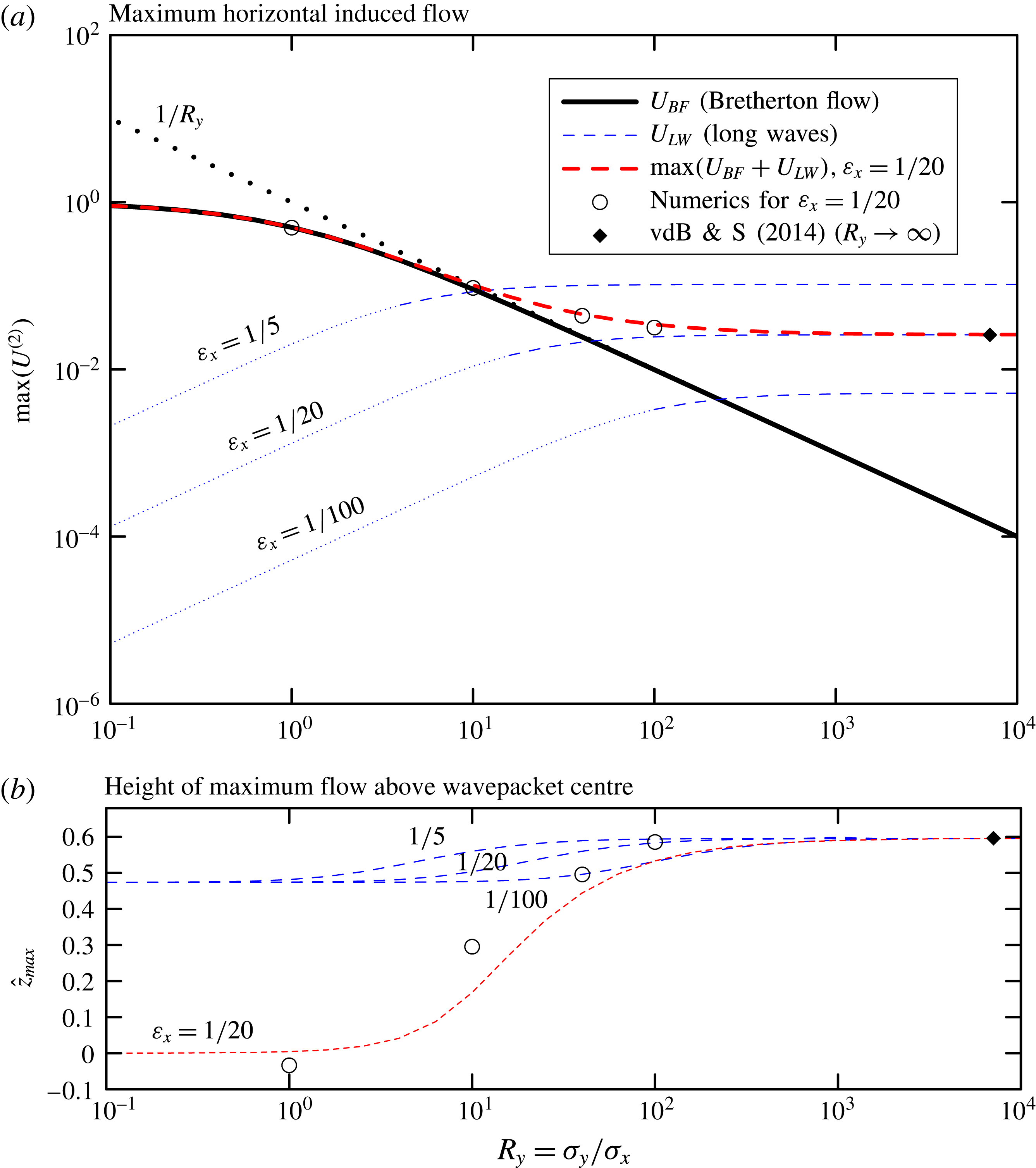
The induced long waves, on the contrary, have zero horizontal flow at the centre of the wavepacket, with the maximum in the streamwise direction occurring vertically above the centre. Defining the non-dimensional horizontal flow along the $\tilde{z}$ axis to be $U_{\mathit{LW}}(\hat{z})\equiv u_{\mathit{LW}}(0,0,\hat{z})/\Vert u_{\mathit{DF}}\Vert$ , we have, from (3.24),

in which $\hat{z}=\tilde{z}/\unicode[STIX]{x1D70E}_{z}$ and $K\equiv k_{x}^{2}|k_{z}|/|\boldsymbol{k}|^{3}$ . Consistent with the assumption that the generated waves are long relative to the $x$ extent of the packet, we can ignore the contribution $\unicode[STIX]{x1D705}^{2}\unicode[STIX]{x1D70E}_{x}^{2}/4=\unicode[STIX]{x1D705}_{H}^{2}\cos ^{2}(\unicode[STIX]{x1D703})\unicode[STIX]{x1D70E}_{x}^{2}/4$ in the envelope function $\widehat{u_{\mathit{DF}}}$ . The non-dimensional group $\unicode[STIX]{x1D6E5}$ plays the role of an effective wavepacket aspect ratio. For large $R_{y}$ , (3.26) reduces to its 2D equivalent (cf. (52) of van den Bremer & Sutherland Reference van den Bremer and Sutherland2014). For small $R_{y}$ , (3.26) corresponds to the wave field radiated by a point source in a 3D domain, noting the restriction that the packet remains wide (cf. § 3.4). How large $R_{y}$ has to be depends on the bandwidth parameter $\unicode[STIX]{x1D700}_{x}$ , the orientation of the wavevector $K$ and the aspect ratio $R_{z}$ , as captured by  $\unicode[STIX]{x1D6E5}$ .

We begin by considering the case for which $R_{z}=1$ : the wavepacket is round in the $x$ – $z$ plane, but of arbitrary width in the spanwise direction. The maximum and its relative vertical location are computed numerically and are plotted as a function of $R_{y}$ as the blue dashed lines in figure 1 for three different values of $\unicode[STIX]{x1D700}_{x}$ , as indicated; in both panels, we set $k_{z}=-k_{x}$ . It is worth emphasizing here that the long-wave contribution (3.26) is derived based on the assumption of a wide wavepacket: $\unicode[STIX]{x1D700}_{y}\sim \unicode[STIX]{x1D700}_{z}^{2}$ . Taking a practical approach, we thus set $\unicode[STIX]{x1D700}_{y}\leqslant \unicode[STIX]{x1D700}_{z}^{2}$ as its domain of validity, which corresponds to $R_{y}\geqslant R_{z}^{2}/\unicode[STIX]{x1D700}_{x}$ . For the values $\unicode[STIX]{x1D700}_{x}=\unicode[STIX]{x1D700}_{z}=1/5,1/20,1/100$ considered in figure 1, the dashed blue lines are thus only strictly valid for values of $R_{y}$ greater than 5, 20 and 100, as indicated by the transition of the blue dashed lines into blue dotted lines. It is evident that, for smaller values of $R_{y}$ , the magnitude of the long waves is sufficiently small compared to the Bretherton flow, so the long-wave contribution can be ignored regardless.

Figure 2.

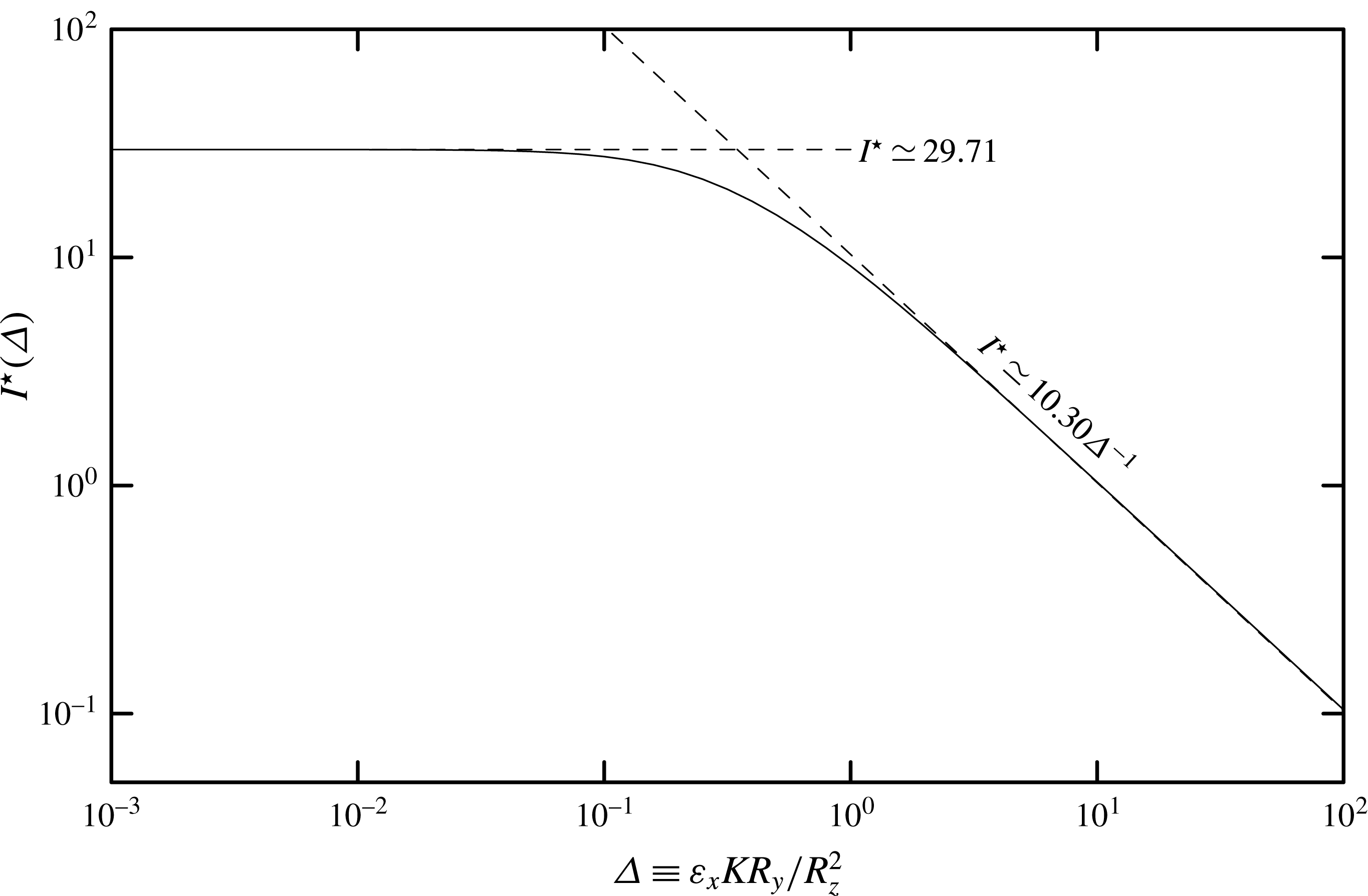
Maximum value of the double integral $I(\hat{z},\unicode[STIX]{x1D6E5})$ in (3.26) as a function of $\unicode[STIX]{x1D6E5}\equiv \unicode[STIX]{x1D700}_{x}KR_{y}/R_{z}^{2}$ . Asymptotic limits are indicated by the dashed lines: for $\unicode[STIX]{x1D6E5}\ll 0.1$ , $I^{\star }\sim 29.71$ ; for $\unicode[STIX]{x1D6E5}\gg 1$ , $I^{\star }\sim 10.30\unicode[STIX]{x1D6E5}^{-1}$ .

More generally, the asymptotic behaviour of $U_{\mathit{LW}}$ is determined first by finding the maximum, as it depends upon $\tilde{z}$ , of the double integral $I(\hat{z},\unicode[STIX]{x1D6E5})$ in (3.26), as a function of $\unicode[STIX]{x1D6E5}\equiv \unicode[STIX]{x1D700}_{x}KR_{y}/R_{z}^{2}$ . The resulting value, denoted by $I^{\star }(\unicode[STIX]{x1D6E5})$ , is plotted in figure 2. The double integral asymptotically approaches a constant value for small $\unicode[STIX]{x1D6E5}$ , and varies as $\unicode[STIX]{x1D6E5}^{-1}$ for large $\unicode[STIX]{x1D6E5}$ . The non-dimensional height where the maximum occurs varies only little, increasing from $\tilde{z}\simeq 0.474$ for small $\unicode[STIX]{x1D6E5}$ to $\tilde{z}\simeq 0.596$ for large $\unicode[STIX]{x1D6E5}$ . Taking a practical approach, the crossover from the small- to large- $\unicode[STIX]{x1D6E5}$ asymptotic regimes is estimated from the intersection of the two asymptotic curves, occurring for $\unicode[STIX]{x1D6E5}=\unicode[STIX]{x1D6E5}_{c}\simeq 0.35$ . Combining these results with the terms in front of the double integral in (3.26), we arrive at the following asymptotic approximations for the maximum induced flow in the $x$ -direction associated with induced long waves:

By comparing the maximum horizontal velocity of the Bretherton flow (3.25) and the limits of and the maximum horizontal velocity associated with induced long waves (3.27), we construct the regime diagram, shown in figure 3, which illustrates whether the flow induced by the wavepacket over its extent is best described by that of 1D, 2D or fully 3D wavepackets, as it depends upon the horizontal and vertical aspect ratios $R_{y}$ and $R_{z}$ . We will refer to these induced flows as quasi-1D, quasi-2D and quasi-3D and summarize the regimes in table 2. In order to draw boundaries to delineate what is a smooth transition between the different regimes, we make the following assumptions.

Figure 3.

Regime diagram indicating for what vertical and horizontal aspect ratios ( $R_{z}$ and $R_{y}$ , respectively) a Gaussian wavepacket will induce a flow similar to that of a 1D wavepacket (medium grey), a 2D wavepacket (light grey), which induces long waves, and a fully 3D wavepacket (white), which induces a horizontal circulation known as the Bretherton flow. The long-wave transition boundary is computed using (3.28) taking $|k_{z}|=|k_{x}|$ (so that $K=2^{-3/2}$ ) and $\unicode[STIX]{x1D700}_{x}=1/20$ . The cross-hatched regions indicate where the quasi-monochromatic wavepacket assumption breaks down for $\unicode[STIX]{x1D700}_{x}=1/20$ because either $\unicode[STIX]{x1D700}_{y}>1/5$ or $\unicode[STIX]{x1D700}_{z}>1/5$ . The region to the right of the dotted line corresponds to the domain of validity of the long-wave solution. The closed circles indicate the values of $R_{y}$ and $R_{z}$ for the five simulations with snapshots shown in figure 5.

A wavepacket is considered to be quasi-1D if the wave-induced flow has a magnitude within 10 % of the divergent-flux-induced flow $u_{\mathit{DF}}$ . From (3.25), this occurs for $R_{y}\lesssim 0.1$ . This transitional value is plotted as the vertical long-dashed line in figure 3.

A wavepacket is considered to be quasi-2D if the flow induced by long waves exceeds the Bretherton flow. An estimate of the critical vertical aspect ratio of the wavepacket $R_{z}^{\star }$ (as a function of $R_{y}$ ) when these flows are comparable is given by equating $U_{\mathit{BF}}$ in (3.25) to $U_{\mathit{LW}}$ in (3.27), in which the asymptotic approximations are extrapolated outside their strict domains of validity to $\unicode[STIX]{x1D6E5}=\unicode[STIX]{x1D6E5}_{c}$ . For $R_{y}\gtrsim 1.0$ , the large- $\unicode[STIX]{x1D6E5}$ limit dominates in (3.27). Otherwise the small- $\unicode[STIX]{x1D6E5}$ limit dominates. Together we find the transition boundary is given by

where the second similarity in two respective limits follows from taking the small- and large- $R_{y}$ limits of the $(1+R_{y})$ term. Equation (3.28) is plotted as the short-dashed curve in figure 3 for the case of a wavepacket with $|k_{z}|=|k_{x}|$ ( $K=2^{-3/2}$ ) and $\unicode[STIX]{x1D700}_{x}=1/20$ . In particular, for large $R_{y}$ and this choice of parameters, the transition curve between quasi-2D and quasi-3D wavepackets is given approximately by $R_{z}^{\star }\simeq 0.161R_{y}^{1/2}$ . Conversely, this transition written in terms of the horizontal aspect ratio as it depends upon the vertical aspect ratio is $R_{y}^{\star }\simeq [0.689/(K\unicode[STIX]{x1D700}_{x})]R_{z}^{2}\simeq 39.0R_{z}^{2}$ .

Evidently, it is worth emphasizing again that the long-wave contribution (3.26) is derived based on the assumption of a wide wavepacket and that its validity is thus limited to $R_{z}\leqslant \sqrt{\unicode[STIX]{x1D700}_{x}R_{y}}$ , denoted by the dotted line in figure 3. By equating the value of $R_{z}$ corresponding to this boundary to the transition value $R_{z}^{\star }$ in (3.28), we can obtain an estimate of how wide the wavepacket needs to be for our classification to be valid:

This is plotted in figure 4 as a function of the angle $\unicode[STIX]{x1D703}=\tan ^{-1}(|k_{z}/k_{x}|)$ that lines of constant phase make with the vertical. This minimum width is not dependent on $\unicode[STIX]{x1D700}_{x}$ . For the case $|k_{z}|=|k_{x}|$ considered herein, $\unicode[STIX]{x1D703}=45^{\circ }$ and $R_{y,min}=1.10$ . Our estimates in figure 3 are thus only valid for wavepackets that are at least marginally wider than they are long in the $x$ -direction, i.e. for $R_{y}\geqslant R_{y,min}=1.10$ .

Figure 4.

Minimum width for which the regime diagram is valid as a function of the angle $\unicode[STIX]{x1D703}$ that lines of constant phase make with the vertical ( $k_{x}=|\boldsymbol{k}|\cos (\unicode[STIX]{x1D703})$ ).

Finally, it is also important to keep in mind that these results rely on the starting assumption that the wavepacket is quasi-monochromatic, so that dispersion is a negligible effect. Hence all of $\unicode[STIX]{x1D700}_{x}$ , $\unicode[STIX]{x1D700}_{y}$ and $\unicode[STIX]{x1D700}_{z}$ must be much smaller than unity. For given $\unicode[STIX]{x1D700}_{x}$ , this puts a limitation on the aspect ratios $R_{y}=\unicode[STIX]{x1D70E}_{y}/\unicode[STIX]{x1D70E}_{x}=\unicode[STIX]{x1D700}_{x}/\unicode[STIX]{x1D700}_{y}$ and $R_{z}=\unicode[STIX]{x1D70E}_{z}/\unicode[STIX]{x1D70E}_{x}=\unicode[STIX]{x1D700}_{x}/\unicode[STIX]{x1D700}_{z}$ for which the transition boundaries can be considered reliable. In particular, the cross-hatched regions in figure 3 show the values of $R_{y}<5\unicode[STIX]{x1D700}_{x}$ and $R_{z}<5\unicode[STIX]{x1D700}_{x}$ for which the wavepacket is, respectively, too narrow ( $\unicode[STIX]{x1D700}_{y}>1/5$ ) or insufficiently tall ( $\unicode[STIX]{x1D700}_{z}>1/5$ ) for the case $\unicode[STIX]{x1D700}_{x}=1/20$ . The quasi-1D wavepacket regime and the long-wave regime in the small $R_{y}$ limit lie entirely within the cross-hatched regions for the value of $\unicode[STIX]{x1D700}_{x}$ considered here.

The different asymptotic regimes are summarized in table 2. In theory one could examine cases in which $\unicode[STIX]{x1D700}_{x}$ is so small that transitions to flows associated with 1D wavepackets and 2D wavepackets at small $R_{y}$ could be reliably predicted. However, in the numerical simulations that follow, we restrict our test of theory to the examination of wavepackets with $\unicode[STIX]{x1D700}_{x}=1/20$ . This is because simulations with significantly smaller $\unicode[STIX]{x1D700}_{x}$ would require much larger domain sizes and consequently more memory and longer computation time. Furthermore, vertically propagating wavepackets with $\unicode[STIX]{x1D70E}_{x}\gg 20k_{x}^{-1}\simeq 3\unicode[STIX]{x1D706}_{x}$ are unlikely to be generated by a realistic geophysical system on mesoscales and larger.

4.1 Code description

The flows induced by a Gaussian wavepacket were examined using fully nonlinear numerical simulations that solved the equations (2.1) with the addition of damping terms to the momentum and internal energy equations for the purpose of numerical stability. Specifically, under the assumption that $N^{2}$ is constant, the code evolved in time the horizontal velocity and vertical displacement fields according to

in which the vertical velocity $w$ and pressure divided by density $P\equiv p/\unicode[STIX]{x1D70C}_{0}$ were found from the respective diagnostic equations:

and

The equations were solved in Fourier space (corresponding to $x$ , $y$ and $z$ ) in a triply periodic domain. The nonlinear (e.g. advective) terms in the equations were computed by fast Fourier transforming the fields to real space, multiplying and then transforming back to Fourier space. The diffusion operator ${\mathcal{D}}$ was prescribed to act as a Laplacian operator only upon horizontal wavenumbers greater than $2k_{x}$ . The diffusivities of momentum and substance acting on these high wavenumbers were set to be $\unicode[STIX]{x1D708}=\unicode[STIX]{x1D705}=0.001N/k_{x}^{2}$ . The fields were advanced in time using a leapfrog scheme with an Euler backstep taken every 20 steps.

4.2 Initial conditions

The initial wavepacket centred at the origin had wavenumber set so that $k_{z}=-k_{x}$ , and the Gaussian envelope had amplitude $A_{0}=0.01/k_{x}$  ( $\unicode[STIX]{x1D6FC}=0.01$ ) and $x$ extent $\unicode[STIX]{x1D70E}_{x}=20/k_{x}$  ( $\unicode[STIX]{x1D700}_{x}=1/20$ ). The details of the five simulations presented here are summarized in table 3. We first examined four vertically round ( $\unicode[STIX]{x1D70E}_{z}=\unicode[STIX]{x1D70E}_{x}$ , $R_{z}=1$ ) wavepackets with lateral extents $k_{x}\unicode[STIX]{x1D70E}_{y}=20$ , 200, 800 and 2000, thus exploring the range between round and wide wavepackets with $R_{y}=1$ , 10, 40 and 100, bracketing the predicted critical transition value of $R_{y}^{\star }=39.0$ , as derived below (3.28). Furthermore, we examined a more flat wavepacket chosen to lie on our transition curve in figure 3 ( $R_{y}=10$ , $R_{z}=0.5$ ).

Table 3.

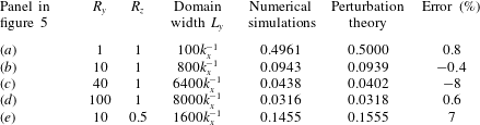
Comparison of the scaled maximum horizontal velocity $U^{(2)}$ from numerical simulations and perturbation theory.

The choice of initial conditions for the mean flow is crucial for the interpretation of results from numerical simulations. Up to the orders we consider (see also § 5), our analytical solution consists of a packet that translates at the group velocity, and the mean flow (Bretherton flow and long waves) it induces is entirely steady. Numerical solutions intended to reproduce this steady solution should therefore in principle have both aspects, the linear packet and the second-order mean flow (Bretherton flow and long waves), superimposed at the outset. If the second-order solutions are not superimposed at the outset, the flow responds as follows. The second-order (amplitude) equations instantaneously demand the generation of a mean flow (Bretherton flow and long waves) that are bound to the packet and travel with it. An ‘error wave’ (or flow) then forms that is equal and of opposite sign to the mean flow, so that the total second-order signal is zero, as prescribed by the initial conditions and by conservation of momentum. The error wave does not generally travel at the same speed as the packet. Here, it stays behind. The error wave can be thought of as unphysical in the sense that it is not part of a (quasi-)steady solution. If one is interested in this (quasi-)steady solution, it is imperative to wait long enough for the solution and the error wave to separate (cf. van den Bremer & Sutherland Reference van den Bremer and Sutherland2014).

Here, we take the following practical approach. Out of the two parts of the second-order mean flow (the Bretherton flow and the long waves), we have only initialized with the Bretherton flow predicted by (3.15). This way, we do not leave an error flow (with opposite sign to the Bretherton flow) behind and can see whether waves are indeed generated, but we do leave behind error waves (with opposite sign to the long waves). We are left with the subtlety that the long waves will consist of both the actual long waves travelling with the packet and the error wave left behind. We will have to wait for long enough for the two to separate, conceptually analogous to what was done by van den Bremer & Sutherland (Reference van den Bremer and Sutherland2014).

4.3 Domain size and post-processing

In all cases, the domain was set to be much larger than the anticipated spatial extent of the induced flow over the duration of the simulation, up to time $t=200/N$ when the wavepacket had propagated sufficiently far away from its initial position centred at the origin. The simulation resolved disturbances with wavenumbers up to $4k_{x}$ and $4|k_{z}|$ in the $x$ - and $z$ -directions. In the case $R_{y}=1$ , the spanwise domain range was $|y|\leqslant L_{y}$ with $L_{y}=100k_{x}^{-1}$  ( $k_{z}=-k_{x}$ ) and resolved by wavenumbers up to $128\unicode[STIX]{x03C0}/L_{y}$ . In the wider cases, the domain was substantially larger to accommodate the generation of long waves and so the resolution was reduced in order for the numerical simulations to complete in a reasonable time frame (see table 3), with wavenumbers being resolved up to $32\unicode[STIX]{x03C0}/L_{y}$ . The time resolution was $0.010/N$ in the case $R_{y}=1$ and $0.025/N$ in the cases $R_{y}=10$ , 40 and 100. Each run took four days to complete running in serial on a 2.9 GHz Intel Core i5.

The flows induced by the wavepacket were assessed by filtering the Fourier modes with horizontal wavenumbers between $0.5k_{x}$ and $2k_{x}$ corresponding to the linear waves that make up the wavepacket. The inverse transform thereby revealed the flow induced by the propagating wavepacket. The result of this analysis at the end of five simulations is shown in figure 5, which plots cross-sections of the $x$ -component of the induced flow at time $t=200/N$ , when the wavepacket had propagated sufficiently far away from its initial position at the origin, being centred at $(x,y,z)\simeq (70.7,0,70.7)$ . (A multimedia version of figure 5 is available online at https://doi.org/10.1017/jfm.2017.745, which shows 3D representations of the induced flows and their cross-sections.)

Figure 5.

The wavepacket-filtered $x$ -component of velocity determined at time $Nt=200$ from five simulations initialized with a Gaussian wavepacket of maximum amplitude $A_{0}=0.01k_{x}^{-1}$ centred at the origin, having vertical wavenumber $k_{z}=-k_{x}$ , $x$ extents of $\unicode[STIX]{x1D70E}_{x}=20k_{x}^{-1}$ , and $y$ and $z$ extents as reported in the panels. The left (right) panels show a cross-section of the flow in the $y$ – $z$ ( $x$ – $z$ ) plane through the centre of the wavepacket. The thick black ovals are drawn around one standard deviation from the centre of the wavepacket predicted to be at $(c_{gx}t,0,c_{gz}t)$ ; these ovals appear as vertical lines in the right panels of (b)–(e) because the extents in $x$ are small compared to the width of the domain. The colour bars to the lower left in the left panels indicate the magnitude of the induced flows in the left and corresponding right panels.

5.1 Round wavepackets

If the modulations are equally strong in all three directions and indeed as strong as the effect of rotation, TA07 also conclude that the velocity is essentially horizontal (their § 2.1). Without making restrictive assumptions about the amplitude of the waves, the mean flow is then governed by their (17) and (18), which is in agreement with Grimshaw (Reference Grimshaw1972) in the absence of rotation, as noted by these authors. Without rotation and in the weakly nonlinear limit, their (17) and (18) reduced to their (22), which in turn agrees with Shrira (Reference Shrira1981) (and Bretherton Reference Bretherton1969), as noted by TA07. In the small-amplitude limit, our prediction given by (3.14) is the solution to (22) in TA07.

The right panel of our figure 5(a) can be compared at least qualitatively with the induced flow shown by line contours in the left panel of figure 4 of TA07. Their simulation was somewhat different: it included the effects of rotation, and the vertical wavenumber was relatively smaller in magnitude. Despite these differences, two instructive comparisons can be made. First, because TA07 did not initialize the simulation with the predicted Bretherton flow, they observe a negative, non-translating, induced flow at the origin in addition to the positive induced flow that translates with the wavepacket. Second, because their wavepacket was round in this simulation, TA07 also did not observe the generation of long waves. Our figure 1 indeed confirms that the maximum induced flow associated with long waves is three orders of magnitude smaller than the Bretherton flow in the case $R_{y}=1$ and $\unicode[STIX]{x1D700}_{x}=1/20$ (and $R_{z}=1$ ).

5.2 Flat wavetrains

Assuming the horizontal extent of the wavepacket is comparable in the $x$ - and $y$ -directions but both are much larger than the vertical extent, TA07 predicted the wavepacket should excite long waves according to their (31). They solved this prognostic differential equation in a simulation with no rotation, setting $|k_{z}/k_{x}|=0.4$ (so $K=0.32$ ), and setting the horizontal wavepacket extent in both directions to be 100 times larger than the vertical extent indeed shows trailing waves (so $R_{y}=1$ , $R_{z}=0.01$ and $\unicode[STIX]{x1D700}_{x}=10^{-4}$ ). This indeed showed the generation of trailing long waves, as revealed in figure 2 of TA07. Yet evidence of an induced flow at the origin is indicative of an error flow resulting from not superimposing the predicted induced flow at the outset and thus considering an inherently unsteady problem.

Generally, we predict that a flat wavepacket should excite long waves of comparable or larger amplitude than the Bretherton flow if $R_{z}\lesssim R_{z}^{\star }$ , with $R_{z}^{\star }$ given by (3.28). With $R_{y}=1$ , $K=0.32$ and $\unicode[STIX]{x1D700}_{x}=10^{-4}$ , we predict the transition occurs at $R_{z}^{\star }\simeq 0.007$ . Thus, the simulation of TA07 shown in their figure 2 corresponds to the regime of induced flows dominated by the Bretherton flow, but which is nonetheless close to the transition in which induced long waves have comparable amplitude. This explains the appearance of the Bretherton-flow-like error flow at the origin as well as the manifestation of induced long waves trailing the propagating wavepacket.