1 Introduction
The clustering of inertial particles in turbulence is important in a broad spectrum of natural, biomedical and industrial processes, including sediment transport, cloud formation, planetary accretion, aerosol inhalation, and spray combustion. It is indeed well known that particles in turbulent flows exhibit non-uniform spatial distributions; a phenomenon highly dependent on the particle Stokes number, defined as the ratio of the aerodynamic particle response time to the characteristic fluid time scale. Since the pioneering work of Maxey (Reference Maxey1987), many early studies have found evidence that heavy particles are centrifuged out of high-vorticity regions of the flow, causing them to preferentially concentrate in the high-strain regions between vortices (Squires & Eaton Reference Squires and Eaton1991; Elghobashi & Truesdell Reference Elghobashi and Truesdell1992). More recent studies have proposed alternative mechanisms to explain the non-uniform particle concentration (Goto & Vassilicos Reference Goto and Vassilicos2008; Bragg & Collins Reference Bragg and Collins2014), but its manifestation has not been disputed. Notable consequences of this behaviour include the enhancement of particle collision rates (Sundaram & Collins Reference Sundaram and Collins1997; Wang, Wexler & Zhou Reference Wang, Wexler and Zhou2000) and the increase in settling velocity (Wang & Maxey Reference Wang and Maxey1993; Aliseda et al. Reference Aliseda, Cartellier, Hainaux and Lasheras2002).
An additional, seemingly obvious consequence of the increased local concentration is the formation of particle clusters. In their recent review, Monchaux, Bourgoin & Cartellier (Reference Monchaux, Bourgoin and Cartellier2012) defined clusters as ‘groups of particles that remain close to one another (and possibly interact) on time scales long compared to some turbulence time scale’, and further called them ‘dynamical evolutive entities implying possible collective effects’. Indeed, when a relatively large number of particles accumulate, their dynamics (and not only their kinematics) may become important: even if individual particles carry negligible momentum, their collective action on the carrier fluid can be locally significant (two-way coupling), as well as the interaction with neighbouring particles (four-way coupling) (Elghobashi Reference Elghobashi1994). While the existence of clusters is believed to be important for virtually all processes where preferential concentration takes place, a clear topological definition of clusters has been lacking, limiting our ability to describe their features and dynamics.
Several approaches have been taken to characterize clustering in particle distributions; here we mention just the most common. The box-counting method consists in dividing the domain into boxes of equal size, counting the particles in each box, and comparing the probability density function (PDF) of the number of particles per box against the Poisson distribution typical of randomly distributed particles. This technique provides a simple scalar measure of the amount of clustering and has been successfully used in experimental studies (Kulick, Fessler & Eaton Reference Kulick, Fessler and Eaton1994; Aliseda et al. Reference Aliseda, Cartellier, Hainaux and Lasheras2002). Its main drawback is that it introduces an extrinsic and arbitrary length scale (the box size). The radial distribution function (RDF) describes the probability of finding a particle at a certain distance away from another one, and represents the most widely used tool to quantify turbulence-driven clustering of particles and droplets (Sundaram & Collins Reference Sundaram and Collins1997; Kostinski & Shaw Reference Kostinski and Shaw2001; Wood, Hwang & Eaton Reference Wood, Hwang and Eaton2005; Saw et al. Reference Saw, Shaw, Ayyalasomayajula, Chuang and Gylfason2008; Gualtieri, Picano & Casciola Reference Gualtieri, Picano and Casciola2009; Zaichik & Alipchenkov Reference Zaichik and Alipchenkov2009). This method is powerful in that it provides a scale-by-scale quantification of clustering, and it lies at the core of statistical collision models (Wang et al. Reference Wang, Wexler and Zhou2000). However, the RDF gives global rather than local information, as it is typically computed over the whole particle field without identifying individual clusters.
Monchaux, Bourgoin & Cartellier (Reference Monchaux, Bourgoin and Cartellier2010) introduced the use of Voronoï diagrams to the field of particle-laden turbulence: the domain is divided into cells associated to each individual particle, with each cell containing the set of points closer to that particle than to any other. The inverse of the volume of each cell is equal to the local particle concentration, which is therefore naturally defined at a spatial resolution intrinsic to the local particle distribution. Another advantage is that the Voronoï diagram can be computed very efficiently, even on large sets of particles. This approach has recently encountered wide favour, and several authors have used it to analyse inertial particle fields in experimental (Obligado et al. Reference Obligado, Teitelbaum, Cartellier, Mininni and Bourgoin2014; Rabencov & van Hout Reference Rabencov and van Hout2015) and numerical studies (Tagawa et al. Reference Tagawa, Mercado, Prakash, Calzavarini, Sun and Lohse2012; Dejoan & Monchaux Reference Dejoan and Monchaux2013; Kidanemariam et al. Reference Kidanemariam, Chan-Braun, Doychev and Uhlmann2013; Nilsen, Andersson & Zhao Reference Nilsen, Andersson and Zhao2013). These have spanned one-way and two-way coupled regimes, with both point-like and finite-size particles. Recent studies have used both RDFs and Voronoï diagrams to characterize highly coupled systems in which the particles absorb radiative heat and release it to the fluid (Zamansky et al. Reference Zamansky, Coletti, Massot and Mani2016; Pouransari & Mani Reference Pouransari and Mani2017). Besides methods that evaluate the instantaneous particle field, several authors have used direct or kinematic simulations to investigate the Lagrangian particle dynamics, and in particular the rate at which nearby particles separate or approach each other (Falkovich & Pumir Reference Falkovich and Pumir2004; Ijzermans, Meneguz & Reeks Reference Ijzermans, Meneguz and Reeks2010; Esmaily-Moghadam & Mani Reference Esmaily-Moghadam and Mani2016, among others). By analysing the deformation and number density of the particle field along particle trajectories, these approaches have shed light on how clustering relates to the underlying flow.
Both the box-counting method and the Voronoï diagram method have been used to identify individual clusters (as well as voids, i.e. regions depleted of particles); see, for example, Aliseda et al. (Reference Aliseda, Cartellier, Hainaux and Lasheras2002), Goto & Vassilicos (Reference Goto and Vassilicos2006), Monchaux et al. (Reference Monchaux, Bourgoin and Cartellier2010), Obligado et al. (Reference Obligado, Teitelbaum, Cartellier, Mininni and Bourgoin2014), Zamansky et al. (Reference Zamansky, Coletti, Massot and Mani2016). The strategy has been to establish a maximum box or cell volume (i.e., a minimum concentration) threshold, and to define as cluster the set of particles belonging to the same connected group of boxes or cells whose volume is below the threshold. To avoid spurious edge effects, the additional condition is sometimes applied that the volume of the neighbouring cells of the particle must also be smaller than the threshold.
Starting from the Voronoï diagram method, we introduce here a definition of coherent cluster based on self-similarity, and apply it to the distribution of inertial particles in homogeneous isotropic turbulence obtained by direct numerical simulations (DNS). We consider a range of particle Stokes numbers, with and without the effect of gravity. By applying this definition, we identify individual clusters, and characterize their topology and kinematics in the turbulent flow, focusing our attention on the one-way coupled regime. The paper is organized as follows: in § 2 we describe the numerical method and summarize the investigated cases; in § 3 we illustrate the procedure for the identification of coherent clusters; in § 4 we present the results in terms of cluster topology, behaviour, and clustered-conditioned flow statistics; the conclusions and an outlook for further research are provided in § 5.
2 Method
The simulations are carried out using the same numerical set-up described in Pouransari, Mortazavi & Mani (Reference Pouransari, Mortazavi and Mani2015) and Frankel et al. (Reference Frankel, Pouransari, Coletti and Mani2016), which investigated particle–fluid transfer of momentum and heat, but with several simplifications: the system is isothermal, and the momentum back-reaction of the particles on the fluid is neglected. We therefore limit our attention to the momentum one-way coupling between hydrodynamic turbulence and inertial point particles. The Navier–Stokes equations are solved using a staggered grid formulation and second-order central finite differences. Particles are individually tracked along their trajectories, according to the simplified particle equation of motion where only contributions from Stokes drag and gravity are retained. Both the fluid and particle equations are integrated in time using a fourth-order Runge–Kutta scheme. The initial conditions are generated from a Passot–Pouquet spectrum with the particles distributed randomly in space. The turbulence is maintained using a linear forcing method (Lundgren Reference Lundgren2003; Rosales & Meneveau Reference Rosales and Meneveau2005). The domain is a triply periodic cube of size
 ${\mathcal{L}}=0.237$
m, which is uniformly discretized in
 $256^{3}$
grid points and populated with approximately four million particles. The discretization is sufficient to resolve all scales of the turbulence, with the grid spacing being approximately equal to
 $1.5\unicode[STIX]{x1D702}$
. The domain size and the number of particles are chosen to limit the computational effort in performing both the numerical simulations and the Voronoï cluster analysis, which includes the tessellation and connectivity information for the several considered cases. Further details on the numerical implementation can be found in Frankel et al. (Reference Frankel, Pouransari, Coletti and Mani2016).
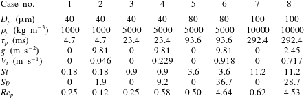
Fluid phase physical parameters.

Particle phase physical parameters.
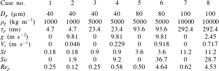
The main parameters for the continuum and dispersed phase are listed in tables 1 and 2, respectively. The fluid properties approximate air at standard temperature and pressure. In each case, statistics are taken from 20 independent realizations obtained after the system has become stationary. For all simulations, the Taylor microscale Reynolds number is
 $Re_{\unicode[STIX]{x1D706}}=65$
. The integral length and time scales are
 $L=u_{RMS}^{3}/\unicode[STIX]{x1D700}$
and
 $T=L/u_{RMS}$
, respectively,
 $u_{RMS}$
being the r.m.s. velocity fluctuation and
 $\unicode[STIX]{x1D700}$
the turbulent dissipation rate. Strictly, in the present one-way coupled point-particle approach, the particles do not possess a finite size and the only physical parameter relevant to the simulations is the aerodynamic response time. However, we have chosen the latter based on realistic values for the size and density of the particles. We consider different combinations of particle size (
 $D_{p}$
) and density (
 $\unicode[STIX]{x1D70C}_{p}$
) and gravitational acceleration (
 $g$
), resulting in eight combinations of the Stokes number
 $St\equiv \unicode[STIX]{x1D70F}_{p}/\unicode[STIX]{x1D70F}_{\unicode[STIX]{x1D702}}$
and settling parameter
 $Sv\equiv V_{t}/u_{\unicode[STIX]{x1D702}}$
. Here
 $\unicode[STIX]{x1D70F}_{p}$
is the particle aerodynamic response time,
 $\unicode[STIX]{x1D70F}_{\unicode[STIX]{x1D702}}$
and
 $u_{\unicode[STIX]{x1D702}}$
are the Kolmogorov time and velocity scales, respectively, and
 $V_{t}=\unicode[STIX]{x1D70F}_{p}g$
is the still-fluid settling velocity.
 $D_{p}$
is considerably smaller than the Kolmogorov length scale
 $\unicode[STIX]{x1D702}$
, and for most cases the particle Reynolds number
 $Re_{p}$
(based either on the settling velocity or on the r.m.s. fluid velocity fluctuation) is smaller than one, justifying (to first approximation) the assumption of Stokesian drag. Cases no. 6 and no. 8 have relatively fast-settling particles, and consequently
 $Re_{p}$
is larger than unity. However, we choose not to correct for the nonlinear drag, as this allows us to focus on the fundamental (although idealized) point-particle kinematics. Therefore, considering the high particle-to-fluid density ratios, the aerodynamic response time is calculated for all cases as
 $\unicode[STIX]{x1D70F}_{p}=\unicode[STIX]{x1D70C}_{p}D_{p}^{2}/18\unicode[STIX]{x1D707}$
, where
 $\unicode[STIX]{x1D707}$
is the dynamic viscosity. The combinations of parameters are chosen so as to explore a range of regimes in which preferential concentration, clustering, and altered settling are expected, while using realizable physical properties. Notice that in most simulations the acceleration field is
 $g_{0}=9.81~\text{m}~\text{s}^{-2}$
, except in case no. 8 in which we use
 $g=g_{0}/4$
. This reduced gravitational acceleration allows us to consider relatively high Stokes particles (
 $St=11.2$
) without incurring spurious periodicity effects due to the limited size of the domain (Ireland, Bragg & Collins Reference Ireland, Bragg and Collins2016). Case no. 8 is also relevant to the conditions found elsewhere in the solar system.
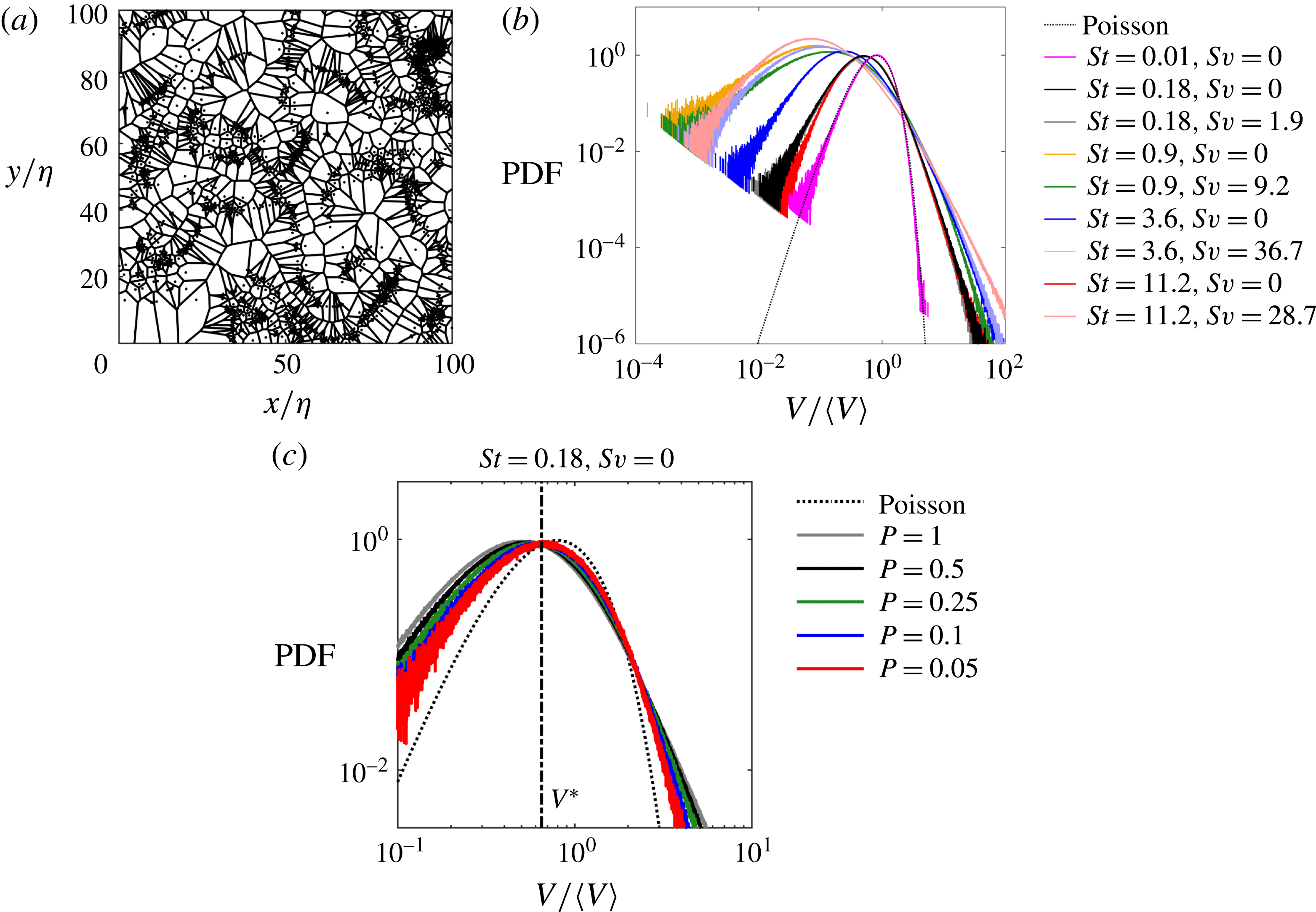
Two-dimensional Voronoï tessellation of a slice of thickness
 $2\unicode[STIX]{x1D702}$
from the
 $St=0.9$
,
 $Sv=0$
case (a), PDFs of the Voronoï cell volume V normalized by the mean cell volume
 $\langle V\rangle$
for each case compared with the
 $\unicode[STIX]{x1D6E4}$
distribution expected of a Poisson random process (b), and PDFs of Voronoï cell volume of the
 $St=0.18$
,
 $Sv=0$
case for subsamples of fraction P of the full set of particles (c). The volume threshold
 $V^{\ast }$
is marked with a vertical dash-dotted line.

3 Cluster identification
The method we propose to identify individual particle clusters is based on the Voronoï diagram approach, although it can also be implemented using other tessellation methods, e.g. the box-counting method. As mentioned in § 1, the Voronoï diagram method has specific merits, in particular the fact that a concentration threshold for a particle to belong to a cluster is intrinsic to the distribution, rather than chosen a priori. This is illustrated in figure 1, picturing an instantaneous distribution of particles and the corresponding Voronoï tessellation from one of our simulations, as well as the PDF of the cell volumes V for the various considered cases. The volumes are normalized by the average cell volume
 $\langle V\rangle$
, equal to the inverse of the mean concentration. The Voronoï cell distribution (figure 1
b) is consistent with previous studies that investigated comparable physical parameters, see, for example, Dejoan & Monchaux (Reference Dejoan and Monchaux2013). Comparing against the
 $\unicode[STIX]{x1D6E4}$
distribution expected for a set of randomly distributed particles (Ferenc & Néda Reference Ferenc and Néda2007), the intersection
 $V^{\ast }$
defines a volume threshold (equivalently, a concentration threshold) below which particles may be considered clustered (Monchaux et al.
Reference Monchaux, Bourgoin and Cartellier2010). That is, compared to randomly distributed fluid tracers, the inertial particles have a higher chance to be found at local concentrations higher than
 $1/V^{\ast }$
, and therefore to be associated to cells smaller than
 $V^{\ast }$
. We include the PDF of Voronoï cell volumes for a case at a vanishingly small Stokes number in figure 1(b) to show that the distribution of these tracer particles does indeed overlap with the
 $\unicode[STIX]{x1D6E4}$
distribution. We remark that the condition
 $V<V^{\ast }$
is necessary but not sufficient for a particle to belong to a cluster. The Voronoï diagram method has proven to be fairly robust to potential biases related to a considered data set. In particular, Monchaux et al. (Reference Monchaux, Bourgoin and Cartellier2012) showed that, by removing 40 % of the particles in the domain, the behaviour of the standard deviation of the Voronoï volume distributions for different Stokes number was preserved, while the absolute values were decreased by at most 25 %. Crucial for the present study is that, as shown in figure 1(c), the threshold
 $V^{\ast }$
is essentially unaffected by particle subsampling: analysing a fraction P of the four million particles in the domain shows no quantitative change even at fractions as low as
 $P=0.05$
.
In previous studies the next and final step to recognize individual clusters is to consider particles associated to connected sets of Voronoï cells with volume
 $V<V^{\ast }$
. However, by applying this condition only, one may also identify as clusters random collections of even a few particles which happen to be close to each other. While this might be acceptable from a geometric standpoint, our understanding of preferential concentration suggests that turbulence-driven clusters should have topological features reflecting the dynamics of the underlying flow. In particular, turbulent fields have been shown to possess various degrees of self-similarity and to exhibit fractal properties (Sreenivasan Reference Sreenivasan1991; Moisy & Jiménez Reference Moisy and Jiménez2004; de Silva et al.
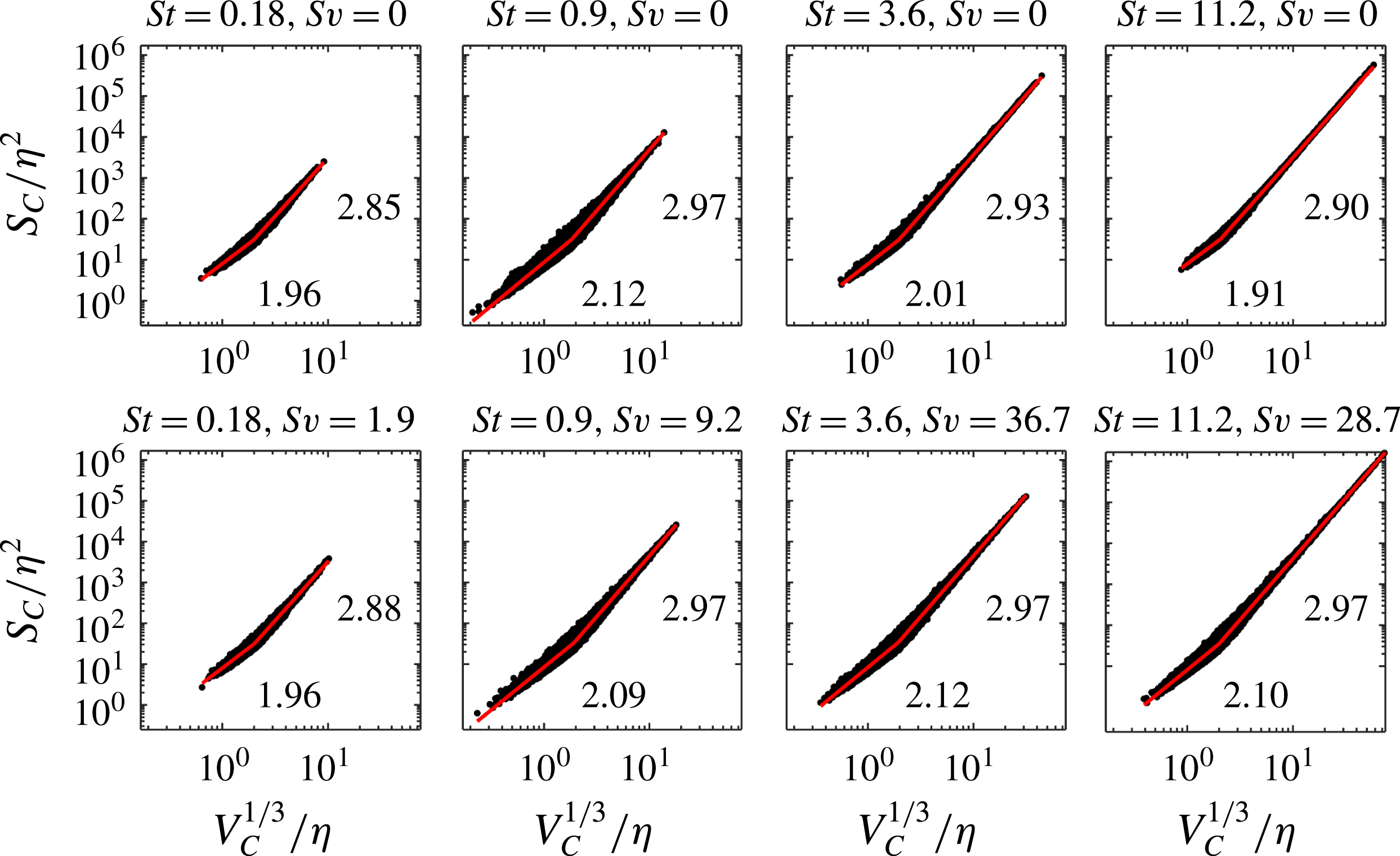
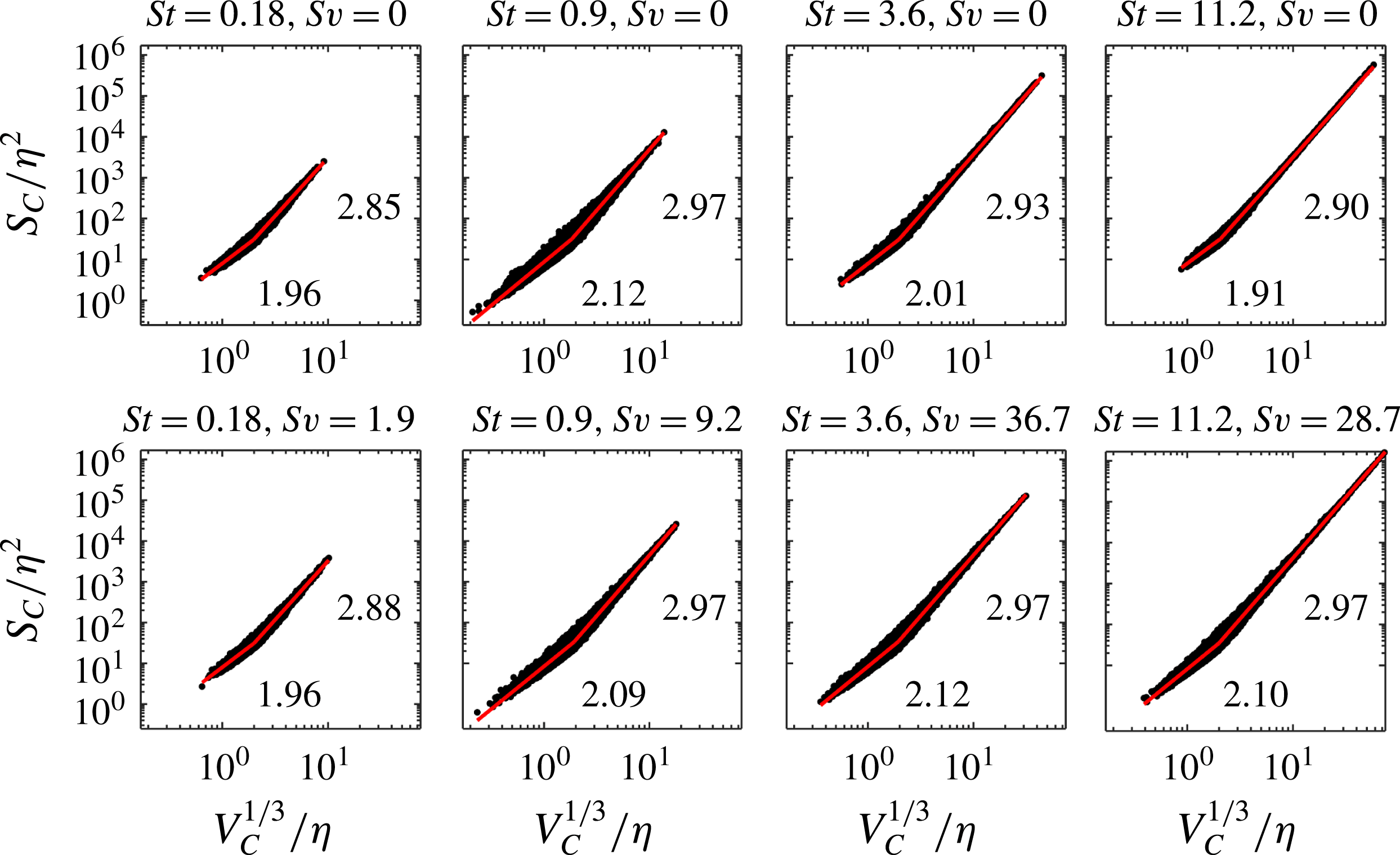
Reference de Silva, Philip, Chauhan, Meneveau and Marusic2013, among others). Inertial particles in turbulence have also been shown to follow self-similar distributions, with the size PDF of the voids between clusters displaying a clear power-law decay (Goto & Vassilicos Reference Goto and Vassilicos2006; Yoshimoto & Goto Reference Yoshimoto and Goto2007) for two-dimensional and three-dimensional turbulence, respectively. In our identification process, we therefore impose the further restriction that the clusters be large enough to display self-similarity. To this end, we consider the sets of connected Voronoï cells associated to each cluster and analyse the relation between the set surface area,
 $S_{C}$
, and the cubic root of the set volume,
 $V_{C}$
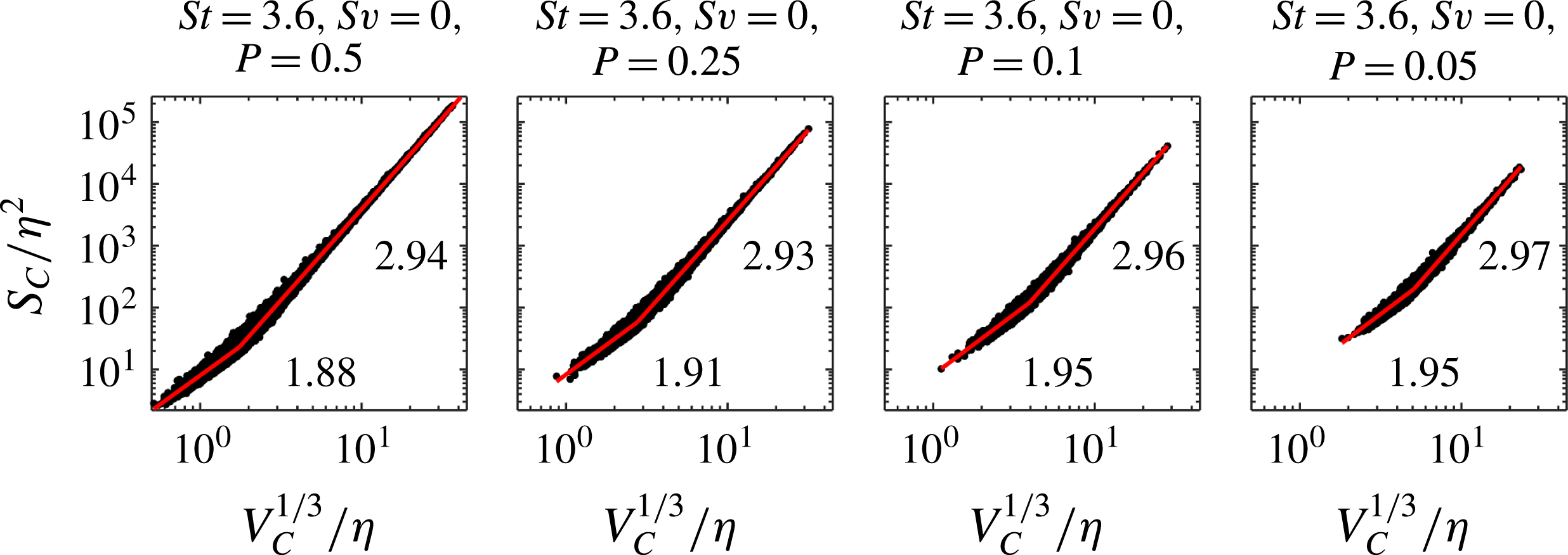
. (In the following we will refer to ‘cluster surface area’ and ‘cluster volume’, although these are strictly properties of the connected set of Voronoï cells associated to the particles in each cluster.) Figure 2 shows scatter plots of these quantities (normalized by the Kolmogorov scale) for each of the eight investigated cases. For small clusters, the relationship follows a power law with an exponent of approximately 2 (expected for regular three-dimensional objects), while for larger clusters the exponent is 2.85 or higher, indicating a fractal structure of their surrounding surface. In Kolmogorov scaling, the boundary between fractal and non-fractal behaviour corresponds to cluster volumes between
 $(1.9\unicode[STIX]{x1D702})^{3}$
and
 $(2\unicode[STIX]{x1D702})^{3}$
for all cases. We conventionally chose
 $8\unicode[STIX]{x1D702}^{3}$
as the threshold above which clusters are considered significant. By this choice we mean that clusters in this class are likely brought together by coherent structures of the turbulent velocity field, and therefore their presence and features are directly related to the nature of the flow. In the present one-way coupled simulations we investigate only their position and velocity (i.e. their kinematics) in relation with the flow topology; we cannot explore the back-reaction that clustered particles exert, individually or collectively, on the flow (i.e. their dynamics). However, as we will discuss further in § 5, because the coherent clusters have relatively high concentration over regions of space larger than the viscous scales of the flow, they appear likely to play a significant role in the fluid dynamics when the back-reaction is taken into account. We call these coherent clusters, with reference to the coherent flow structures that are believed to contribute to their formation (Goto & Vassilicos Reference Goto and Vassilicos2006; Yoshimoto & Goto Reference Yoshimoto and Goto2007). The relation between the particle clusters and the turbulent flow features will be explored in the following section.
Scatter plot of the cluster surface area against the cubic root of cluster volume, both normalized with Kolmogorov scaling.
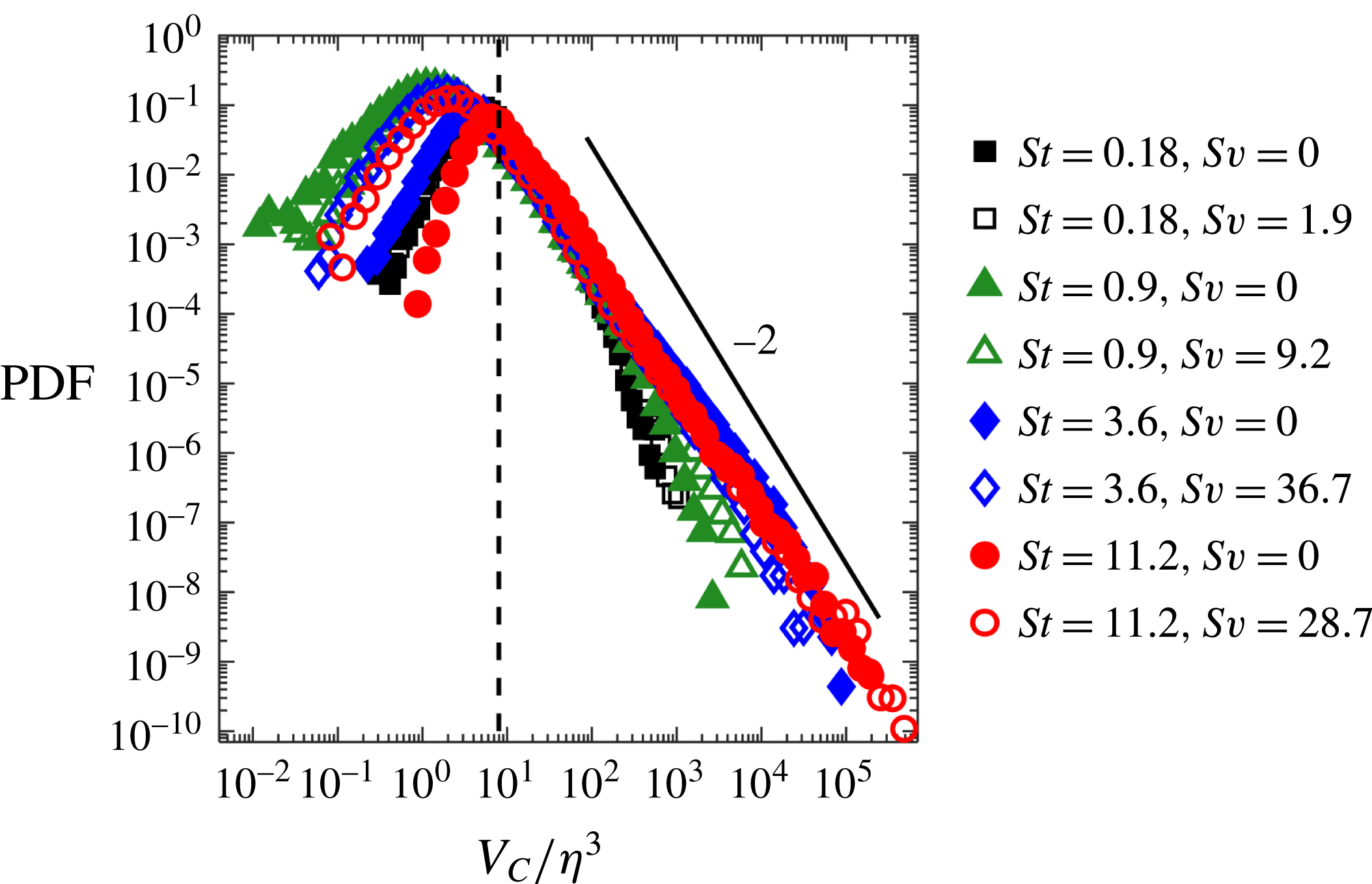
Similar considerations can be made observing the PDFs of cluster volumes (figure 3). For volumes larger than the
 $8\unicode[STIX]{x1D702}^{3}$
threshold, the distributions consistently follow a power law, indicating the clusters in this size range exhibit self-similarity. The latter is visible over more than four decades for the higher-St cases, which demonstrates how coherent clustering extends up to the integral scales, which for the present configuration corresponds to about
 $60\unicode[STIX]{x1D702}$
(Frankel et al.
Reference Frankel, Pouransari, Coletti and Mani2016). The slope is close to the value of
 $-2$
found experimentally by Monchaux et al. (Reference Monchaux, Bourgoin and Cartellier2010) and Obligado et al. (Reference Obligado, Teitelbaum, Cartellier, Mininni and Bourgoin2014) for the areas of clusters obtained by planar particle imaging. Moisy & Jiménez (Reference Moisy and Jiménez2004) found that turbulent structures also follow a
 $-2$
power-law behaviour, while Yoshimoto & Goto (Reference Yoshimoto and Goto2007) reported a
 $-1.8$
exponent for PDFs of void volumes separating particle clusters.
PDFs of cluster volume. The coherent cluster volume limit of
 $8\unicode[STIX]{x1D702}^{3}$
is marked with a vertical dashed line.

Besides being common to all investigated cases, the volume threshold appears reasonably robust to potential subsampling bias: removing as many as 95 % of the particles, the threshold moves from
 $(2\unicode[STIX]{x1D702})^{3}$
to at most
 $(5\unicode[STIX]{x1D702})^{3}$
(see figure 4). The difference is likely due to the fact that, with much fewer particles in the domain, small clusters are unlikely to exhibit self-similarity. For reference, the threshold
 $8\unicode[STIX]{x1D702}^{3}$
is between 1.2 and 1.5 times larger than
 $V^{\ast }$
, depending on the particle parameters.
Despite being seemingly robust, the value of the volume threshold should not be regarded as bearing a special physical significance. It might in fact depend on the turbulence Reynolds number, and would likely be affected by the physical mechanisms neglected in the present study (notably mass loading and particle finite size). Its value merely represents a size limit above which, in the present conditions, the clusters display self-similarity. We find it remarkable that this happens right at the dissipative scales of the turbulence. On one side, this suggests that these clusters are brought together by flow structures. On the other, it also implies that the coherent clusters, in the presence of significant two-way coupling, could have a relatively stronger effect on the fluid dynamics.
Cluster surface area versus the cubic root of cluster volume for the
 $St=3.6$
,
 $Sv=0$
case, subsampled at different fractions P of the total number of particles in the domain. Other St,
 $Sv$
cases display similar trends.

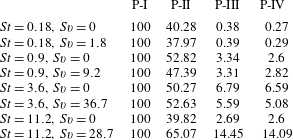
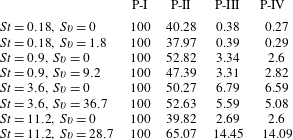
In order to appreciate the result of the cluster identification process, we distinguish between four categories of particles. We term P-I the set of all particles in the simulation domain. P-II denotes the subset of particles whose Voronoï cells have volumes
 $V<V^{\ast }$
. These are not necessarily clustered particles, since they do not necessarily belong to a connected set of cells. The subset of the particles in P-II which additionally belong to connected groups of Voronoï cells are denoted as P-III. These sets qualify as clusters in the strict topological sense, but they do not necessarily display self-similarity. Finally, P-IV is the subset of P-III particles belonging to coherent clusters, i.e. with volumes
 $V_{C}>8\unicode[STIX]{x1D702}^{3}$
. The breakdown for each subset, given as a percentage of the total number of particles, is reported in table 3. P-II particles account for about half of the total, and when gravity is not acting, the cases with Stokes number close to unity show the highest P-II percentage. This is consistent with the notion that preferential concentration is maximized for
 $St\approx 1$
. However, only a small fraction of the P-II particles belong to connected clusters. This fraction tends to increase with
 $St$
, reflecting the trend of more inertial particles forming larger clusters (as visible in figure 3). As a consequence, most clusters in the
 $St=3.6$
and
 $St=11.2$
cases are above the
 $8\unicode[STIX]{x1D702}^{3}$
size threshold, and indeed the P-III and P-IV sets almost coincide. For smaller Stokes numbers the differences are instead significant, with up to 30 % of P-III particles not belonging to coherent clusters. It is noteworthy that only a relatively small fraction of the particles belongs to coherent clusters. However, we remark that by far the strongest drop in particle fraction is between groups P-II and P-III; that is, the most stringent condition is the requirement of belonging to a connected group (i.e. a cluster). Such requirement was similarly applied in all previous studies that used Voronoï analysis to identify individual clusters (e.g. Monchaux et al.
Reference Monchaux, Bourgoin and Cartellier2010; Obligado et al.
Reference Obligado, Teitelbaum, Cartellier, Mininni and Bourgoin2014; Zamansky et al.
Reference Zamansky, Coletti, Massot and Mani2016; Sumbekova et al.
Reference Sumbekova, Cartellier, Aliseda and Bourgoin2017). The smallness of such a fraction raises the question of the dynamic relevance of clustered particles (coherent or not) relative to the non-clustered particles. However, this can only be resolved by accurate two-way coupled simulations, which are outside of the scope of the present study.
Percentage of particles in the domain belonging to each category P-I–P-IV.
4 Cluster properties
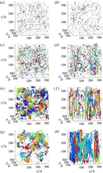
The coherent clusters are visualized in figure 5 by highlighting the Voronoï cells of each cluster in different colours. Many of the trends noted in previous studies are recovered – for example, the increase in size with increasing St (Yoshimoto & Goto Reference Yoshimoto and Goto2007) and the formation of vertically oriented streaks of particles with high
 $Sv$
(Woittiez, Jonker & Portela Reference Woittiez, Jonker and Portela2009). Some of the high-
 $Sv$
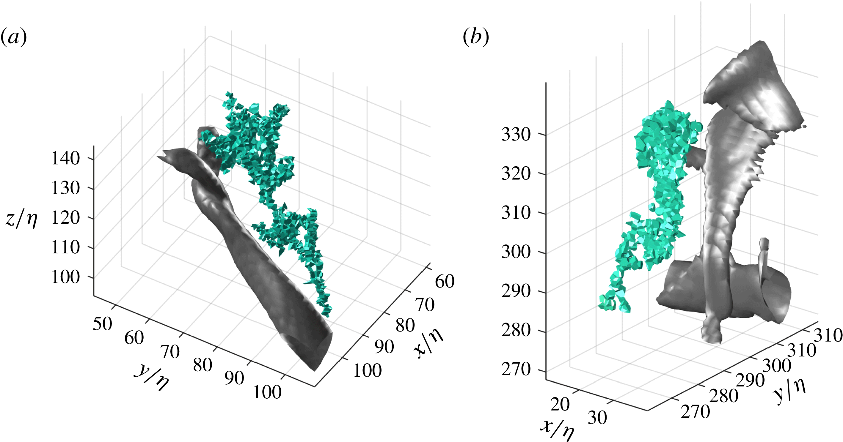
clusters seem to extend for the entire domain, but this is due to the colour coding (i.e. different clusters having the same colour and appearing as one). All considered cases verify the condition proposed by Ireland et al. (Reference Ireland, Bragg and Collins2016) for periodicity effects to be negligible. Figure 6 shows close-up views of two sample coherent clusters and nearby eddies in the
 $St=0.9$
,
 $Sv=0$
case and
 $St=3.6$
,
 $Sv=0$
case. The eddies are visualized with isosurfaces of enstrophy at a level of two standard deviations above the domain average. The clusters appear to stretch along the same direction and possess similar shapes as the eddy structures. In the present section we give quantitative expression to these qualitative observations.
Visualizations of coherent clusters for the eight considered cases: (a)
 $St=0.18$
,
 $Sv=0$
; (b)
 $St=0.18$
,
 $Sv=1.9$
; (c)
 $St=0.9$
,
 $Sv=0$
; (d)
 $St=0.9$
,
 $Sv=9.2$
; (e)
 $St=3.6$
,
 $Sv=0$
; (f)
 $St=3.6$
,
 $Sv=36.7$
; (g)
 $St=11.2$
,
 $Sv=0$
; (h)
 $St=11.2$
,
 $Sv=28.7$
. Colours are used to distinguish the individual clusters.

Sample coherent clusters and nearby eddies (identified by a level of enstrophy two standard deviations above the domain average) in the
 $St=0.9$
,
 $Sv=0$
case (a) and
 $St=3.6$
,
 $Sv=0$
case (b).

4.1 Cluster topology
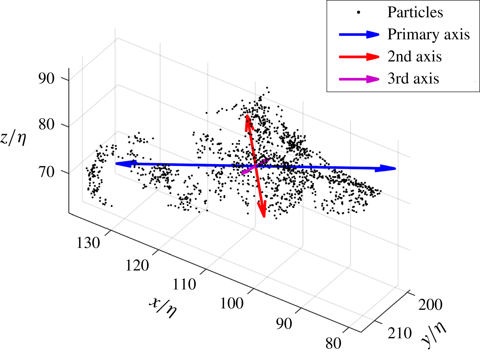
In order to characterize the general features of the particle distribution in each cluster, we use singular value decomposition (SVD) to find the principal axes and corresponding singular values for the particle set in each coherent cluster. SVD is a natural method to achieve a low-order description of a set of points in multi-dimensional spaces, the physical three-dimensional space being a clear example. By definition, the first principal axis of a set lies along the direction of the greatest spread of particle distances from the cluster centroid; the second principal axis lies along the direction of greatest spread within a plane normal to the first axis; the third principal axis is orthogonal to the first two and lies in the direction of minimum spread. The corresponding singular values are a measure of particle spread along each principal axis; specifically, a singular value normalized by the number of particles in the cluster gives the variance of the particle distances from the cluster centroid projected along that axis. An example of the principal axes of a coherent cluster is shown in figure 7, in which the length of each vector arrow is proportional to the corresponding singular value. The complex spatial distribution of the clustered particles is apparent.
Principal axes of a cluster found by singular value decomposition. The length of each vector arrow is proportional to the corresponding singular value.

The singular values
 $s_{1}\geqslant s_{2}\geqslant s_{3}$
are used here to define two aspect ratios for each cluster,
 $s_{2}/s_{1}$
and
 $s_{3}/s_{2}$
. These can be interpreted by considering the limiting (
 $s_{2}/s_{1}$
,
 $s_{3}/s_{2}$
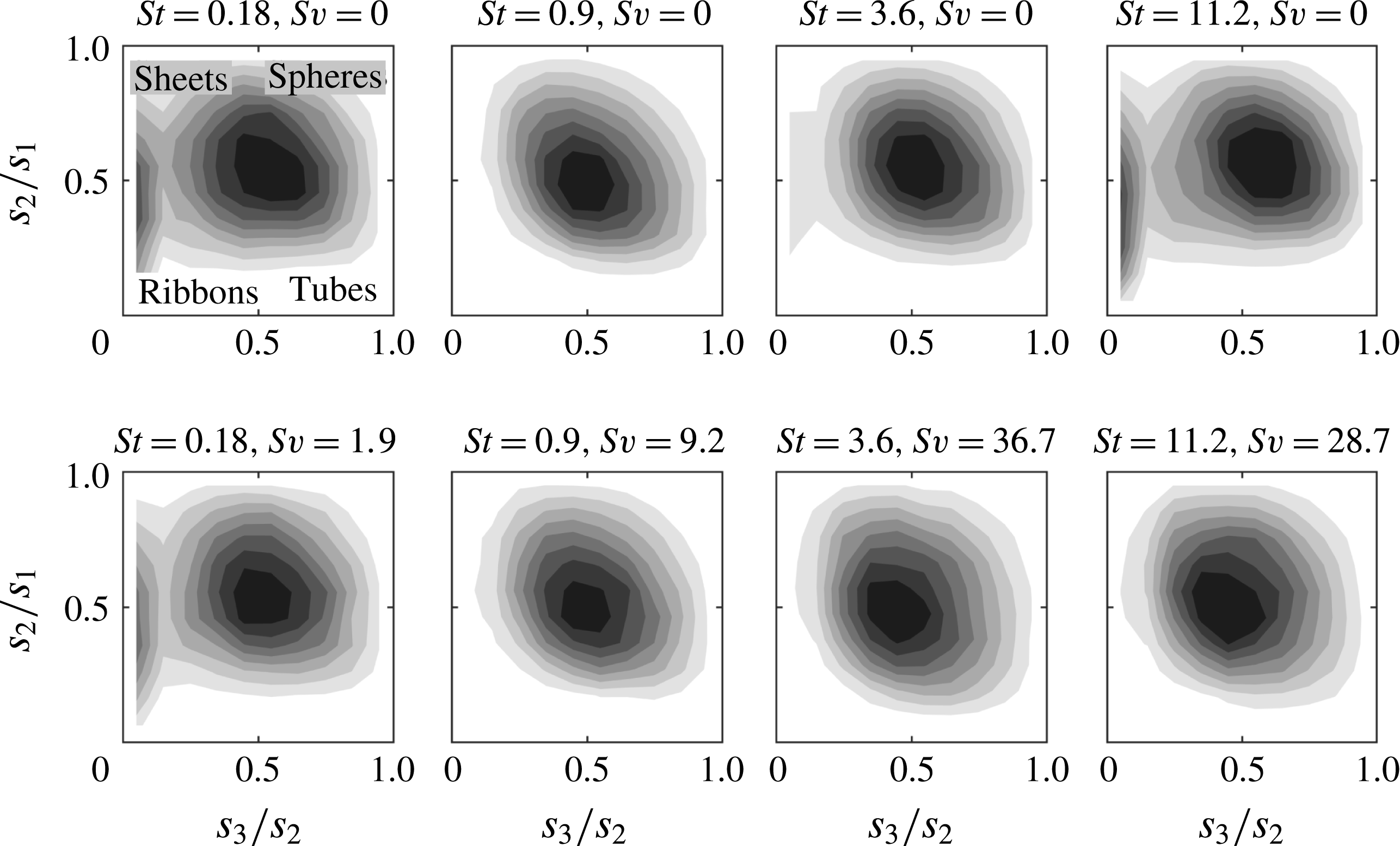
) cases: (0, 0) corresponds to a thin ribbon; (1, 0) corresponds to a thin sheet; (0, 1) corresponds to a thin rod; and (1, 1) corresponds to a sphere. The joint PDF of
 $s_{2}/s_{1}$
and
 $s_{3}/s_{2}$
is shown figure 8. For all considered cases the most likely combination of aspect ratios is about (0.5, 0.5), which corresponds to proportions 4 : 2 : 1. The cases with gravity exhibit somewhat lower aspect ratios, which reflects the tendency to form elongated streaks. The local maximum at very low values of
 $s_{3}/s_{2}$
present in some of the cases is due to small clusters with relatively low particle counts, which tend to be thin in one dimension.
Joint PDFs of aspect ratios
 $s_{2}/s_{1}$
and
 $s_{3}/s_{2}$
of the coherent clusters, based on singular value decomposition. Labels in the first panel indicate the topology in the extreme cases in which the aspect ratios are either 0 or 1.

This analysis is similar to the one carried out by Moisy & Jiménez (Reference Moisy and Jiménez2004) for turbulent flow structures characterized by high vorticity and high strain. However, these authors used a different set of length scales: for each structure of volume V they defined three lengths scales
 $r_{1}\leqslant r_{2}\leqslant r_{3}$
such that
 $V=r_{1}r_{2}r_{3}$
; the outer scale
 $r_{3}$
is the size of the smallest embedding box that fully contains the cluster, the inner scale
 $r_{1}$
is the size of the largest box that can be fully embedded in the cluster, and the intermediate scale
 $r_{2}$
is computed as
 $V/(r_{1}r_{3})$
. The set of aspect ratios
 $r_{1}/r_{2}$
and
 $r_{2}/r_{3}$
has the same geometrical interpretation as
 $s_{3}/s_{2}$
and
 $s_{2}/s_{1}$
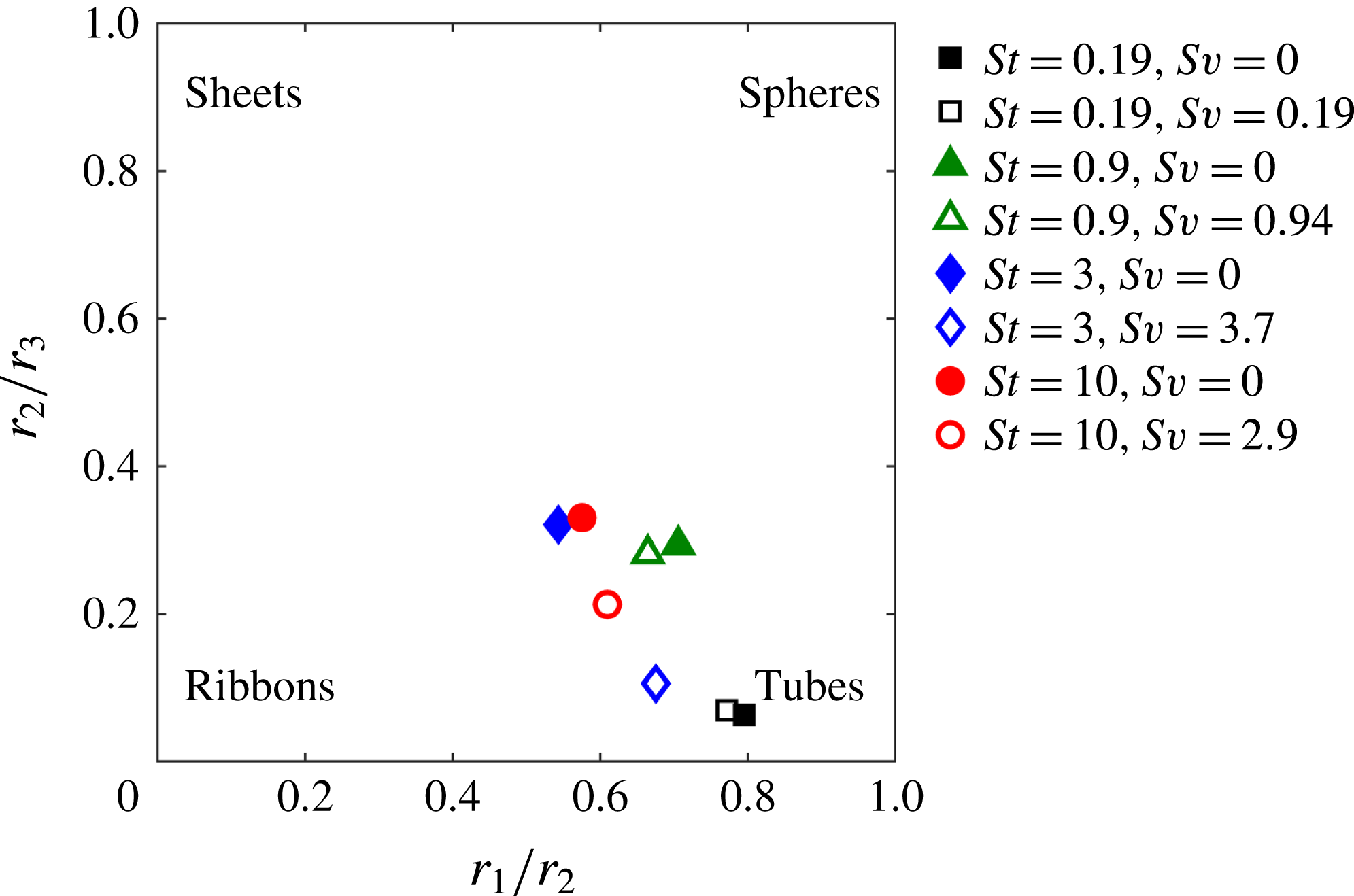
. We also applied this method, and the average values
 $\langle r_{1}/r_{2}\rangle$
and
 $\langle r_{2}/r_{3}\rangle$
are shown in figure 9. The inner scale
 $r_{1}$
is computed from a variation of the box-counting method, and is reliably obtained only for relatively large clusters. We therefore only consider clusters with
 $V_{C}>100\unicode[STIX]{x1D702}^{3}$
. There is not a large spread between cases, but compared to the SVD-based aspect ratios,
 $\langle r_{1}/r_{2}\rangle$
and
 $\langle r_{2}/r_{3}\rangle$
indicate more tubular and generally thinner shapes.
Mean aspect ratios
 $\langle r_{1}/r_{2}\rangle$
and
 $\langle r_{2}/r_{3}\rangle$
of coherent clusters with a volume larger than
 $100\unicode[STIX]{x1D702}^{3}$
, based on embedding and embedded boxes. The topologies are indicated in the extreme cases in which the aspect ratios are either 0 or 1.

We remark that the method of Moisy & Jiménez (Reference Moisy and Jiménez2004) does not take into account the interior structure of the particle distribution within the cluster: as the characteristic lengths are quantified by embedding and embedded boxes,
 $r_{3}$
and
 $r_{1}$
represent estimates of the ‘maximum length’ and ‘minimum waist’ of the clusters, respectively. The SVD method on the other hand uses the entire particle set in each cluster. While both methods provide useful indications of the clusters’ aspect ratio, neither of them can provide a full description of their shape, because the complex fractal structure of the particle distribution is not accounted for. This is discussed in § 4.3.
4.2 Particle concentration and distribution
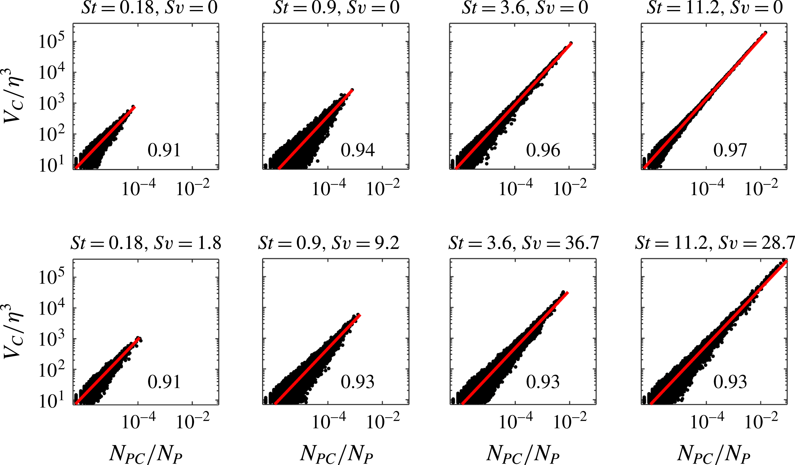
To determine how the particle concentration varies with cluster size, scatter plots of cluster volumes
 $V_{C}$
against particle counts
 $N_{PC}$
are displayed in figure 10. The concentration within a cluster is given by
 $C_{C}=N_{PC}/V_{C}$
, so the mean concentration is given by
 $$\begin{eqnarray}C_{C}=\frac{\text{d}V_{C}}{\text{d}N_{PC}}.\end{eqnarray}$$
The exponent of the fitting power law (red line in figure 10) is close to one, indicating that the volume and particle count of clusters are nearly linearly related, and therefore the mean concentration is approximately constant throughout the range of cluster sizes. We note that, for the small clusters, there is significant scatter around the linear trend. This is partly due to the fact that, when the number of particles in a cluster is relatively small, the calculated volume (which is in fact the volume of the set of its Voronoï cells) is a less accurate approximation of the cluster size. The value of the mean concentration for each St,
 $Sv$
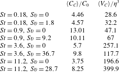
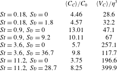
case is given in table 4 along with the mean volume of the coherent clusters. The concentration in the clusters is about one order of magnitude higher than the domain average, with the highest values found for St close to unity, as expected. For
 $St<1$
, gravitational settling somewhat reduces the in-cluster concentration (the change for
 $St=0.18$
being marginal); for
 $St>1$
, the opposite is true, and settling increases the in-cluster concentration. Such a trend was found in multiple recent studies (e.g. Bec, Homann & Ray Reference Bec, Homann and Ray2014; Gustavsson, Vajedi & Mehlig Reference Gustavsson, Vajedi and Mehlig2014; Ireland et al.
Reference Ireland, Bragg and Collins2016; Matsuda, Onishi & Takahashi Reference Matsuda, Onishi and Takahashi2017). The consensus is that strongly inertial and fast-falling particles become uncorrelated from the turbulent flow structures, but the mechanism for enhanced clustering in these condition is still debated. The mean cluster volume generally increases with St and
 $Sv$
, confirming the trend visible in figures 3 and 5. Finding larger clusters at higher St is expected, because more inertial particles respond to larger eddies (Goto & Vassilicos Reference Goto and Vassilicos2006; Yoshimoto & Goto Reference Yoshimoto and Goto2007). On the other hand, the trend with
 $Sv$
suggests the presence of a clustering mechanism other than the classic centrifugal effect, such as the sweep-stick mechanism (Goto & Vassilicos Reference Goto and Vassilicos2008) and/or the path-history effect (Bragg & Collins Reference Bragg and Collins2014), as we discuss in § 5.
Cluster volume normalized by the Kolmogorov length scale versus cluster particle counts normalized by the total number of particles in the domain.

Mean particle concentration within clusters normalized by the global concentration, and mean cluster volume normalized by the Kolmogorov length scale.
To characterize the nature and spatial extent of particle clustering, we can use the radial distribution function (RDF):
 $$\begin{eqnarray}g(r_{i})=\frac{P_{i}/v_{i}}{P/v},\end{eqnarray}$$
where
 $P_{i}$
is the number of pairs of particles separated by a distance
 $r_{i}\pm \unicode[STIX]{x0394}r/2$
,
 $v_{i}=4\unicode[STIX]{x03C0}[(r_{i}+\unicode[STIX]{x0394}r/2)^{3}-(r_{i}-\unicode[STIX]{x0394}r/2)^{3}]/3$
is the volume of the spherical shell of mean radius
 $r_{i}$
, and
 $P=N_{P}(N_{P}-1)/2$
is the total number of particle pairs in the simulation domain
 $v$
. In order to study anisotropic effects due to gravity, the angular distribution function (ADF, Gualtieri et al.
Reference Gualtieri, Picano and Casciola2009) can be derived by binning the particle pairs using both the distance and the angle spanned by the inter-particle separation vector and the vertical:
 $$\begin{eqnarray}g(r_{i},\unicode[STIX]{x1D703}_{j})=\frac{P_{i,j}/v_{i,j}}{P/v}.\end{eqnarray}$$
Here
 $P_{i,j}$
is the number of particle pairs separated by distance
 $r_{i}\pm \unicode[STIX]{x0394}r/2$
and whose displacement vector has an orientation
 $\unicode[STIX]{x1D703}_{j}\pm \unicode[STIX]{x0394}\unicode[STIX]{x1D703}/2$
relative to the vertical, and
 $v_{i,j}$
is the volume of the part of the
 $i$
th spherical shell contained in the
 $j$
th angular bin. A power-law behaviour
 $g(r)\propto r^{-\unicode[STIX]{x1D6FC}}$
of the RDF or ADF indicates self-similar clustering. The value of
 $\unicode[STIX]{x1D6FC}$
is used to find the correlation dimension
 $D_{2}=3-\unicode[STIX]{x1D6FC}$
, which characterizes the clustering behaviour of a particle distribution (see for example Fessler, Kulick & Eaton Reference Fessler, Kulick and Eaton1994; Bec et al.
Reference Bec, Biferale, Cencini, Lanotte, Musacchio and Toschi2007; Gualtieri et al.
Reference Gualtieri, Picano and Casciola2009). A steeper slope (i.e. a lower value of
 $D_{2}$
) implies a higher degree of local accumulation.
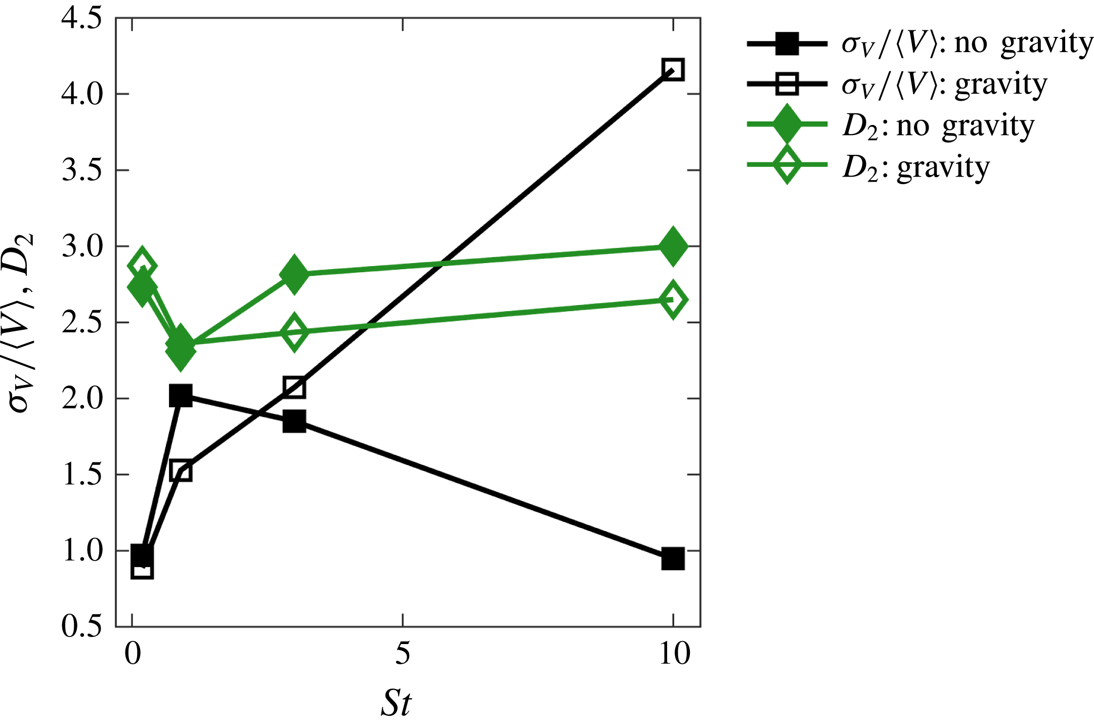
We first consider the RDF for the full set of P-I particles. Figure 11 presents the dependence of
 $D_{2}$
(calculated from a power-law fit over the range
 $0.2<r/\unicode[STIX]{x1D702}<1.5$
) with Stokes number. The normalized standard deviation of the PDF of Voronoï cell size
 $\unicode[STIX]{x1D70E}_{V}/\langle V\rangle$
is also plotted. For the cases without gravity,
 $D_{2}$
shows a minimum and
 $\unicode[STIX]{x1D70E}_{V}/\langle V\rangle$
a maximum around
 $St\approx 1$
. This is expected, as both quantities are regarded as measures of clustering (Bec et al.
Reference Bec, Biferale, Cencini, Lanotte, Musacchio and Toschi2007; Monchaux et al.
Reference Monchaux, Bourgoin and Cartellier2010). For the cases with gravitational settling,
 $D_{2}$
has a similar (although less pronounced) behaviour, while
 $\unicode[STIX]{x1D70E}_{V}/\langle V\rangle$
increases with St. This suggests that the standard deviation of the Voronoï volumes PDF should be interpreted with caution. In fact, besides the local concentration in the clusters, the latter is also a function of the size of the voids, which in turn depends in a non-trivial way on the number and spatial distribution of the clusters.
Normalized standard deviation of the Voronoï cell size
 $\unicode[STIX]{x1D70E}_{V}/\langle V\rangle$
and correlation dimension
 $D_{2}$
for the full set of P-I particles versus Stokes number.

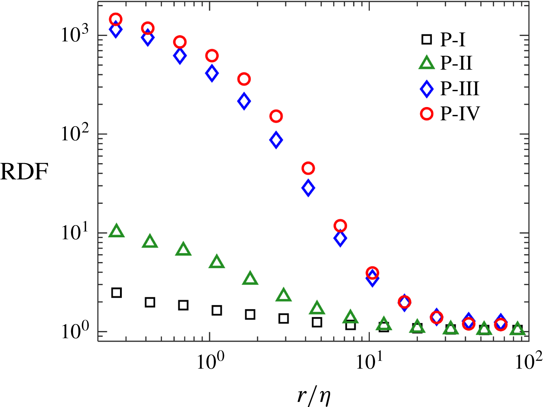
To assess the effect of the cluster identification process, in figure 12 the RDFs of the four particle categories P-I through P-IV are shown for the
 $St=0.18$
,
 $Sv=0$
case. The values of
 $D_{2}$
follow a generally decreasing trend from P-I (
 $D_{2}=2.73$
) to P-IV (
 $D_{2}=2.38$
), reflecting the higher degree of spatial organization and accumulation of the clustered particles. The trend is the same for all St,
 $Sv$
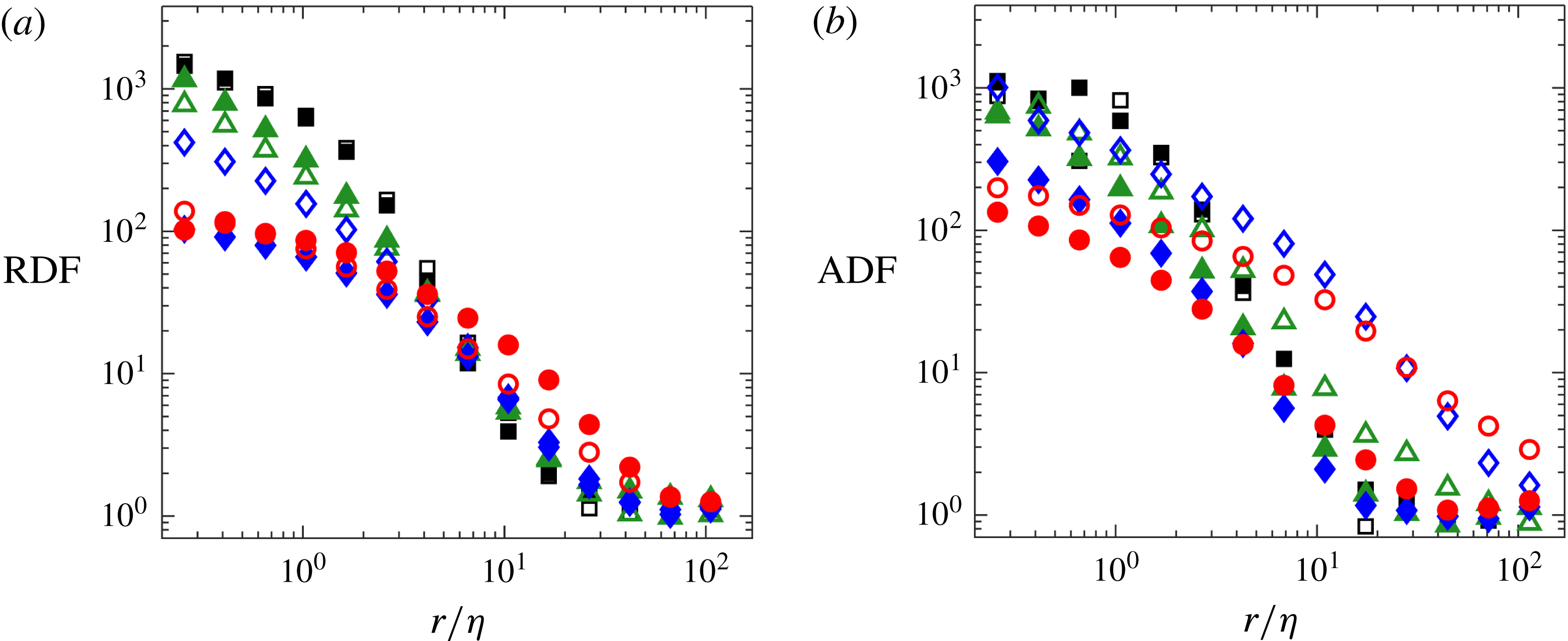
cases. Focusing on the coherent clusters, figure 13(a) shows RDFs of the P-IV particle distributions. As expected, the steepest slope is found for St near unity, corresponding to a minimum value of
 $D_{2}$
, both in the cases with and without gravity. The range over which the RDF remains greater than one indicates the length scale over which the clustering occurs. This increases monotonically with St, consistently with the above-mentioned tendency of more inertial particles to form larger clusters. To highlight the spatial organization of the clusters in the presence of gravity, figure 13(b) displays the ADF calculated for the
 $Sv>0$
cases for angular bins
 $|\unicode[STIX]{x1D703}|=[0^{\circ },10^{\circ }]$
(vertical direction) and
 $|\unicode[STIX]{x1D703}|=[80^{\circ },100^{\circ }]$
(horizontal direction). For the high-St, high-
 $Sv$
cases, the vertical ADF decays over much larger distances than the horizontal ADF, a signature of the vertical particle streaks, which can have lengths greater than
 $100\unicode[STIX]{x1D702}$
(figure 5).
RDFs of the four particle categories P-I–P-IV for the
 $St=0.18$
,
 $Sv=0$
case.

(a) RDFs of the P-IV particle distributions for all cases, with filled symbols for cases without gravity and empty symbols for cases with gravity. (b) ADFs calculated for the
 $Sv>0$
cases for angular bins
 $|\unicode[STIX]{x1D703}|=[0^{\circ },10^{\circ }]$
(vertical direction, empty symbols) and
 $|\unicode[STIX]{x1D703}|=[80^{\circ },100^{\circ }]$
(horizontal direction, filled symbols). In both plots, the cases are as follows:
 $St=0.18$
(black squares),
 $St=0.9$
(green triangles),
 $St=3.6$
(blue diamonds), and
 $St=11.2$
(red circles).

Taken together, these results demonstrate how, besides exhibiting a power-law decay of their size distribution (which indicates statistical self-similarity among the various objects), the individual coherent clusters also display geometrically self-similar structures. Their fractal nature is also reflected in the highly convoluted boundaries, which may have important implications for, for example, the mixing between laden and unladen fluid. The general shape of the clusters (tubular rather than planar) also appears to depend on the object size. Overall, the results suggest a link between the geometry of the coherent clusters and that of the underlying turbulent motions. To corroborate these observations, it will be of interest to use larger simulations and evaluate the effect of the turbulence Reynolds number (and therefore of the range of scales) on the quantities calculated here.
4.3 Fractal dimensions of individual clusters
Being self-similar objects, the coherent clusters display a complex topology which can be described in a compact manner by their fractal dimension. As discussed below, different aspects of their features (global shape, small-scale structure, enveloping surface) can be described via different fractal dimension definitions; here we use some of the more common, often employed to characterize physical and biological systems (Falconer Reference Falconer2004). This quantitative characterization may also help in the development of low-order models of the cluster features and behaviour. The fractal structure of inertial particles fields in turbulence has been the subject of previous investigations (e.g. Bec Reference Bec2003; Bec et al. Reference Bec, Biferale, Cencini, Lanotte, Musacchio and Toschi2007; Calzavarini et al. Reference Calzavarini, Kerscher, Lohse and Toschi2008). Here we instead focus on the fractal dimension of individual clusters. The relation between the fractal description of individual structures and that of the global field in the domain is not straightforward, see Moisy & Jiménez (Reference Moisy and Jiménez2004).
Several definitions of fractal dimension are commonly used, and are in general not equivalent except for mathematically constructed fractal sets. Moreover, inertial particles in turbulence have been shown to resemble multifractal sets (Bec Reference Bec2005), i.e. to possess different fractal properties at different scales. Multifractal sets are characterized by a range of fractal dimensions, among which are the well-known box-counting dimension
 $D_{0}$
and correlation dimension
 $D_{2}$
(Grassberger & Procaccia Reference Grassberger and Procaccia1983). Here we calculate both dimensions for the sets of particles belonging to individual clusters, as well as the fractal dimension of the cluster surface (defined in the sense specified in § 3). Only the number
 $N_{C}^{\prime }$
of clusters larger than
 $100\unicode[STIX]{x1D702}^{3}$
are analysed; smaller clusters did not have sufficient separation of scales to obtain good fractal dimension estimates. Depending on the case,
 $N_{C}^{\prime }$
ranges from several hundred to more than one thousand.
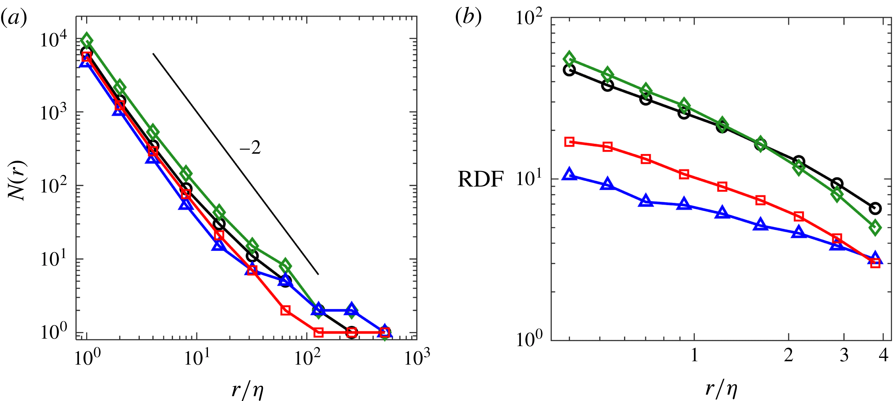
To determine the cluster box-counting dimension
 $D_{0C}$
, the portion of the domain containing each cluster is divided into non-overlapping cubes of side length r, and the number of boxes
 $N(r)$
containing at least one particle belonging to the cluster is counted. For large enough clusters, the number of boxes N needed to contain the full particle set follows a power law
 $N\propto r^{-D_{0}}$
over some range of r. As an example, plots of
 $N(r)$
for the four largest clusters of the
 $St=0.9$
,
 $Sv=0$
case are shown in figure 14(a). A fit through the power-law region in the range
 $1<r/\unicode[STIX]{x1D702}<8$
is used to calculate
 $D_{0C}$
for each cluster. To determine the correlation dimension of individual clusters
 $D_{2C}$
(not to be confused with
 $D_{2}$
, calculated over the entire particle set), the RDF of the particles in each cluster is considered and a best fit is applied to the power-law region in the range
 $0.5<r/\unicode[STIX]{x1D702}<1.5$
. Figure 14(b) shows RDFs for the same four clusters as in figure 14(a). Finally, the surface area dimension
 $D_{S}$
is found by fitting a power law to the scatter plots of cluster surface area against cluster volume (see figure 4).
(a) Number of boxes versus box size normalized by the Kolmogorov length for the four largest clusters of the
 $St=0.9$
,
 $Sv=0$
case. The box-counting dimensions were found by fitting power laws in the range
 $1<r/\unicode[STIX]{x1D702}<8$
. (b) RDFs for the same four clusters. The correlation dimensions were found by fitting power laws in the range
 $0.5<r/\unicode[STIX]{x1D702}<1.5$
.

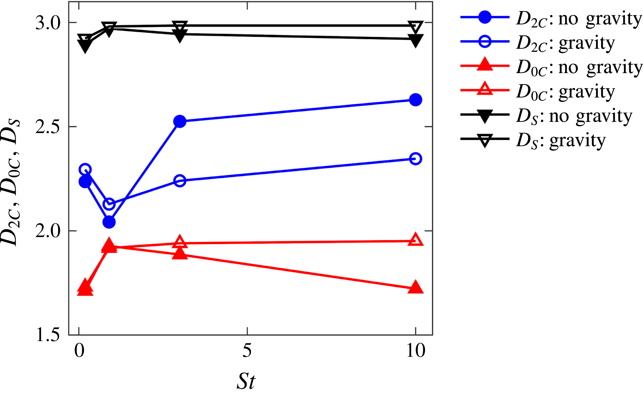
 $D_{0C}$
,
 $D_{2C}$
, and
 $D_{S}$
as a function of Stokes number, calculated as the average over the
 $N_{C}^{\prime }$
coherent clusters with volumes larger than
 $100\unicode[STIX]{x1D702}^{3}$
.

Figure 15 shows the values of
 $D_{0C}$
,
 $D_{2C}$
, and
 $D_{S}$
as a function of St, calculated as the average over the
 $N_{C}^{\prime }$
coherent clusters for each case.
 $D_{2C}$
has a similar trend to
 $D_{2}$
(see figure 11), but the values are lower due to the higher degree of spatial organization. Macroscopically, both the correlation dimension and the box-counting dimension are measures of the dimensionality of the particle distributions: values near 1 correspond to clusters resembling rod-like objects, values near 2 correspond to sheet-like objects, and values near 3 correspond to globular objects. However, both dimensions characterize different geometrical aspects of the small-scale distribution. In particular,
 $D_{2C}$
gives more weight to regions with high particle number densities (Gustavsson & Mehlig Reference Gustavsson and Mehlig2016). The difference between the two is thus not unexpected. Still, assuming the particles in each cluster follow the multifractal formalism, one would expect
 $D_{2C}\leqslant D_{0C}$
(Grassberger & Procaccia Reference Grassberger and Procaccia1983), in contrast to what is found here. However, one should consider that, as we are well outside of the limit
 $St\ll 1$
, the clusters may not exactly follow a multifractal behaviour. Moreover, we note that large uncertainties are likely associated to
 $D_{0C}$
, which is known to be very sensitive to discreteness effects and other sources of error that can significantly limit its robustness (Falconer Reference Falconer2004). Nevertheless, it is remarkable that the present values of
 $D_{0C}$
are close to the value of 1.7 obtained by Moisy & Jiménez (Reference Moisy and Jiménez2004) for individual high-shear structures in homogeneous isotropic turbulence.
 $D_{S}$
characterizes the surface of the clusters rather than their particle distribution, and is bounded by
 $2\leqslant D_{S}\leqslant 3$
. The limit
 $D_{S}=2$
is recovered for clusters enveloped by perfectly smooth surfaces, and the dimension increases as the cluster surface becomes more convoluted and therefore more space-filling.
 $D_{S}$
is found to be 2.85 or larger for all cases, confirming the visual impression that the borders of the clusters are extremely convoluted (see figure 6). As shown in figure 4, the values of
 $D_{S}$
are robust to possible subsampling bias.
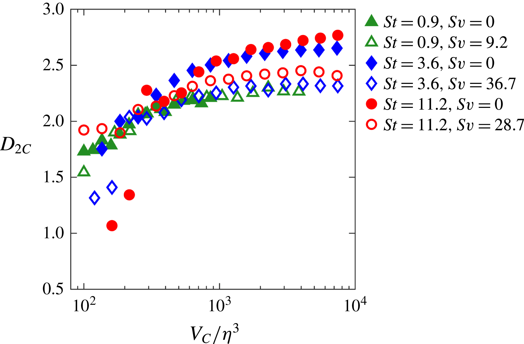
Correlation dimension of the coherent clusters conditionally averaged on their volume, for clusters with volumes larger than
 $100\unicode[STIX]{x1D702}^{3}$
. The
 $St=0.18$
cases are not shown because the number of large clusters for each data point is not sufficient for a statistically robust estimate.

Given that coherent clusters exist over a wide range of scales, it is of interest to investigate whether their fractal dimension changes with their size. Figure 16 shows
 $D_{2C}$
conditionally averaged on
 $V_{C}$
. The
 $St=0.18$
cases are not shown because the number of clusters for each data point is not sufficient for a statistically robust estimate. It is observed that the correlation dimension markedly increases with the cluster volume, and seems to plateau at values dependent on St and
 $Sv$
(although the limited range of scales cannot rule out further increase at larger volumes). For the cases with
 $St=O(1)$
,
 $D_{2C}$
for the large clusters tends to values close to the 2.6 value found by Calzavarini et al. (Reference Calzavarini, Kerscher, Lohse and Toschi2008) for the Kaplan–Yorke dimension in similar regimes. The dependence of
 $D_{2C}$
with the cluster size suggests that smaller clusters tend to be more tubular, and larger clusters tend to be more planar or globular. Under the assumption that clusters are a reflection of the eddy structures contributing to their formation, this trend appears consistent with the picture emerging from recent investigations of the geometry of eddy structures in homogeneous isotropic turbulence. In particular, Bermejo-Moreno, Pullin & Horiuti (Reference Bermejo-Moreno, Pullin and Horiuti2009) analysed isosurfaces of the curvelet transform of enstrophy and dissipation fields, and showed a transition from tubular to blob-like shapes with increasing scale. A similar conclusion was reached by Leung, Swaminathan & Davidson (Reference Leung, Swaminathan and Davidson2012) using a band-pass filtering approach at various scales. One should, however, be cautious when describing the topology, especially of large clusters, using
 $D_{2C}$
, as the latter is based on inter-particle correlation at small distances. Given the complex and multi-scale nature of the clusters, the use of multiple geometrical descriptors seems necessary to achieve a complete picture.
4.4 Preferential concentration
To examine the preferential concentration of clustered particles, the local concentration is conditionally averaged on the scalar vorticity magnitude
 $\unicode[STIX]{x1D6FA}$
and the strain rate
 $S$
for P-I and P-IV particles. Here
 $\unicode[STIX]{x1D6FA}=\unicode[STIX]{x1D6FA}_{ij}\unicode[STIX]{x1D6FA}_{ij}^{1/2}$
and
 $S=S_{ij}S_{ij}^{1/2}$
, where
 $\unicode[STIX]{x1D6FA}$
and
 $S$
are the rotation and strain-rate tensors, respectively. Following Wang & Maxey (Reference Wang and Maxey1993), we count the number of particles in each computational cell (centred at each grid point) in the domain, and bin those based on the local values of
 $\unicode[STIX]{x1D6FA}$
and
 $S$
. The concentration is then calculated as the number of particles counted for each bin, divided by the sum of the cell volumes associated to that bin. The conditionally averaged concentration is finally normalized by the global particle concentration of P-I and P-IV particles as appropriate, while
 $\unicode[STIX]{x1D6FA}$
and
 $S$
are normalized by their r.m.s. values. Results are shown in figure 17.
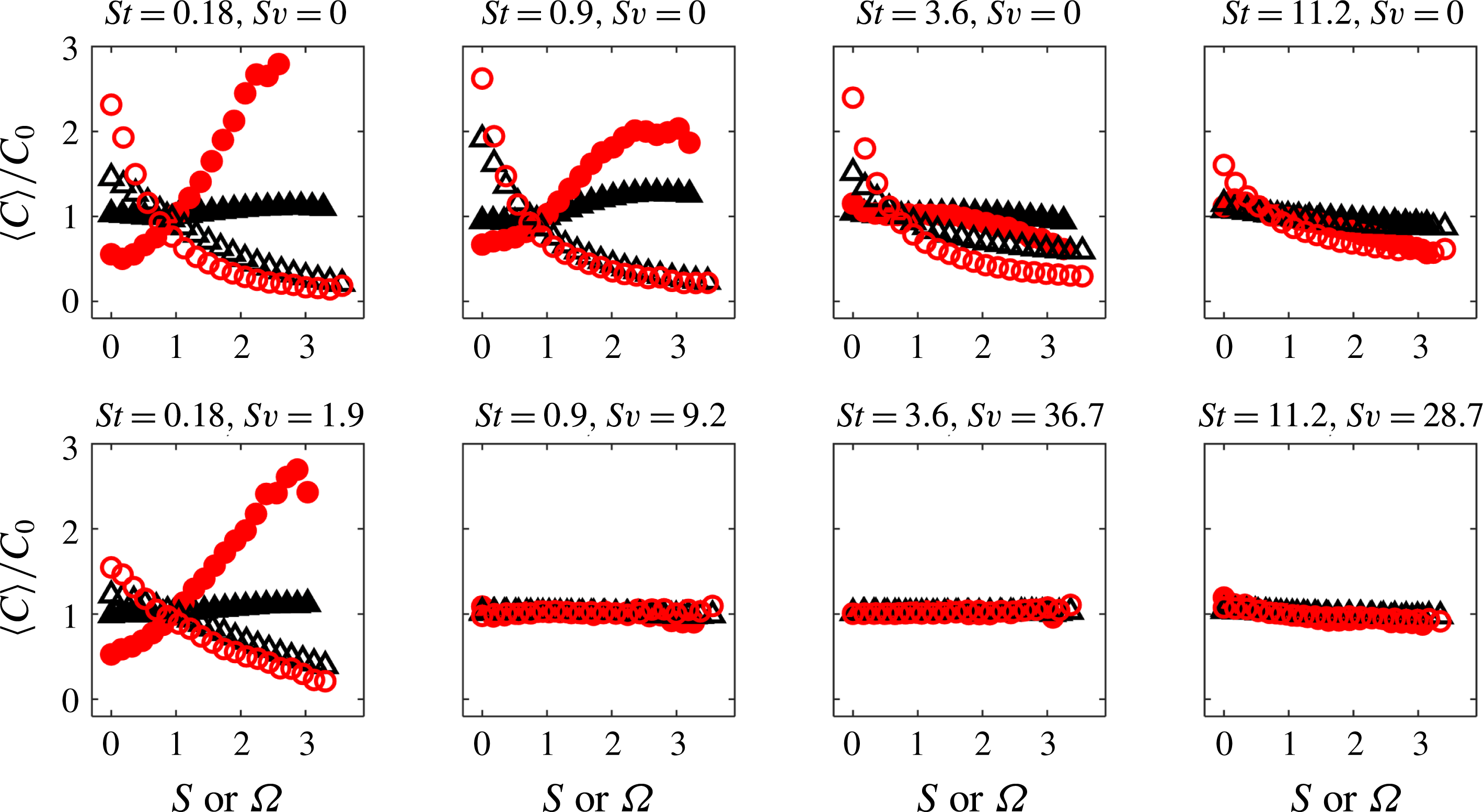
Local concentration conditionally averaged on the scalar vorticity magnitude
 $\unicode[STIX]{x1D6FA}$
(empty symbols) and the strain rate
 $S$
(filled symbols) for P-I (black triangles) and P-IV (red circles) particles. Local concentration is normalized by the global concentration, and
 $\unicode[STIX]{x1D6FA}$
and
 $S$
are normalized by their r.m.s. values.

For the
 $St=0.18$
and
 $St=0.9$
cases without gravitational effects, both P-I and P-IV particles are concentrated in areas of high strain and low vorticity. This is also true for the
 $St=0.18$
,
 $Sv=1.9$
case. Such effects (particularly the preferential sampling of high-strain regions) are highly intensified for particles in coherent clusters as compared to generic inertial particles. This is consistent with the classic picture of clusters being formed by preferential concentration of particles in high-strain, low-vorticity regions of the flow (e.g. Eaton & Fessler Reference Eaton and Fessler1994). At higher St, in the absence of gravity there is still a tendency for the particles to accumulate in low-vorticity regions, but no preference for high strain. Finally, for high-St settling particles there is no relation between local concentration and the local vorticity or strain: their large fall speed makes them uncorrelated from small-scale flow structures.
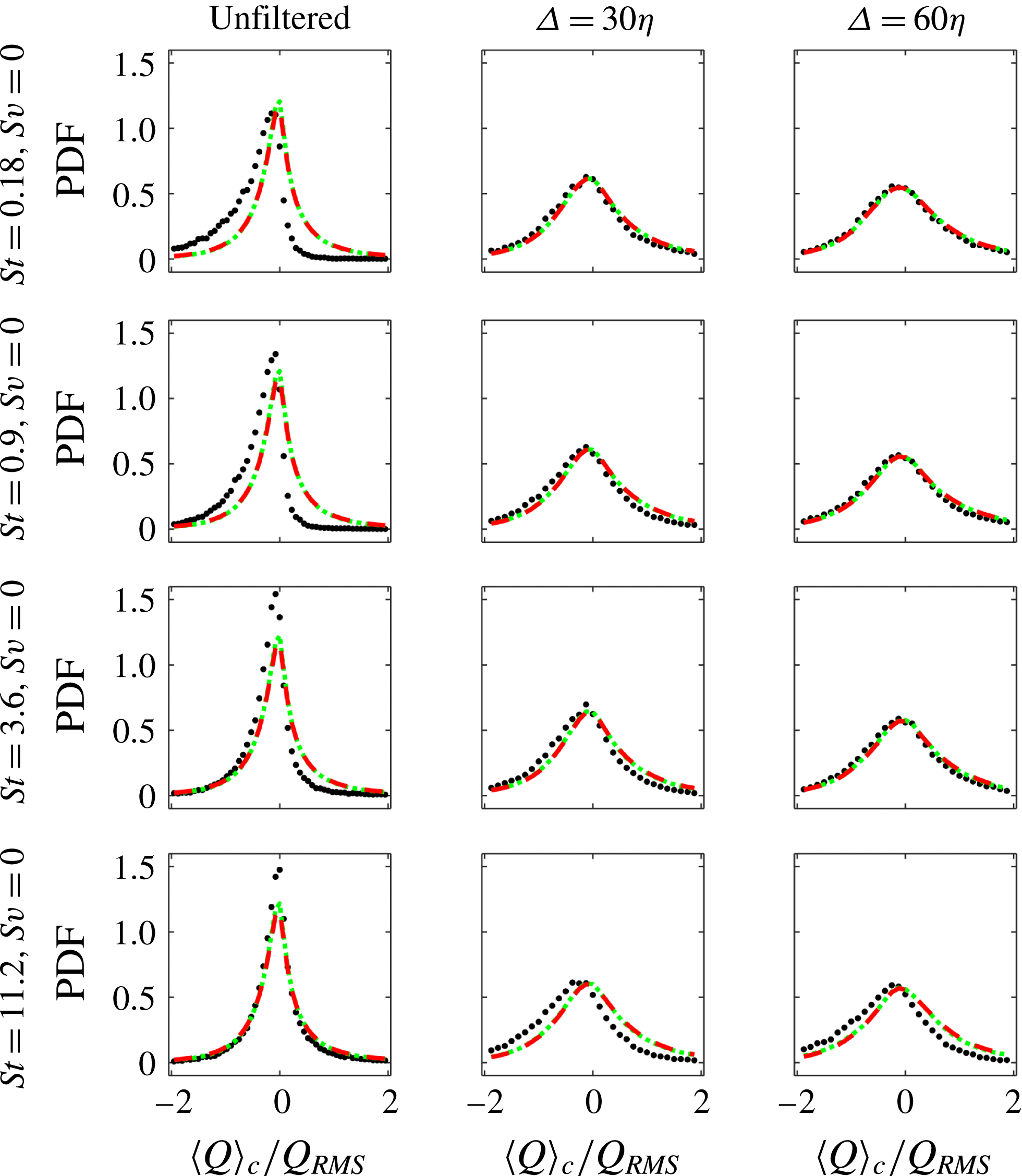
PDFs of
 $\langle Q\rangle _{C}$
(black dots) for the cases without gravity using unfiltered and filtered velocity fields. PDFs of
 $Q$
sampled at all P-I particle locations (red dashed line) and in the entire domain (green dotted line) are also shown for comparison. Values of
 $Q$
are normalized by their r.m.s. values.

The high-St particles are expected to be affected by large-scale flow structures (Yoshimoto & Goto Reference Yoshimoto and Goto2007), at least for zero or moderate settling. Preferential concentration is therefore examined for the particles in coherent clusters using a low-pass-filtered velocity field. The velocity field is filtered using a Gaussian kernel at two different length scales,
 $\unicode[STIX]{x1D6E5}=30\unicode[STIX]{x1D702}\approx L/2$
and
 $\unicode[STIX]{x1D6E5}=60\unicode[STIX]{x1D702}\approx L$
. Then the second invariant of the velocity gradient tensor,
 $Q=-1/2\;\text{tr}(\unicode[STIX]{x1D64E}^{2}-\unicode[STIX]{x1D734}^{2})$
, which is a measure of excess of vorticity over strain (Hunt, Wray & Moin Reference Hunt, Wray and Moin1988), is computed at each grid point in the flow field. A cluster-averaged value
 $\langle Q\rangle _{C}$
is obtained for each coherent cluster by averaging
 $Q$
over the grid points contained within the volume of that cluster. The PDF of
 $\langle Q\rangle _{C}$
is shown for the cases without gravity in figure 18 for unfiltered and filtered velocity fields. The PDFs of
 $Q$
sampled at all P-I particle locations and in the entire domain are also shown for comparison. All PDFs are normalized by
 $Q_{RMS}$
obtained from the flow field filtered with the corresponding kernel. In all cases, the PDF of
 $Q$
sampled at all particle locations is nearly identical to the PDF of
 $Q$
at all fluid grid points. In contrast, the PDF of
 $\langle Q\rangle _{C}$
shows that particles in coherent clusters oversample low-
 $Q$
regions, where strain is high compared to rotation. For the
 $St=0.18$
and
 $St=0.9$
cases this effect can be most clearly seen in the PDFs for the unfiltered velocity fields. For the
 $St=3.6$
and
 $St=11.2$
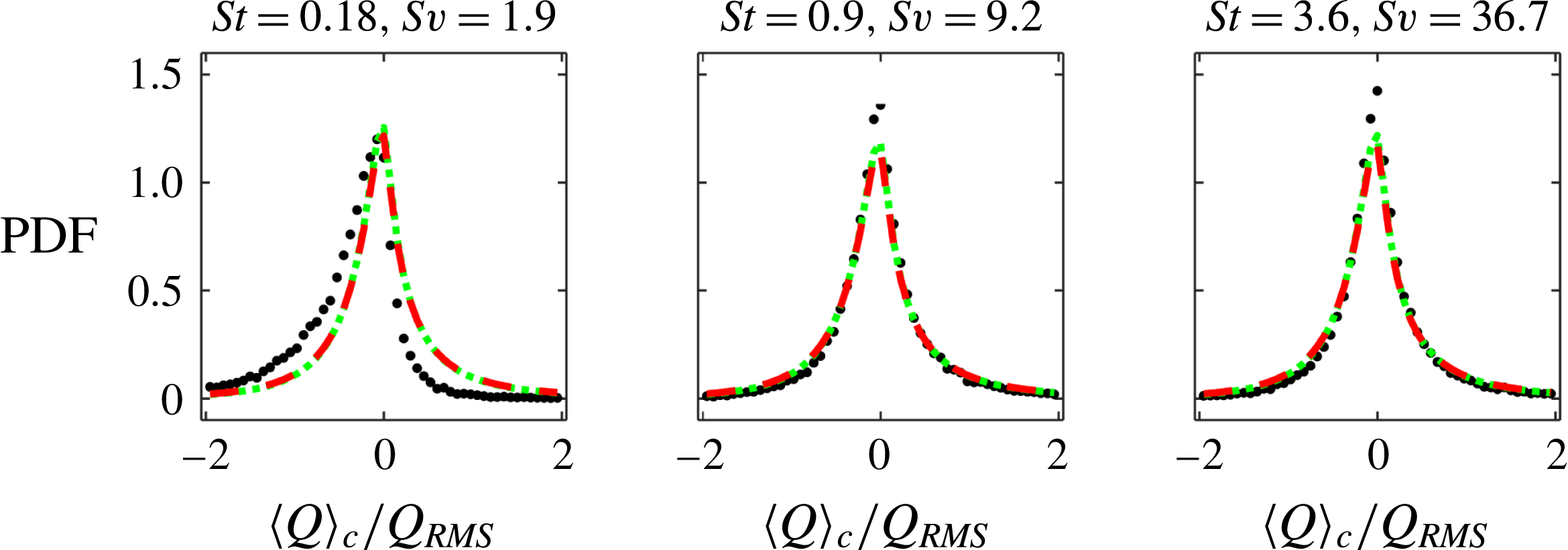
cases, the effect is visible in the PDFs of the velocity fields filtered at increasing scales, confirming the argument that particles cluster over scale with which they ‘resonate’ based on their response time (see, e.g., Yoshimoto & Goto Reference Yoshimoto and Goto2007). Figure 19 shows similar plots for the
 $St=0.18$
,
 $St=0.9$
, and
 $St=3.6$
cases with gravity, using unfiltered velocity fields. These confirm that, when
 $Sv\gtrsim 10$
, the clusters are uncorrelated from low-
 $Q$
regions due to the high settling velocity. This is true even considering the low-pass-filtered velocity fields at
 $\unicode[STIX]{x1D6E5}=30\unicode[STIX]{x1D702}$
and
 $\unicode[STIX]{x1D6E5}=60\unicode[STIX]{x1D702}$
(not shown).
PDFs of
 $\langle Q\rangle _{C}$
(black dots) for the
 $St=0.18$
,
 $St=0.9$
, and
 $St=3.6$
cases with gravity using unfiltered velocity fields. PDFs of
 $Q$
sampled at all P-I particle locations (red dashed line) and in the entire domain (green dotted line) are also shown for comparison. Values of
 $Q$
are normalized by their r.m.s. values.

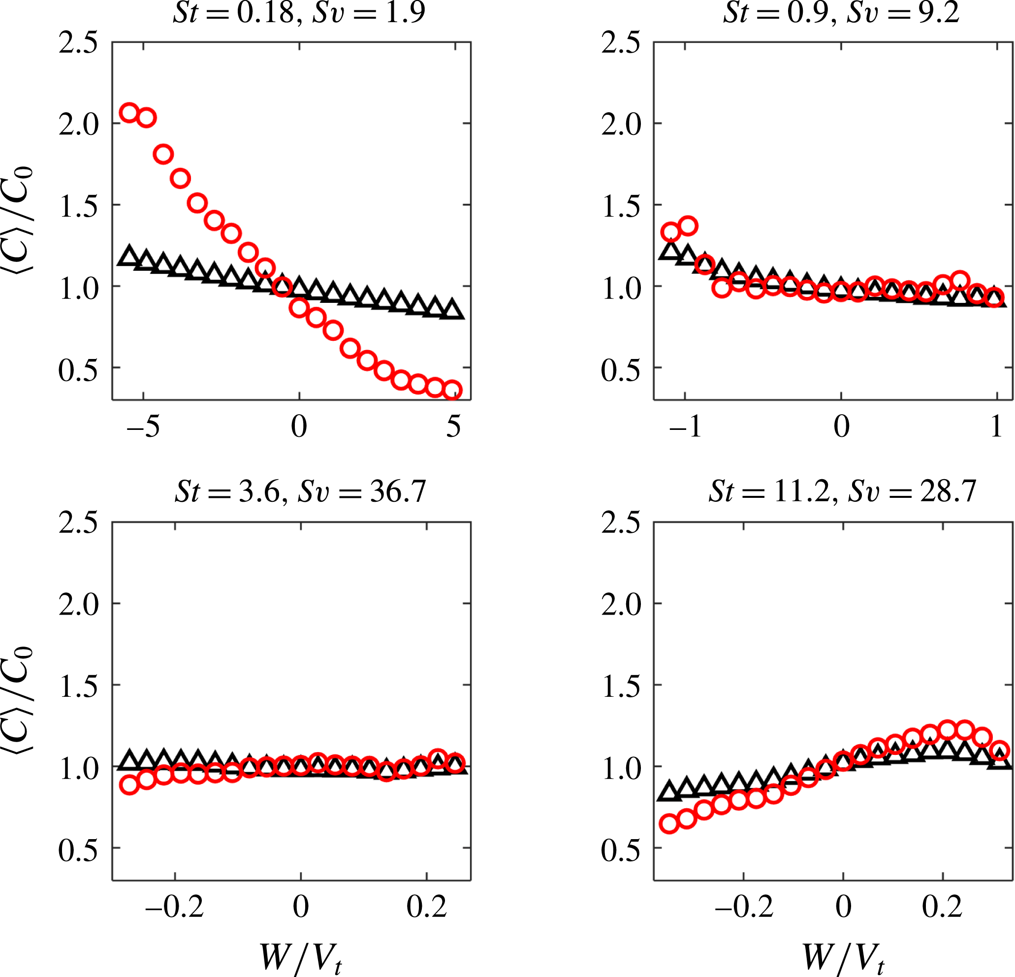
Local concentration for P-I (black triangles) and P-IV particles (red circles), conditionally averaged on the vertical fluid velocity for the cases with gravity. The local concentration is normalized by the global concentration, and velocities are normalized by the theoretical terminal velocity.

4.5 Particle settling
To investigate the effect of turbulence on the settling of the particles in the coherent clusters, in figure 20 the local concentration is conditionally averaged on the vertical fluid velocity W (taken positive when directed upward), with the same method used for
 $\unicode[STIX]{x1D6FA}$
and
 $S$
. Velocities are normalized by the still-fluid terminal velocity
 $V_{t}$
, and both P-I and P-IV particles are considered for comparison. Preferential sweeping, i.e. the tendency of the particles to favour downward regions of the flow (Wang & Maxey Reference Wang and Maxey1993), is apparent for the
 $St=0.18$
,
 $Sv=1.9$
case and, to a lesser extent, the
 $St=0.9$
,
 $Sv=9.2$
case. In the former case, P-IV particles experience much stronger preferential sweeping than non-clustered particles, consistent with the stronger preferential concentration discussed in § 4.4. There is no evidence of preferential sweeping for the high-St cases; on the contrary, at
 $St=11.2$
,
 $Sv=28.7$
there is a clear tendency to preferentially sample regions of upward-moving fluid, especially for the P-IV particles. This behaviour, which is also visible (albeit weakly) for the clustered particles at
 $St=3.6$
,
 $Sv=36.7$
, is sometimes termed loitering (Nielsen Reference Nielsen1993; Good, Gerashchenko & Warhaft Reference Good, Gerashchenko and Warhaft2012) and is thought to be due to the fact that fast-falling particles spend more time to overcome upward-moving regions of a vortical flow field.
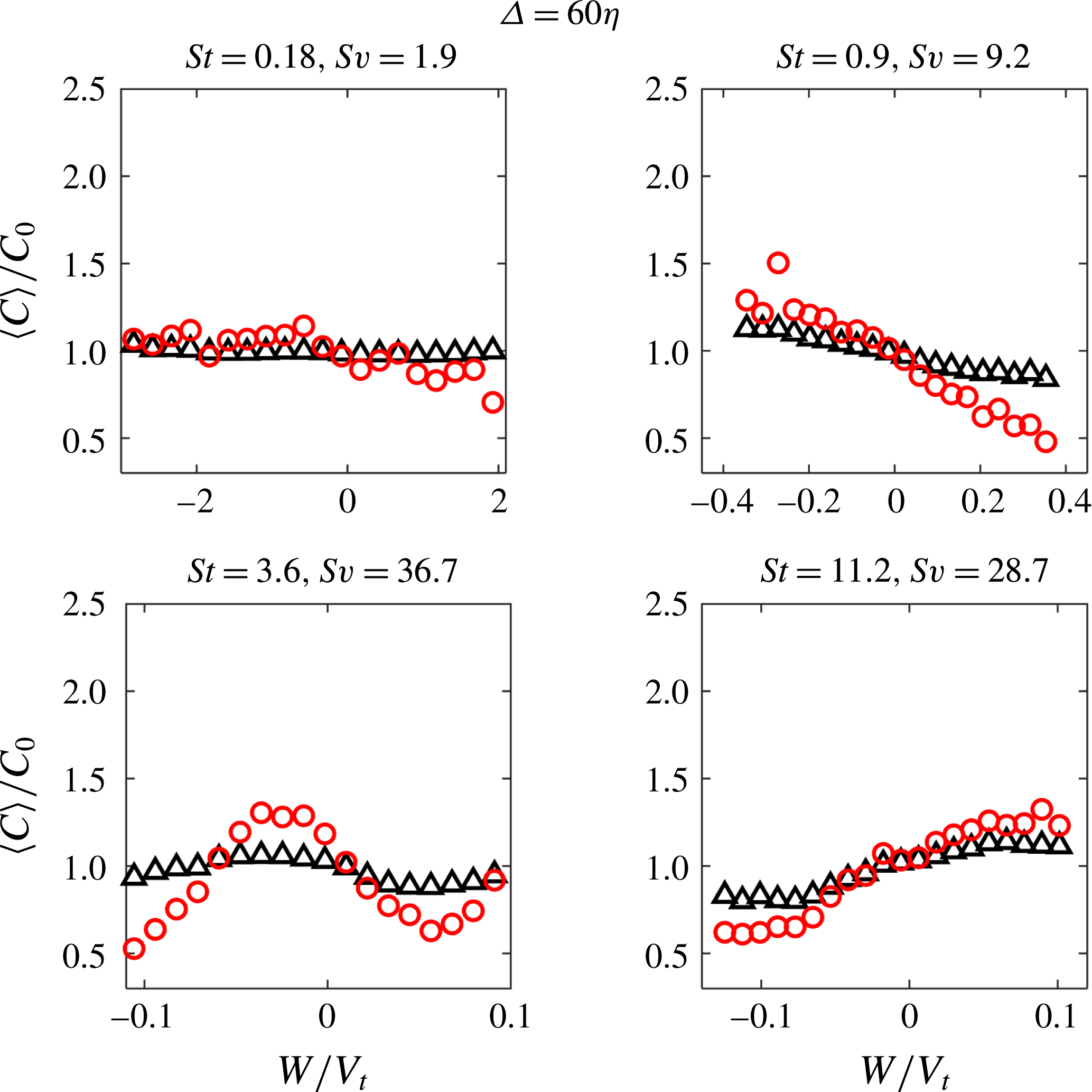
Local concentration for the settling P-I (black triangles) and P-IV particles (red circles), conditionally averaged on the normalized vertical fluid velocity using the low-pass-filtered velocity field.

Since we have shown that the coherent clusters of highly inertial particles sample high-strain low-vorticity regions in the low-pass-filtered velocity field, it is interesting to explore how they sample downward or upward regions of the filtered field. This is illustrated in figure 21, which is obtained from the velocity filtered at
 $\unicode[STIX]{x1D6E5}=60\unicode[STIX]{x1D702}$
. The clustered particles at
 $St=0.18$
,
 $Sv=1.9$
show much weaker preferential sweeping by the coarse-grained fluid velocity. The opposite is true for
 $St=0.9$
,
 $Sv=9.2$
particles, which appear to ‘resonate’ better with the filtered velocity field and clearly favour downward flow regions. The clustered particles at
 $St=3.6$
,
 $Sv=36.7$
exhibit a remarkable non-monotonic trend: for moderate vertical velocities they preferentially sample downward regions of the filtered field, while for strong vertical velocity they are rather found in upward regions. Finally,
 $St=11.2$
,
 $Sv=28.7$
particles clearly favour upward flow regions. Filtering at
 $\unicode[STIX]{x1D6E5}=30\unicode[STIX]{x1D702}$
returns the same qualitative picture. Taken together, these trends suggest that the effect of turbulence on the settling speed results from the combination of multiple mechanisms. The particles are centrifuged out of vortices with which they ‘resonate’ based on their response time (and as allowed by the time they can spend in the vortex vicinity, which is limited by the settling). Their fall speed is in this case enhanced (preferential sweeping). However the heavier particles cannot respond to the more intense and fast events, and they instead fall through these quick eddy motions, spending more time in the upward regions (loitering). Which mechanism prevails depends thus not only on the particle inertia, but also on the specific range of scales within the spectrum of the turbulent flow events. This behaviour is evidenced by particles belonging to coherent clusters much more so than by generic inertial particles.
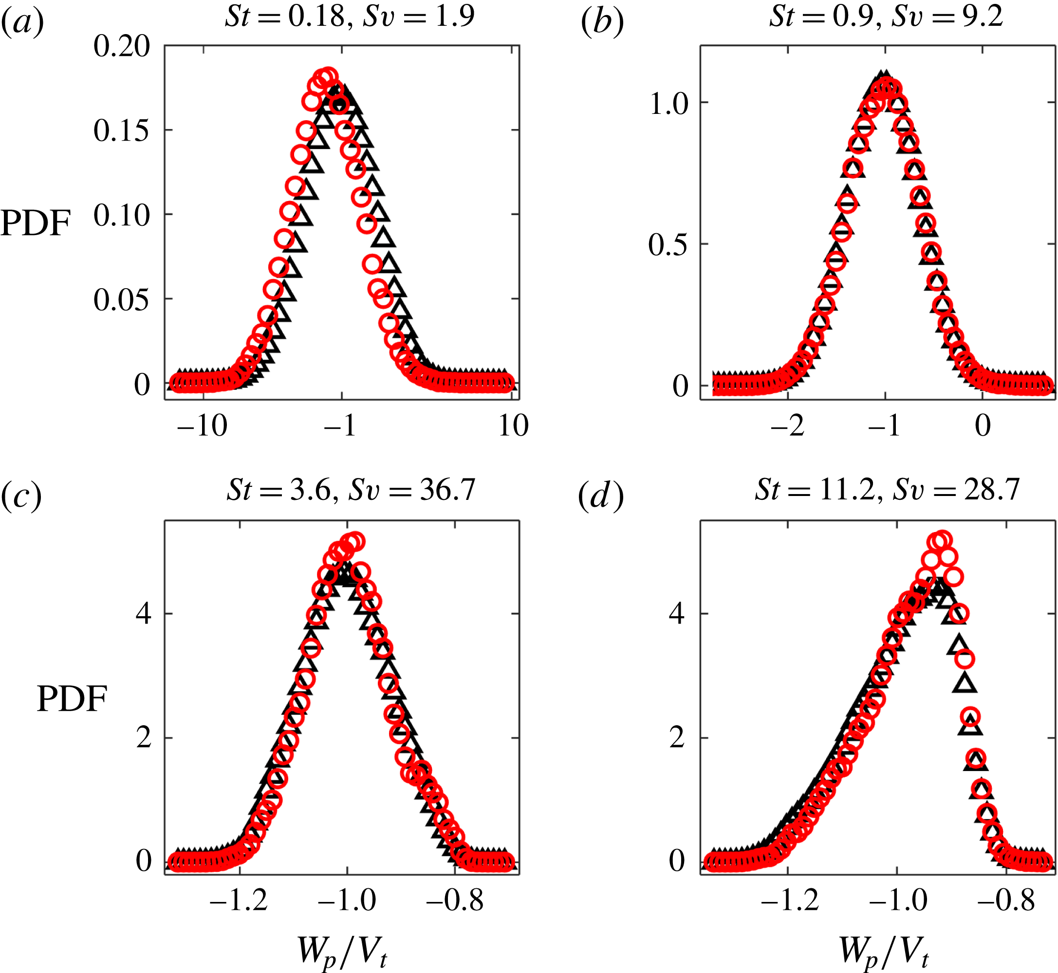
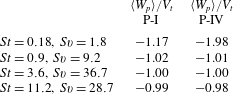
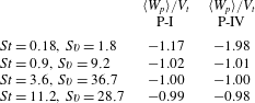
Figure 22 displays PDFs of normalized vertical velocity for P-I and P-IV particles, whose mean values are reported in table 5. Consistently with previous studies, a significant increase in settling velocity is found for St of order 1 and
 $Sv$
below 10 (Good et al.
Reference Good, Ireland, Bewley, Bodenschatz, Collins and Warhaft2014; Rosa et al.
Reference Rosa, Parishani, Ayala and Wang2016). For the
 $St=0.18$
,
 $Sv=1.9$
case the distribution is more positively skewed, and the settling velocity in the coherent clusters is more strongly enhanced compared to generic P-I particles. Indeed the mean settling velocity, which for the P-I particles is only 17 % higher than the theoretical still-fluid value
 $V_{t}$
, is almost twice as high as
 $V_{t}$
for the particles belonging to coherent clusters. Aliseda et al. (Reference Aliseda, Cartellier, Hainaux and Lasheras2002) also observed that inertial particles reached larger settling velocities when located in high-concentration regions, but given their volume fraction range they attributed this behaviour to the collective action of the clustered particles. In the present one-way coupled simulations no collective effect can ensue, therefore the large fall speed of the clusters must rather be a consequence of the more prominent preferential sweeping (figure 20).
PDFs of normalized vertical particle velocity for P-I (black triangles) and P-IV particles (red circles). The velocity range in the different cases has been adjusted to better represent the shape of the distributions.

Mean normalized vertical particle velocity for P-I and P-IV particles.
The settling velocity distributions at
 $St=0.9$
,
 $Sv=9.2$
and
 $St=3.6$
,
 $Sv=36.7$
are fairly symmetric, and the mean values are negligibly different from
 $V_{t}$
for both P-I and P-IV particles, confirming that for these St and
 $Sv$
levels the particles become uncorrelated from the flow structures that cause preferential sweeping. At
 $St=11.2$
,
 $Sv=28.7$
the mean settling velocity for the P-IV particles is 2 % smaller than
 $V_{t}$
. More evidently, the PDFs show strong negative skewness. This indicates that the particles are more likely to sample upward fluid motions which reduce their fall speed, but occasionally encounter downward sweeps, leading to intermittent and very rapid settling events. We interpreted this as further evidence of loitering, which typically acts on particles falling too quickly through the flow to react to the eddies and spend more time on average in upward-moving regions of the flow (Nielsen Reference Nielsen1993; Good et al.
Reference Good, Gerashchenko and Warhaft2012). In their DNS simulations, Good et al. (Reference Good, Ireland, Bewley, Bodenschatz, Collins and Warhaft2014) found that reduced settling only occurred when accounting for nonlinear drag. The present results suggest that this can in fact occur even when neglecting nonlinear drag (as done in the present simulations), but is only apparent when focusing on particles belonging to clusters.
Recent attempts have been made to further our understanding of particle–turbulence interaction under gravity effects, in particular by analysing the topology of the flow experienced by settling particles. Bec et al. (Reference Bec, Homann and Ray2014) provided an elegant analytical argument to show that, for
 $St\ll 1$
, the concentration of falling particles along horizontal planes is correlated with downward vertical fluid velocity, as already demonstrated numerically by Wang & Maxey (Reference Wang and Maxey1993) in homogeneous isotropic turbulence. They also showed that fast-falling particles with
 $St\geqslant 1$
experience more intense clustering as a consequence of an effectively two-dimensional dynamics along horizontal planes. Focusing on a similar range of parameters, Park & Lee (Reference Park and Lee2014) argued that fast-falling particles are more exposed to regions of converging fluid motion along horizontal planes, identified by negative in-plane divergence, i.e.
 $(\unicode[STIX]{x2202}U/\unicode[STIX]{x2202}x+\unicode[STIX]{x2202}U/\unicode[STIX]{x2202}y)=-\unicode[STIX]{x2202}W/\unicode[STIX]{x2202}z<0$
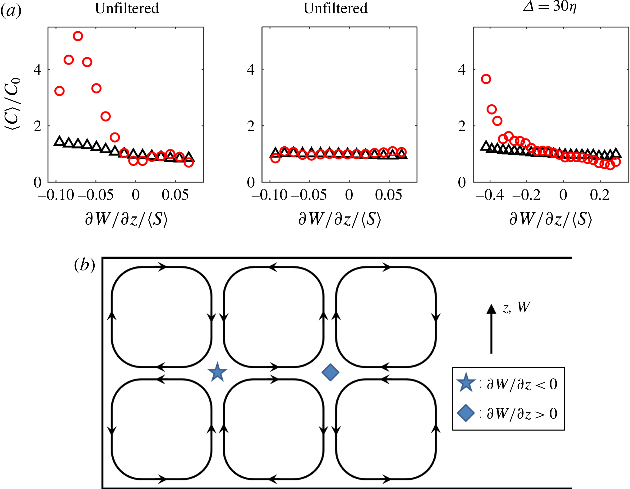
. In figure 23(a) we explore the correlation between particle concentration and the vertical strain rate
 $\unicode[STIX]{x2202}W/\unicode[STIX]{x2202}z$
(normalized by the mean strain rate
 $\langle S\rangle$
). For the
 $St=0.18$
,
 $Sv=1.9$
case, P-I particles show weak correlation with the in-plane divergence, while P-IV particles are more abundant in regions where
 $\unicode[STIX]{x2202}W/\unicode[STIX]{x2202}z<0$
, i.e. in regions of compressive vertical strain (i.e. positive horizontal-plane divergence). No significant correlation between concentration and
 $\unicode[STIX]{x2202}W/\unicode[STIX]{x2202}z$
is found for particles at
 $St=0.9$
,
 $Sv=9.2$
or higher (not shown). The correlation between concentration and compressive vertical strain contrasts the proposition of Park & Lee (Reference Park and Lee2014), but is indeed in agreement with the classic view of preferential sweeping. Considering a simple cellular flow (similar to the one studied first by Maxey & Corrsin (Reference Maxey and Corrsin1986) and Maxey (Reference Maxey1987), and recently revisited by Bergougnoux et al. (Reference Bergougnoux, Bouchet, Lopez and Guazzelli2014)), inertial particles that tend to favour the downward sweeps also tend to cluster in regions of
 $\unicode[STIX]{x2202}W/\unicode[STIX]{x2202}z<0$
, as illustrated in figure 23(b). While turbulent velocity fields are much more complex, the same qualitative picture for preferential sweeping was deduced by Wang & Maxey (Reference Wang and Maxey1993) by analysing DNS simulations. This behaviour is hardly visible when considering the totality of the inertial particles, but becomes apparent when considering the particles belonging to coherent clusters.
Local concentration of P-I (black triangles) and P-IV particles (red circles) conditioned on
 $\unicode[STIX]{x2202}W/\unicode[STIX]{x2202}z$
normalized by the global average of
 $S$
(a) for the
 $St=0.18$
,
 $Sv=1.9$
case with unfiltered velocity, the
 $St=0.9$
,
 $Sv=9.2$
case with unfiltered velocity, and the
 $St=0.9$
,
 $Sv=9.2$
case with low-pass-filtered velocity. The mechanism is illustrated in a sketch of a simple cellular flow (b), where inertial particles will tend to accumulate in regions of compressive vertical strain (marked with a star) rather than in regions of extensive vertical strain (marked with a diamond).

In figure 21 we have shown that clustered particles with
 $St=0.9$
,
 $Sv=9.2$
, which fall too fast to experience substantial preferential sweeping, still display a significant tendency to favour downward flow regions of a low-pass-filtered velocity field. In a similar manner, figure 23(a) shows that particles at
 $St=0.9$
,
 $Sv=9.2$
concentrate in regions where
 $\unicode[STIX]{x2202}W/\unicode[STIX]{x2202}z<0$
when the velocity field is low-pass-filtered at
 $\unicode[STIX]{x1D6E5}=30\unicode[STIX]{x1D702}$
. Once again, such effect is only visible when considering P-IV particles. Even heavier particles are uncorrelated with
 $\unicode[STIX]{x2202}W/\unicode[STIX]{x2202}z$
, independently of the filter size. Besides agreeing with the phenomenology of Maxey and co-workers, the correlation of the clustered particles with regions of compressive vertical strain may help explain the increase in cluster size with gravity for
 $St=0.18$
and
 $St=0.9$
(see table 4), as it could provide a mechanism for the particles to ‘pile up’ as they fall through these flow regions. It does not, however, explain the larger and vertically elongated clusters generated at
 $St=3.6$
and
 $St=11.2$
, since in these cases no significant correlation with
 $\unicode[STIX]{x2202}W/\unicode[STIX]{x2202}z$
is found. The cluster size and orientation in presence of gravity is further discussed in the next section.
4.6 Cluster orientation
The identification of coherent clusters allows an investigation of their individual spatial orientation. In particular, to determine the effect of gravity on their orientation, we calculate the angle
 $\unicode[STIX]{x1D703}_{g}$
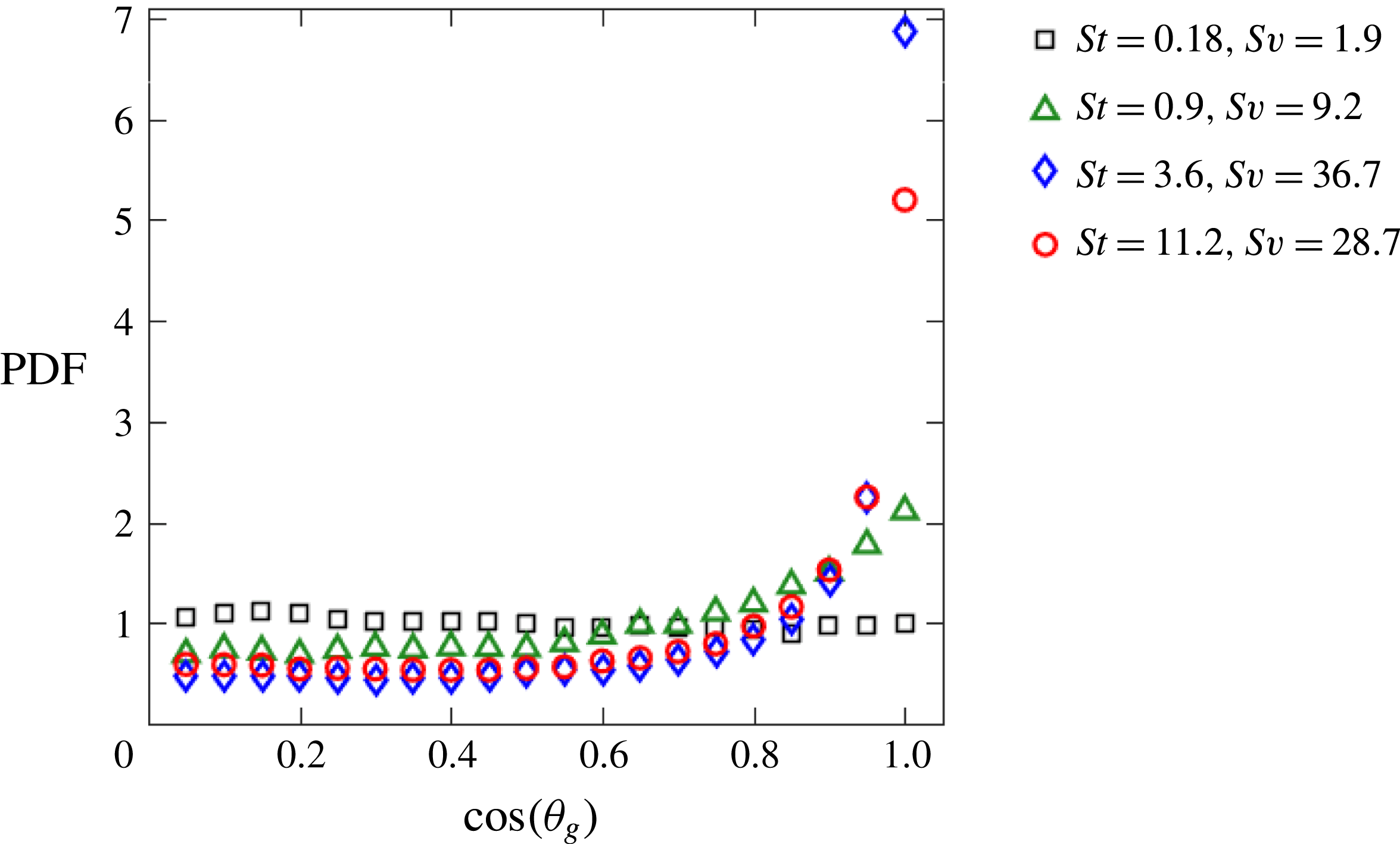
between the vertical axis and the primary cluster axis determined by the SVD method. The PDF of the cosine of
 $\unicode[STIX]{x1D703}_{g}$
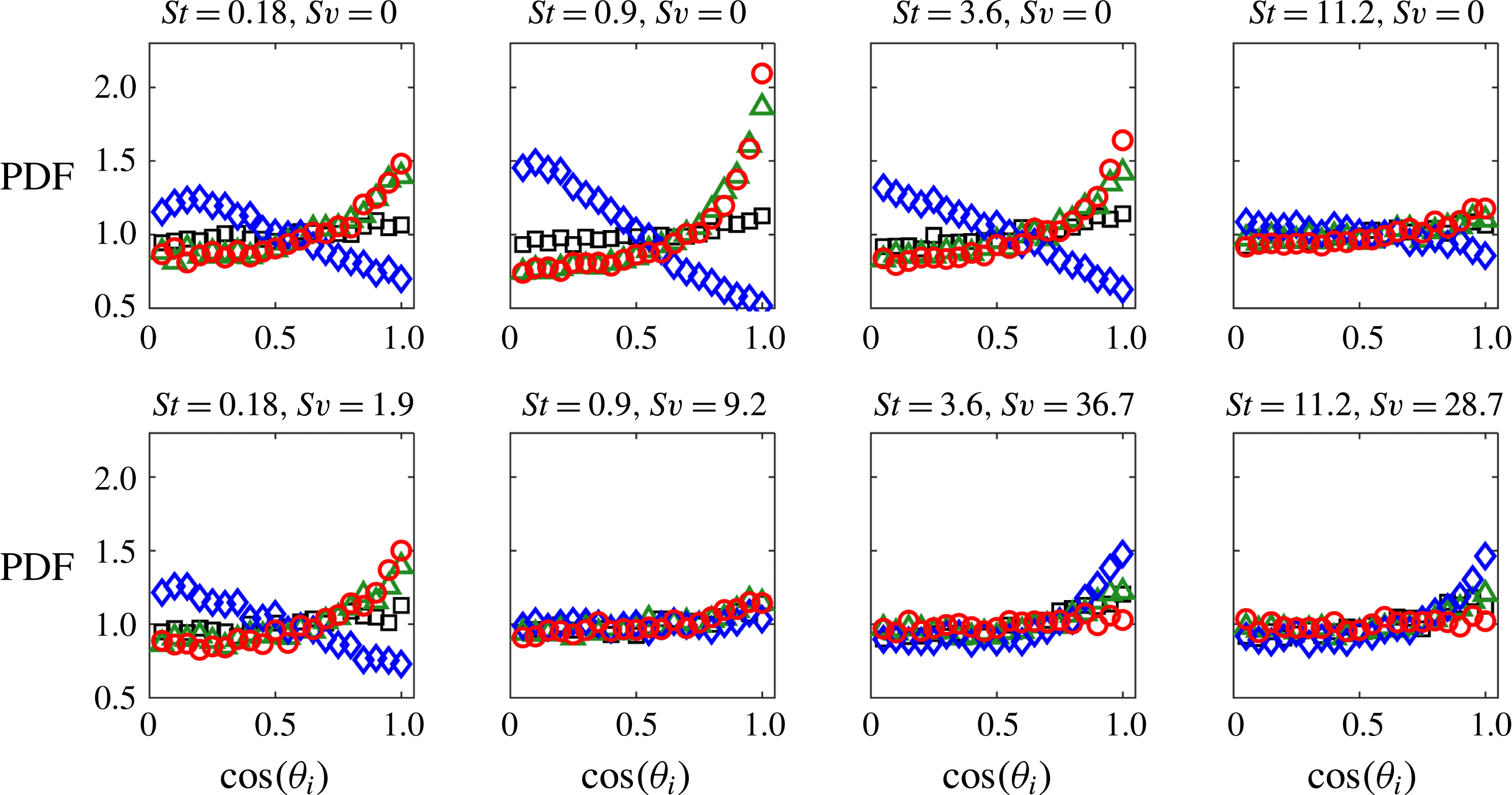
is shown in figure 24 for each case. Heavier particles have a stronger tendency to form vertically oriented clusters, in agreement with the visual evidence that fast-falling particles form long, vertical streaks (figure 5) and with the ADF analysis (figure 13). As expected, the degree of this effect appears to be determined by
 $Sv$
rather than by St.
PDFs of the cosine of cluster orientation angle
 $\unicode[STIX]{x1D703}_{g}$
for coherent clusters.

The presence of large, vertically elongated clusters of heavy, fast-falling particles has been noted in several previous studies also focused on one-way coupled point-particle simulations (Woittiez et al.
Reference Woittiez, Jonker and Portela2009; Dejoan & Monchaux Reference Dejoan and Monchaux2013; Bec et al.
Reference Bec, Homann and Ray2014; Park & Lee Reference Park and Lee2014; Ireland et al.
Reference Ireland, Bragg and Collins2016). Clearly, given the nature of the modelling approach, this behaviour cannot be explained by long-range multi-particle hydrodynamic interactions, as in columnar settling of suspensions of particles at relatively large Reynolds numbers (e.g. Uhlmann & Doychev Reference Uhlmann and Doychev2014). Previously the vertical alignment of the clusters has been related to a two-dimensionalization of the dynamics in the horizontal plane (Bec et al.
Reference Bec, Homann and Ray2014; Park & Lee Reference Park and Lee2014), and to the influence of settling on the balance between inward drift and outward diffusion of particle pairs (Ireland et al.
Reference Ireland, Bragg and Collins2016). However, a conclusive explanation has not yet emerged, especially to justify the large extension of these structures. The skewed distribution of vertical velocities for the
 $St=11.2$
,
 $Sv=28.7$
case in figure 22(d) suggests an alternative mechanism for the formation of the vertically elongated clusters: while high-St particles spend more time in upward-moving fluid regions (hence experiencing loitering), they sometimes encounter a strong downward gust of turbulence which, adding to their already high fall speed, projects them ballistically through the flow. These correspond to the extreme events of highly negative velocity that make up the left tail of the PDF in figure 22(d). For the duration of such gust, all particles that pass through the corresponding flow region are channelled vertically downward, creating columnar structures. This reasoning can also be used to explain the vertically elongated clusters at lower Stokes number, although it is more effective for more inertial particles. The mechanism would cease to play a role for particles so heavy as to be completely unaffected by the flow, which would remain randomly distributed. While this view (which shares conceptual similarities with the path-history effects discussed in Bragg & Collins (Reference Bragg and Collins2014) and Ireland et al. (Reference Ireland, Bragg and Collins2016)) is consistent with the observations, it awaits to be confirmed by dedicated investigations on the cluster formation and evolution.
PDFs of the cosine of the angles
 $\unicode[STIX]{x1D703}_{i}$
between the cluster primary axis and the cluster-averaged vectors
 $\boldsymbol{e}_{1}$
(black squares),
 $\boldsymbol{e}_{2}$
(green triangles),
 $\boldsymbol{e}_{3}$
(blue diamonds), and
 $\unicode[STIX]{x1D6FA}$
(red circles) for coherent clusters.

In order to determine how cluster orientation is affected by the local velocity field, we calculate the angle
 $\unicode[STIX]{x1D703}_{i}$
between the primary axis of each coherent cluster and four vectors describing the local flow topology: the extensive, intermediate, and compressive eigenvectors of the strain-rate tensor (
 $\boldsymbol{e}_{1}$
,
 $\boldsymbol{e}_{2}$
, and
 $\boldsymbol{e}_{3}$
, respectively), and the local vorticity vector,
 $\unicode[STIX]{x1D6FA}$
. For each cluster, these quantities are obtained from the average over the grid points contained within the volume of each cluster. The PDFs of the cosine of the four angles are shown in figure 25. For zero or moderate
 $Sv$
, the clusters tend to be strongly aligned with the local vorticity vector. It is well known that the vorticity tends to be indifferently aligned with
 $\boldsymbol{e}_{1}$
, strongly aligned with
 $\boldsymbol{e}_{2}$
, and strongly anti-aligned with
 $\boldsymbol{e}_{3}$
(Ashurst et al.
Reference Ashurst, Kerstein, Kerr and Gibson1987; Vincent & Meneguzzi Reference Vincent and Meneguzzi1991; Tsinober, Kit & Dracos Reference Tsinober, Kit and Dracos1992; Hamlington, Schumacher & Dahm Reference Hamlington, Schumacher and Dahm2008; Buxton & Ganapathisubramani Reference Buxton and Ganapathisubramani2010). The PDFs show that the clusters follow the same alignment with the strain-rate eigenvectors as the vorticity vector, confirming that the alignment with the latter is an inherent feature of coherent clusters. This result is consistent with (but not implied by) the classic picture of the particles being centrifuged outside of vortex cores and collecting around vortices (Eaton & Fessler Reference Eaton and Fessler1994; Calzavarini et al.
Reference Calzavarini, Kerscher, Lohse and Toschi2008). Moreover, Ni, Ouellette & Voth (Reference Ni, Ouellette and Voth2014) recently showed that the vorticity vector tends to align with the direction of maximum Lagrangian stretching. It is therefore possible that, over times comparable with the clusters’ lifetime, groups of particles with St of order unity (and marginally or moderately affected by gravity) become elongated as they are carried by the fluid that undergoes vortex stretching, and therefore end up forming a cluster aligned with the vorticity vector. To confirm this proposition, a detailed investigation of the Lagrangian cluster properties is required, which is beyond the scope of the present study.
Another observation prompted by figure 25 is that the high-
 $Sv$
clusters, while showing no preferential alignment with the vorticity vector, have a noteworthy tendency to align with the compressive strain-rate eigenvector,
 $\boldsymbol{e}_{3}$
. The dynamics behind this result are not clear and deserve further investigation.
5 Conclusions and discussion
We have introduced a definition of inertial particle clusters that takes into account not only the local concentration, but also the self-similar nature of the underlying turbulence. Beyond constraints on concentration and connectivity, clusters are considered dynamically relevant if they are large enough to exhibit self-similarity, as deduced from their size distribution and the fractal nature of their delimiting surface area. The proposed cluster identification approach leverages the Voronoï diagram method, but is also compatible with other tessellation techniques.
In order to explore the properties of these coherent clusters, we have used one-way coupled simulations of particle-laden homogeneous isotropic turbulence, with physical parameters relevant to dispersions of liquid or solid particles in gas flow. The study is not meant to provide a comprehensive description of cluster behaviour as a function of flow and particle properties. Rather, it gives a sample of the several properties that can be defined and investigated following the identification of clusters as individual objects. We have therefore focused on a number of selected cases that highlight important particle–turbulence dynamics. The cluster analysis brings significant new insight into well-known mechanisms such as preferential concentration and modification of settling rate by turbulence. In addition, it provides novel information on the topology and behaviour of particle clusters. The particles that belong to them are only a small fraction (typically a few percent) of the total. However, we remark that this is not due to the fact that we restrict our attention to self-similar clusters (group P-IV). Rather, the greatest reduction in particle number is due to considering connected sets of particles having volume cells
 $V<V^{\ast }$
(group P-III). Such a definition of clusters was used by most previous studies which identified individual clusters (e.g. Monchaux et al.
Reference Monchaux, Bourgoin and Cartellier2010; Zamansky et al.
Reference Zamansky, Coletti, Massot and Mani2016; Sumbekova et al.
Reference Sumbekova, Cartellier, Aliseda and Bourgoin2017). Moreover, although they make up a limited fraction of all particles, the coherently clustered particles are in high concentration over extended regions of space (notably, larger than the viscous scales of the flow), and therefore we expect them to play an important role in the multiphase dynamics – for example, in their back-reaction on the flow by exchange of momentum and/or heat. Some of these dynamics were recently demonstrated in Frankel et al. (Reference Frankel, Pouransari, Coletti and Mani2016) and Zamansky et al. (Reference Zamansky, Coletti, Massot and Mani2016).
At the considered
 $Re_{\unicode[STIX]{x1D706}}$
, the volume threshold for geometric self-similarity is found to be
 $8\unicode[STIX]{x1D702}^{3}$
for a wide range of St and
 $Sv$
. The size of the identified clusters span from the viscous to the integral scales, with average concentrations that depend on St and
 $Sv$
, but not on the cluster volume. The particles associated to coherent clusters exhibit a significantly higher degree of spatial organization and local accumulation, as measured by their RDFs. The structure of the clusters is characterized through various fractal dimensions. The correlation dimension follows similar trends with St and
 $Sv$
as for the whole particle field, while the box-counting dimension has similar values as in previous studies for high-shear turbulent structures. The surfaces delimiting the clusters have fractal dimensions of 2.85 or larger for all considered cases, underscoring their highly convoluted, space-filling geometry. Therefore the definition of cluster shape, and in particular aspect ratio, is not straightforward and depends on the technique used to calculate it. On average, the clusters do appear as elongated objects, but with increasing size they seem to transition from tubular to planar to globular. Under the effect of gravity-elongated shapes prevail, with a strong tendency to align with the vertical direction.
Compared to the general inertial particles, those belonging to coherent clusters display a much stronger tendency to sample high-strain, low-vorticity regions (preferential concentration). Even for St significantly larger than unity, such tendency is still visible if one considers a velocity field low-pass-filtered at scales comparable to the integral length of the turbulence. This is consistent with both the classic picture of particles being centrifuged by turbulent eddies, and with the more recent view that clustering happens over a range of scales depending on the Stokes number.
Recently, other mechanisms different from the eddy centrifuging effect have been proposed to explain the appearance of particle clusters. In particular, Vassilicos and collaborators observed that inertial particles tend to stick to the zero-acceleration points of the flow (a behaviour they termed sweep-stick mechanism), which in turn organize themselves in multi-scale clusters (Chen, Goto & Vassilicos Reference Chen, Goto and Vassilicos2006; Goto & Vassilicos Reference Goto and Vassilicos2008). While the centrifuging mechanism seems to provide a natural justification for the small-scale clustering of low-St particles in flows with relatively low Reynolds numbers, it has been argued that the sweep-stick mechanism better explains the multi-scale clustering at higher Reynolds numbers, which occurs also for particles with stopping times comparable to the inertial scales (Yoshimoto & Goto Reference Yoshimoto and Goto2007; Coleman & Vassilicos Reference Coleman and Vassilicos2009). Recent experimental studies have brought support to the sweep-stick mechanism by showing that clustered particles reflect better the topology of zero-acceleration points than the one of low-vorticity points (Obligado et al.
Reference Obligado, Teitelbaum, Cartellier, Mininni and Bourgoin2014). The present results confirm that not only the particle concentration field as a whole, but also the individual clusters display a strongly multi-scale behaviour. However, we also show that individual coherent clusters of particles with relatively large St still oversample high-strain/low-vorticity regions of the flow, if one considers only the large-scale structures (which we have done here by low-pass-filtering the velocity field). Coleman & Vassilicos (Reference Coleman and Vassilicos2009) applied a similar approach to the entire particle field and found instead that particles with
 $St_{\unicode[STIX]{x1D702}}>1$
did not oversample high-strain regions of the low-pass-filtered turbulent field. A possible interpretation is that, even at relatively high Stokes number, the centrifuging mechanism is able to produce individual clusters, which however account for a relatively small fraction of all particles. The results, however, may also be consistent with a more comprehensive view in which the centrifuging mechanism prevails at low Stokes numbers, while the sweep-stick mechanism prevails for particles with response times in the inertial range (Coleman & Vassilicos Reference Coleman and Vassilicos2009). We point out that our investigation considers a relatively modest turbulent Reynolds number, and therefore one should not draw definitive conclusions on a matter in which scale separation plays a significant role. For example, the sweep-stick mechanism suggests that the particle Stokes number should not majorly affect the clustering properties as long as the particle response time is much smaller than the integral time scale of the flow; a view that recently found support in the measurements of Sumbekova et al. (Reference Sumbekova, Cartellier, Aliseda and Bourgoin2017). Our simulations show a strong dependence of the cluster volume with Stokes number, but this could be due to the low Reynolds number, which makes the constraint on the particle response time quite stringent (see the discussion in Sumbekova et al.
Reference Sumbekova, Cartellier, Aliseda and Bourgoin2017).
When gravity is acting, particles inside coherent clusters with
 $Sv$
of order unity strongly oversample downward flow regions (preferential sweeping). In the present turbulence conditions this leads to a mean settling velocity nearly doubled with respect to still-fluid terminal velocity. In comparison, the settling velocity averaged over all particles is only increased by 17 %. In this regime particle clustering correlates well with regions of compressive vertical strain, i.e. regions of positive two-dimensional divergence along horizontal planes. If low-pass-filtered velocities are considered, preferential sweeping is visible for particles in coherent clusters with
 $Sv$
up to around 10. At even higher
 $Sv$
, the most inertial particles in coherent clusters exhibit markedly skewed vertical velocity distributions, and favour regions of upward flow, which slightly reduces their mean settling velocity (loitering). In the present simulations, this is not the consequence of nonlinear drag, which we have neglected. The skewed settling velocity distribution of the heavier particles suggests that, while they spend more time in upward-moving fluid regions, occasional gusts of downward flow may cause them to bullet through the fluid. We have argued that this interaction may explain the appearance of columnar particle clusters in the present one-way coupled simulations. Clustering is found to be stronger in the presence of gravitational settling; this seems at odds with the centrifuging mechanism, since settling is expected to de-correlate the particles from the turbulent structures. Ireland et al. (Reference Ireland, Bragg and Collins2016) argued that, for
 $St>1$
, such behaviour can be explained considering the path-history effect (Bragg & Collins Reference Bragg and Collins2014): inertial particles retain memory of the different fluid fluctuations they have experienced, and therefore may have high relative velocities, a mechanism which reduces clustering for high-St particles; because gravitational settling hinders this path-history effect, clustering is overall enhanced. As mentioned, the sweep-stick mechanism is also a candidate to explain inertial-range clustering of high-St particles, although the mechanism has not been explored in cases in which settling is important.
One of the major findings of the present study is that clusters of preferentially concentrated particles have a strong tendency to align with the local vorticity vector. Because the latter is in turn aligned with the direction of maximum Lagrangian stretching, this provides hints on the cluster formation process, which could be seen as sets of particles being elongated during vortex stretching. This and other interesting points related to the formation and lifetime of the clusters can be addressed by using the proposed cluster definition in concert with a Lagrangian analysis of time-varying quantities. In particular, in order to reach a univocal definition of coherent clusters, their temporal coherence shall also be assessed. Further research in this area is warranted.
The limitations of the present computational approach need to be kept in mind when interpreting the results. Our one-way coupled point-particle simulations ignore the particle mass loading effects and particle–particle interaction, which can play a significant role when the concentration is increased by clustering. While the average in-cluster concentration is only one order of magnitude higher than the domain average, the RDFs at small separations and the PDF of Voronoï cell volumes indicate that local peaks can be much higher. Therefore, our results, especially at small scales, should be interpreted with caution and await verification by experiments and fully resolved simulations.
The proposed analysis can be readily applied to existing simulations, and may be particularly fruitful to mine recent data at high
 $Re_{\unicode[STIX]{x1D706}}$
(e.g. Calzavarini et al.
Reference Calzavarini, Kerscher, Lohse and Toschi2008; Ireland et al.
Reference Ireland, Bragg and Collins2016; Rosa et al.
Reference Rosa, Parishani, Ayala and Wang2016), whose wide scale separation would provide further insight into the self-similar cluster structure. Finally, the study of coherent clusters is expected to be especially relevant to the two-way and four-way coupled regimes, where the properties of sets of highly concentrated particles are of paramount importance for the inter-phase transfer of momentum and energy. In particular, since self-similar clustering occurs already at dissipative scales, over which it has been shown that extremely high concentrations can occur, particle loading and collision effects may potentially play a strong role in the formation, evolution, and behaviour of individual clusters.
Acknowledgements
This work was supported by the United States Department of Energy under the Predictive Science Academic Alliance Program 2 (PSAAP2) at Stanford University. The authors acknowledge the Minnesota Supercomputing Institute (MSI) at the University of Minnesota for providing computational resources that contributed to the results reported within this paper, and in particular E. Bollig for his help in developing the cluster detection algorithm. We have benefited from stimulating discussions with G. Voth and A. Banko.